Impact of three intense winter cyclones on the sea ice cover in the Barents Sea: A case study with a coupled regional climate model

1 Introduction

In winter, the North Atlantic storm track has a large influence on the climate conditions in the Atlantic sector of the Arctic Ocean. Particularly the interannual variability of the Barents-Kara Sea (BKS) sea ice in winter is primarily driven by atmospheric processes (Liu et al., 2022). Mechanisms include changes in the atmospheric circulation patterns, wind field, and longwave downward radiation (LWD), e.g., due to inflow of warm-moist air (Park et al., 2015; Woods and Caballero, 2016; Zhang et al., 2023). Synoptic cyclones play an important role here (Sorteberg and Kvingedal, 2006; Rinke et al., 2017; Graham et al., 2019) and exert significant impacts on sea ice concentration (SIC) (Kriegsmann and Brümmer, 2014; Schreiber and Serreze, 2020; Valkonen et al., 2021; Aue et al., 2022; Clancy et al., 2022) and sea ice thickness (SIT) (Boisvert et al., 2016; Ricker et al., 2017a) in winter. Generally, the impacts on sea ice are related to both dynamic and thermodynamic atmospheric forcing. For the former, strong surface winds and rapid changes in wind direction related to cyclone passages can trigger divergent/convergent sea ice motion with impact on SIC through opening/closing of leads and on SIT through ice compression and possible formation of pressure ridges as well as through enhanced ice growth in case of increasing lead fraction (Itkin et al., 2017). Thermodynamically, the advection of warm-moist/cold-dry air at the cyclones front/back side favors positive/negative anomalies in LWD and sensible heat fluxes. The resulting reduced/increased energy loss at the surface finally leads to lower/higher sea ice growth rates (SGR) in winter (Cai et al., 2020).

The understanding of these mechanisms is important for sea ice forecasts (Serreze and Stroeve, 2015; Wayand et al., 2019), particularly during hazardous weather systems such as storms, typically associated with strong cyclones. Such conditions are challenging for Arctic navigation (Inoue, 2021), aviation (Gultepe et al., 2019), and other human activities. Furthermore, understanding of the mechanisms helps to improve weather and climate models with respect to the simulations of storm interactions with the underlying ocean, including sea ice. This is important for a better understanding of how cyclone impacts might evolve under diminishing and thinner sea ice conditions in the future (Cai et al., 2020). Considering the accelerated winter sea ice retreat in BKS (Liu et al., 2022), such research is of primary importance.

Over the last decades, a decrease in sea ice extent and thickness has been observed over the Arctic Ocean (e.g., Kwok, 2018; Meier and Stroeve, 2022). Particularly a thinning of the sea ice cover is relevant for its response to cyclones, because thinner ice is more sensitive to atmospheric forcing. Evidence for this is given by an observed increase in ice deformation and drift speed under thinner ice conditions (e.g., Rampal et al., 2009; Spreen et al., 2011). There is also indication that thinner sea ice is more vulnerable to break-up events under strong winds (Rheinlaender et al., 2022), which are often associated with cyclone passages. Additionally, cyclones can have stronger thermodynamic impacts on a thinner ice cover, because thinner ice grows faster than thicker ice (e.g., Haas, 2017; Petty et al., 2018).

However, the relative contributions of the dynamic and thermodynamic processes to the cyclones’ impacts on winter sea ice are still not well known. The few existing studies arrive at mixed results. Based on an analysis of daily SGR under the impact of winter cyclones in the Nordic Seas in CMIP5 models, Cai et al. (2020) found that the absolute value of the thermodynamic SGR change exceeds the dynamic contribution in response to strong cyclonic circulation. In observation-based studies, Schreiber and Serreze. (2020) came to the same conclusion for SIC response to cyclones, while Clancy et al. (2022) argued that both processes are important and comparable in magnitude. Further, Clancy et al. (2022) stressed that dynamic processes are the primary reason for the front/back side difference in the sea ice response to cyclones and particularly dominate the response of SIT to cyclones. The dominance of dynamics with respect to SIT changes is supported by a recent case study of the record Arctic cyclone in January 2022 by Blanchard-Wrigglesworth et al. (2022). Apart from that, Cai et al. (2020) found that the dynamic and thermodynamic responses of SGR to strong cyclones have a similar spatial pattern across different models, but there is no clear agreement on the sign. One model simulates anomalies of dynamic and thermodynamic SGRs with same sign, while the dynamic and thermodynamic SGRs offset each other in two other models. For Arctic moisture intrusion events, Park et al. (2015) showed that the LWD-related thermodynamic processes are dominant (and last as long as 1–2 weeks) for sea ice reductions after the first couple of days, which are characterised mostly by sea ice changes due to dynamics.

More generally, Koo et al. (2021) discussed that dynamic contributions may account for about 35% of the total increase of the mean SIT during the ice-growing season in the central Arctic Ocean. Moreover, von Albedyll et al. (2022) emphasized a possible large dynamic thickening via rafting and ridging under conditions of mobile, unconsolidated sea ice pack. However, the inclusion of SIT in the analysis of cyclone-related sea ice changes is challenging. It is reasonable to assume that a smaller SIT promotes stronger cyclone impacts because a thinner sea ice is more susceptible to atmospheric and oceanic forcings (Zhang et al., 2012; Rheinlaender et al., 2022). Limited daily SIT data hamper a systematic analysis and thus the few results rely on case studies and/or modeling (Boisvert et al., 2016; Cai et al., 2020). In conclusion, the relative importance of dynamic and thermodynamic mechanisms for cyclone impacts on the sea ice cover in winter remains a topic of research interest.

The objective of this study is to quantify the dynamic and thermodynamic contributions to changes in SIC and SIT in response to a sequence of cyclones in the BKS in winter and to explore the related mechanisms in detail, utilizing a coupled regional climate model. The presented sequence of cyclones consists of three intense storms that passed through the BKS in mid-February 2020. Using these cyclone cases as an example, we evaluate the spatial patterns of cyclone-induced sea ice changes in winter and discuss their dependencies on the state of the sea ice cover. An additional objective is to determine whether the sea ice has a memory of preceding cyclone passages that might influence its response to cyclones that follow.

2 Data and methods

2.1 HIRHAM–NAOSIM simulation

In our analysis of cyclone impacts on the Arctic sea ice cover we rely on a coupled model simulation, which enables us to decompose the sea ice changes into dynamic and thermodynamic contributions. The simulation was performed applying version 2.2 of the coupled regional climate model HIRHAM–NAOSIM. This version represents a further development of the base version 2.0, which is described and evaluated by Dorn et al. (2019). Version 2.2 includes new parameterizations and changed parameter settings. The differences between the two versions are listed in the Supplementary Material.

HIRHAM–NAOSIM is applied over a circum-Arctic domain using rotated latitude-longitude grids with horizontal resolution of 1/4° (∼ 27 km) in the atmosphere component HIRHAM and 1/12° (∼ 9 km) in the ocean–sea ice component NAOSIM. More detailed information on the model components and their coupling are given by Dorn et al. (2019).

The simulation was initialized on 1st of January 2019 and run through 31st of December 2020, driven by ERA5 reanalysis data (Hersbach et al., 2020) at HIRHAM’s lateral boundaries as well as HIRHAM’s lower and NAOSIM’s upper boundaries, which lie outside the coupling domain (defined as the overlap area of the components’ model domains). For NAOSIM’s open lateral boundaries, ORAS5 reanalysis data (Zuo et al., 2019) were used. HIRHAM was initialized with the corresponding ERA5 fields, while NAOSIM was started from rest with temperature, salinity, ice thickness, and ice concentration fields from ORAS5. HIRHAM’s prognostic fields were nudged to the corresponding ERA5 fields with a uniform nudging time scale of 16.67 h (which corresponds to a nudging of 1% per time step).

2.2 Supplementary evaluation data

We complement the HIRHAM–NAOSIM simulation with in-situ observations obtained during the Multidisciplinary drifting Observatory for the Study of Arctic Climate (MOSAiC) expedition (Shupe et al., 2020) and ERA5 reanalysis data to demonstrate that the model is able to 1) capture the synoptic situation (Supplementary Figures S1, S2) and 2) produce a realistic spatial pattern of SIC changes (Supplementary Figure S3) during the cyclone passages. It should be noted that the ERA5 SIC field is highly smoothed and has limitations to represent the observed strong gradient in SIC across the MIZ (Renfrew et al., 2021). However, for this cyclone case, the spatial patterns of SIC changes based on ERA5 are in strong agreement with high-resolution satellite derived SIC data based on AMSR (not shown). To further evaluate the simulated sea ice thickness (SIT) with remote sensing observations (Supplementary Figure S4), we utilize merged CryoSat-2 and SMOS satellite data (Ricker et al., 2017b).

During February 2020, RV Polarstern was located close to the North Pole in the central Arctic (Figure 1). The supplementary model evaluation is based on data from the 10-m meteorological flux tower installed at the meteorological observatory (Met-City) (Cox et al., 2021a) located in approximately 500 m distance to the RV Polarstern, three autonomous Atmospheric Surface Flux Stations (ASFS) (Cox et al., 2021b; Cox et al., 2021c) situated in the Distributed Network in a distance of approximately 25 km to RV Polarstern (Shupe et al., 2022), and a microwave radiometer HATPRO (Humidity and Temperature Profiler) (Walbröl et al., 2022). We use data averaged to 3-hourly resolution of 2-m air temperature, vertically integrated water vapour (IWV; 0–10 km height), mean sea level pressure (SLP) and 10-m wind speed. For the comparisons with the simulation, we use the nearest model grid-cell. IWV in the model simulation is the integrated specific humidity over all vertical levels from the surface up to the top (10 hPa, approx. 35 km height). To further evaluate the simulated spatial patterns of meteorological variables, we use 3-hourly ERA5 gridded data of 2-m air temperature, IWV, and SLP. We also use daily SIC data from ERA5, which are based on satellite data (HadISST2 and OSI SAF; see Hersbach et al., 2020).

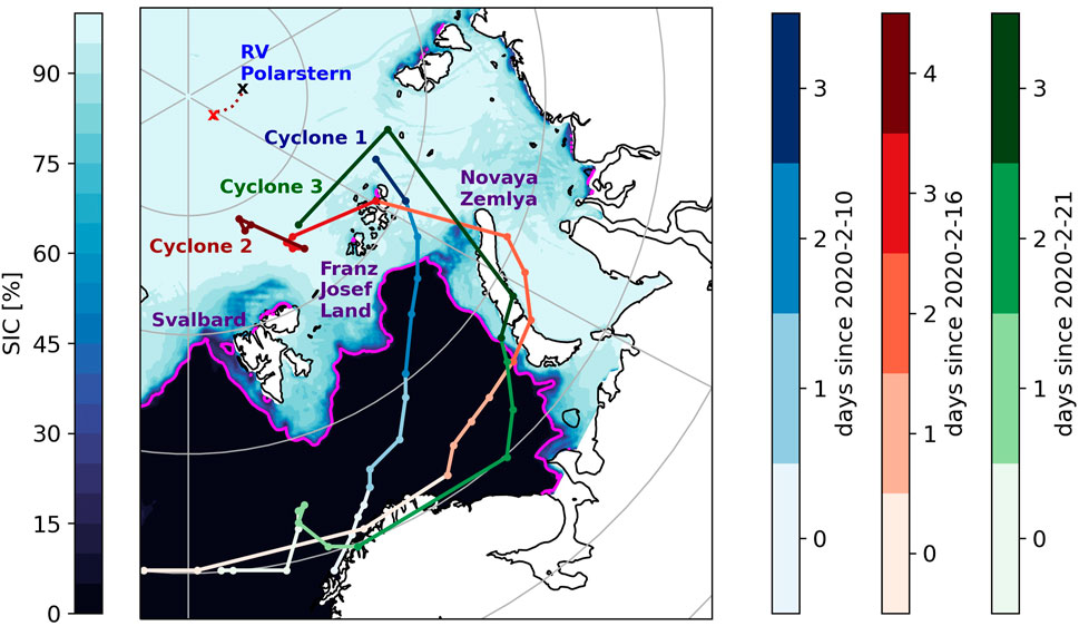
FIGURE 1. Track of cyclones 1, 2, and 3 (based on 6-hourly SLP minima in the study domain), indicated as blue, orange, and green lines, where the line color changes from bright to dark from the start to the end of the respective track. The position of the RV Polarstern at the start of the first (end of the third) cyclone event is marked as black (red) cross. Daily mean SIC and the 15% SIC contour (pink line) are shown for the day before the start of the first of the three cyclone passages (9 February 2020). SIC and cyclone tracks are based on the HIRHAM–NAOSIM simulation.

2.3 Dynamic and thermodynamic contributions to sea ice changes

The main objective of this study is to separately quantify dynamic and thermodynamic sea ice changes during and after the cyclone passages to gain insights into the underlying mechanisms. We approach this by temporally integrating HIRHAM–NAOSIM’s dynamic and thermodynamic SIT and SIC tendencies for specific time periods in order to decompose the overall sea ice changes in its respective components.

The overall sea ice changes are given by the model’s continuity equations for SIT (h) and SIC (A) as

where $\vec{v}$ is the ice velocity and $S_h^{\text{ice}}$, $S_h^{\text{ow}}$, $S_A^{\text{ice}}$, and $S_A^{\text{ow}}$ are the thermodynamic growth rates, which are separately calculated for the ice-covered (superscript ‘ice’) and the open water part (superscript ‘ow’) of the grid cell. A detailed description of the thermodynamic growth rates is given by Dorn et al. (2009). The term D_A represents the formation rate of open water due to shearing deformation (ridging) and is given as

where Δ represents the total deformation, determined by the strain rate tensor ${\dot{ϵ}}_{ij}$ (see Hibler, 1979), and K = 20 is an empirical constant. Consequently, the dynamic SIT and SIC tendencies are defined as

and the thermodynamic SIT and SIC tendencies are

Generally, we analyze these sea ice tendencies in concert with simulated changes in sea ice drift and surface energy budget (SEB). Since we focus on the impact of atmospheric variability on the sea ice–ocean system, we define the SEB as the sum of atmospheric net radiative, sensible, and latent heat fluxes at the surface, with positive values corresponding to a surface energy gain. To cover the importance of the ocean for (thermodynamic) sea ice processes, we additionally provide information on upward oceanic heat fluxes when discussing thermodynamic sea ice changes in Section 3.3.1.

3 Results

3.1 Cyclone cases

From February 9 to 25, 2020, a sequence of three cyclones travelled through the BKS (Figure 1), shaped the local weather conditions, and led to shifts in the position of the sea ice edge (15% SIC contour). The minimum SLP in the core of the cyclones was below 970 hPa (when crossing the sea ice edge) for all events, which is an extremely low value compared to climatological SLP conditions in the BKS region. Consequently, all three events can be classified as intense, stronger than normal cyclones (following Rinke et al., 2017). This classification is supported by a comparison of the intensity of cyclones during the MOSAiC expedition (and particularly in February 2020) with climatological cyclone conditions along the MOSAiC drift track (Rinke et al., 2021).

The strongest cyclone event (in the following referred to as cyclone 2) occurred during February 16–20 (Figure 1) with a minimum pressure of less than 960 hPa. The cyclone travelled through the southern Barents Sea, crossed the ice edge near Novaya Zemlya, and entered the central Arctic through the western Kara Sea. The associated advection of a comparatively warm and moist air mass on the eastern flank of the cyclone into the Arctic impacted the eastern Barents Sea, the Kara Sea, and eventually the central Arctic north of Franz Josef Land and Svalbard (Figure 2). On February 19, the 2-m air temperature in large parts of the central Arctic reached values slightly below the freezing point, which corresponds to an increase of approximately 20 K in only 2 days compared to February 17 (Figures 2A–C). Close to the North Pole, a rise in 2-m air temperature from −30°C to −10°C as well as high IWV of up to 6 kg/m² was observed when the cyclone hit RV Polarstern (Supplementary Figure S2). Both conditions were extremely anomalous and near-record breaking (Rinke et al., 2021).

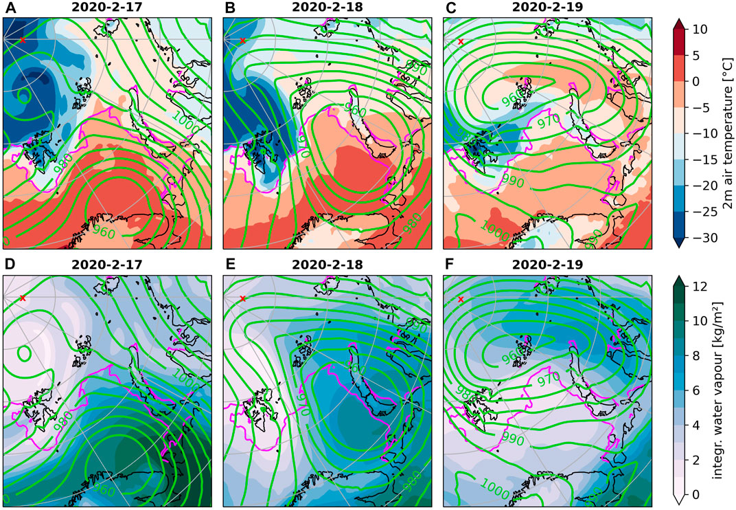
FIGURE 2. Daily means of 2-m air temperature (A–C) and integrated water vapour (IWV) (D–F) during cyclone 2 (17.2.2020—19.2.2020) based on the HIRHAM–NAOSIM simulation. Green contour lines represent daily mean sea level pressure (in steps of 5 hPa); pink lines indicate the position of the ice edge (15% SIC). The position of the RV Polarstern at the corresponding days is marked as red cross.

Both before and after this particular cyclone event, the BKS region was affected by another cyclone with comparatively similar intensity and track (Figure 1, Supplementary Figures S5, S6). The first of the three cyclones occurred during February 10–13 (in the following referred to as cyclone 1), crossed the central Barents Sea between February 11–12, and entered the central Arctic close to Franz Josef Land. The last of the three consecutive cyclones (in the following referred to as cyclone 3) occurred during February 21–25, entered the Barents Sea on February 22, and followed almost the same path as the second cyclone for most of its lifetime. However, in contrast to cyclone 2, it decayed quicker, i.e., one day earlier than cyclone 2, after reaching the central Arctic between Svalbard and Franz Josef Land.

The comparison of the nudged coupled model simulation with MOSAiC data demonstrates that the observed atmospheric variability in the central Arctic during this series of cyclones is captured well by the model (Supplementary Figure S2). With respect to larger spatial scales, the simulated patterns of 2-m air temperature and IWV over the BKS region agree with those of ERA5 (Supplementary Figure S1). This confirms the validity of the atmospheric forcing in the simulation.

3.2 Cyclone impacts on SEB

Analyzing the SEB for cyclone 2 (Figures 3A–C) reveals that starting with February 18, the advection of cold and dry air at the back side of the cyclone leads to a strong energy transfer from the ocean to the atmosphere in the Barents Sea. Over the open ocean, but also in parts of the marginal ice zone (MIZ), i.e., in the central Barents Sea and west of Svalbard, the SEB reaches values below −350 Wm⁻². On February 19, this advection of cold dry air further extends to the eastern Barents Sea. Comparing individual components of the SEB indicates that this intensification of the usually slightly negative wintertime SEB is almost exclusively driven by turbulent heat fluxes (Figures 3D–F). Changes in net longwave radiation associated with the cyclone passage (determined by an increase in longwave downward radiation) lead to a slightly less negative SEB in the Kara Sea and central Arctic (Figures 3G–I), but this signal does not reach the same order of magnitude as the negative SEB change due to turbulent heat fluxes.

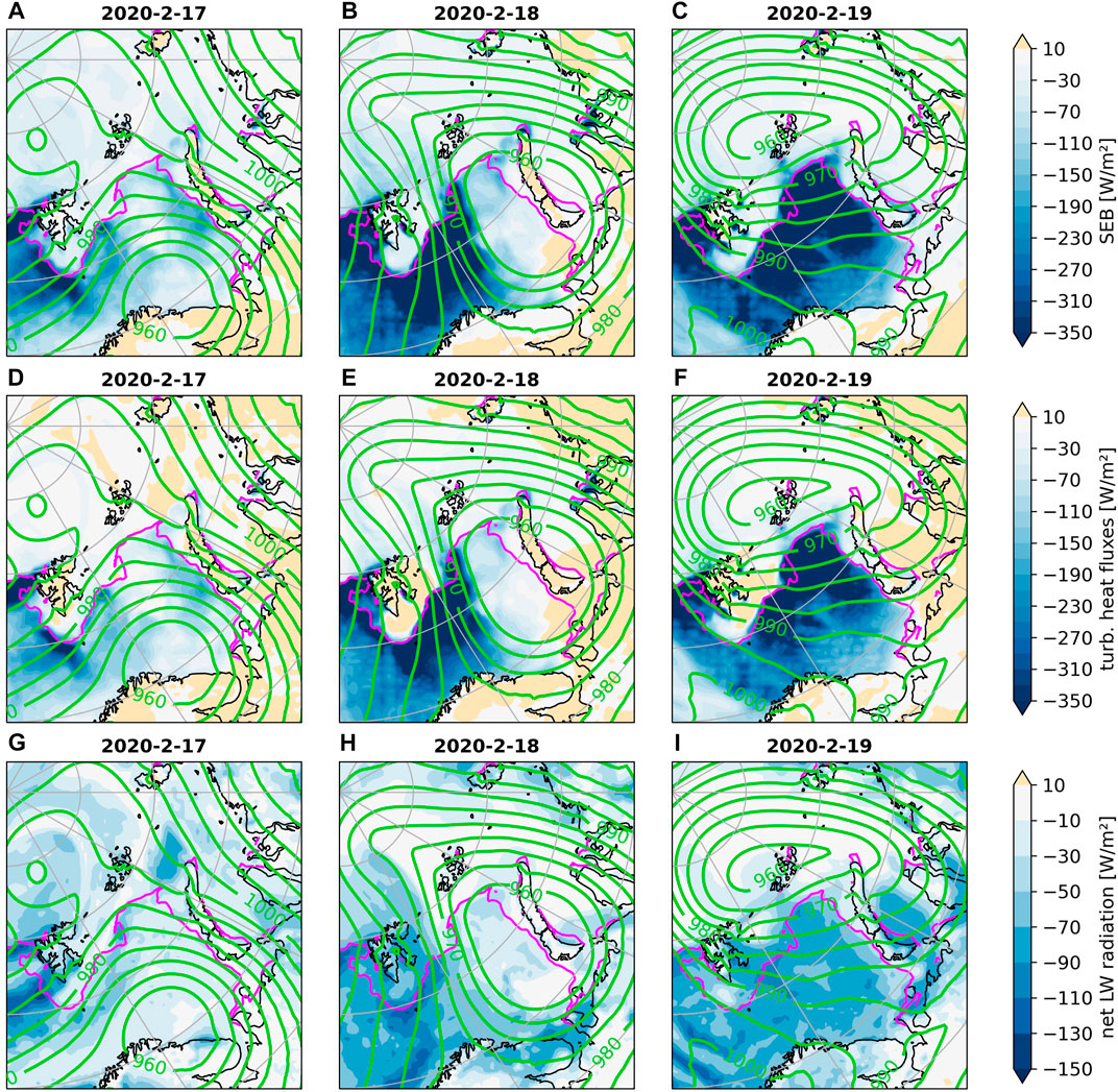
FIGURE 3. Daily means of atmospheric surface energy budget (SEB) (A–C), sum of atmospheric turbulent surface heat fluxes (D–F) and net longwave radiation (G–I) during cyclone 2 (17.2.20—19.2.20) based on the HIRHAM–NAOSIM simulation. Positive (negative) values indicate downward (upward) fluxes. Green contour lines represent daily mean sea level pressure (in steps of 5 hPa); pink lines indicate the position of the ice edge (15% SIC).

The SEB change during all three cyclone cases (Figure 3, Supplementary Figures S5, S6) is in contrast to reports on strong positive SEB changes (energy gain of the surface) in ice-covered grid-cells during an extreme cyclone in December 2015/January 2016 (Boisvert et al., 2016) and during the record Arctic cyclone in January 2022 (Blanchard-Wrigglesworth et al., 2022). For our presented mid-February 2020 case, only small patches of slightly positive SEB are found during a very few days, i.e., during cyclone 2 on February 18 southwest of Novaya Zemlya (Figure 3B) and during cyclone 1 on February 12 over the Barents Sea (Supplementary Figure S5). Apart from that, the SEB remains negative in ice-free grid-cells and is close to zero in ice-covered grid-cells. Since both the December 2015/January 2016 cyclone and the January 2022 cyclone entered the BKS close to Svalbard on a more northerly route than the Mid-February 2020 cyclones, it can be supposed that there is a strong variability in the surface impacts of individual cyclones depending on their track and presumably also on further cyclone properties.

3.3 Cyclone impacts on sea ice concentration (SIC)

As a next step, we analyze changes in SIC from directly before the start of the first cyclone passage to the end of the third one (from February 9 to February 25). Figure 4A shows that the sequence of cyclones causes a strong decrease (increase) in SIC in the eastern (western) part of the study domain, particularly in the MIZ. Strongest changes exceeding values of 50% are found in the vicinity of Novaya Zemlya and Svalbard. The simulated spatial pattern of SIC changes shows strong similarities to satellite observations of SIC contained in the ERA5 reanalysis (Supplementary Figure S3), which confirms the suitability of the coupled model simulation for our study.

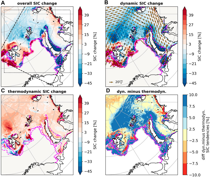
FIGURE 4. Overall SIC change during the whole sequence of cyclones (9.2.20-25.2.2020) (A), temporally integrated dynamic (advective plus rafting and ridging) SIC change as well as mean sea ice drift vectors (B), temporally integrated thermodynamic SIC change (C), and difference between absolute values of temporally integrated dynamic and thermodynamic SIC change (D) based on the HIRHAM–NAOSIM simulation. Solid (dashed) pink lines indicate the position of the ice edge (15% SIC) on 9.2.2020 (25.2.2020). Dashed (dotted) box in (A) indicates domain of spatially averaged SIC (SLP) changes in Section 3.5.

3.3.1 Dynamic and thermodynamic contributions

Figures 4B–D shows that dynamic mechanisms dominate the response of the sea ice cover to the sequence of cyclones. The above-mentioned decrease in SIC east of Novaya Zemlya is caused by northeastward ice drift towards the central Kara Sea (Figure 4B), triggered by the cyclone passages. At the same time, the increase in SIC in the western part of the study domain is related to a strong intensification of an existing southwesterly drift of sea ice around Svalbard towards the Fram Strait. In the MIZ as well as in the consolidated ice pack, the thermodynamic SIC response (Figure 4C) is widely anti-correlated to the dynamic SIC changes and thus partly compensates for the dynamic decrease of SIC.

The thermodynamic decrease in SIC south and (north)west of Svalbard is notable, since this region is affected by the advection of cold, dry air west of the cyclone centers (Figure 2, Supplementary Figures S5, S6). Such atmospheric conditions tend to promote increased ice growth, which does not fit to the simulated thermodynamic SIC decrease. A possible explanation is given by the enhanced southwestward advection of sea ice during the cyclone passages into regions with comparatively warm ocean water, with the thermodynamic SIC decrease being related to basal melting of sea ice rather than to atmospheric influence. This hypothesis is supported by a spatial pattern of comparatively strong upward oceanic surface heat fluxes in the presence of sea ice (Supplementary Figure S7), which shows similarities to the spatial pattern of thermodynamic SIC decrease (Figure 4C). This hypothesis is further backed up by recent findings of Duarte et al. (2020), who report on the importance of oceanic heat content for the melting of sea ice near Svalbard, particularly in combination with storms.

The difference between integrated dynamic and thermodynamic SIC changes (Figure 4D) confirms that dynamic SIC changes dominate (difference $>0$) the response of the sea ice cover to the analyzed series of cyclones not only close to the ice edge, but also in large parts of the consolidated ice pack. The clear dominance of dynamic mechanisms south and east of Novaya Zemlya indicates that the cyclone-related advection of warm and moist air into this region does not play a substantial role for SIC. For our cyclone case, only in the western Barents Sea, particularly south (east) of Svalbard, thermodynamics are (partly) of high importance for the SIC changes. There, northerly winds at the western flank of the cyclones push the ice edge southward and, at the same time, cold and dry air is advected from the central Arctic (Figure 1; Figure 2; Supplementary Figures S5, S6). This leads to refreezing of leads and openings in the sea ice cover that are caused by the southward drift of ice due to the cyclonic wind anomalies. In general, the role of thermodynamics during the cyclone passages seems to be limited to this refreezing in regions that have experienced dynamic decrease of SIC. Hereby, the advection of warm and moist air east of the cyclone tracks might explain why such refreezing is occurring only to a very limited extent south and east of Novaya Zemlya, while it is stronger close to the ice edge in the central Barents Sea and north of Svalbard (Figure 4C).

Further it should be mentioned that to some degree, thermodynamic SIC increases due to refreezing are not a direct consequence of the cyclone passages only, but would happen anyway in Arctic winter due to the seasonal sea ice growth. A rough estimate of this effect can be obtained from the study of Aue et al. (2022), who compared cyclone related SIC changes on daily to weekly timescales with a non-cyclone reference obtained from ERA5 data for the period 2000–2020 for Arctic winter (December to February). For this, weekly SIC changes ranged from 1 to 10% in the BKS in the non-cyclone reference. Consequently, the strong thermodynamic SIC increases in the western part of the study domain (around Svalbard) are larger than usually in winter, and the non-existing SIC growth south and east of Novaya Zemlya is unusual compared to non-cyclone conditions.

To gain further insights into the variability of the cyclone impacts on sea ice, we quantify the contributions of the individual cyclones one to three to the accumulated signal in the change of SIC. Accordingly, Figure 5 shows the SIC change simulated during each of the three cyclone passages. In order to analyze whether the apparent impacts of a cyclone may include contribution by the preceding cyclone, we make use of the fact that three cyclones with a similar track travelled across the BKS in a comparatively short time period.

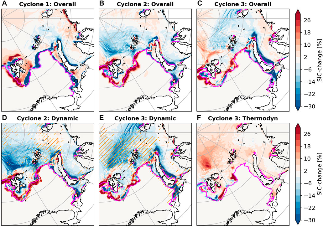
FIGURE 5. SIC change during cyclone 1 (9.2.—13.2.2020) (A), cyclone 2 (15.2.—20.2.2020) (B) and cyclone 3 (20.2.—25.2.2020) (C) as well as temporally integrated dynamic SIC changes for cyclone 2 (D) and cyclone 3 (E) and temporally integrated thermodynamic SIC changes during cyclone 3 (F). Orange hatching indicates grid-cells that have lost at least 5 cm of SIT during the previous cyclone passage(s). All based on the HIRHAM–NAOSIM simulation. Pink lines indicate the position of the ice edge (15% SIC) at the start of each cyclone passage.

While the SIC impacts of cyclones 2 and 3 are similar, there are differences to the SIC change during the first of the three cyclones (Figures 5A–C). For the latter two cyclones, a SIC decrease south and east of Novaya Zemlya is accompanied by a SIC increase extending along the ice edge from the central Barents Sea to the west of Svalbard. While the SIC decrease is slightly stronger for cyclone 3, the SIC increase is slightly stronger for cyclone 2. Nonetheless, the patterns are similar. In contrast, cyclone 1 shows a strong SIC decrease of more than 30% not only in the eastern Barents Sea and Kara Sea but also in the central Barents Sea and southeast of Svalbard. In addition, cyclones 2 and 3 have an almost identical track for large parts of their lifetime, while the track of cyclone 1 is somewhat different (Figure 1). This suggests that the exact location of a cyclones’ track and its orientation relative to the ice edge is crucial for the resulting impact on SIC. This hypothesis is supported when comparing our findings with the winter cyclone cases analyzed by Boisvert et al. (2016) and Blanchard-Wrigglesworth et al. (2022). In fact, the track of their cyclones resembles that of cyclone 1 more than those of cyclone 2 and 3, and the same is true with respect to the SIC changes in the BKS, which mostly consist of a SIC decrease.

3.3.2 Preconditioning and time scale

It has been shown that cyclone impacts on SIC are amplified when preconditioned by locally low to medium SIC (Aue et al., 2022). Additionally, it can be assumed that also SIT plays a role for the susceptibility of the sea ice cover to atmospheric forcing during cyclone passages (Zhang et al., 2012; Rheinlaender et al., 2022). To account for both of these effects while investigating a possible relevance of previous cyclone passages for the impact of the current cyclone on SIC, we analyze the role of grid-cell mean sea ice thickness (SIT), also referred to as sea ice volume per unit area.

Based on the spatial patterns of SIT decrease during previous cyclone passages, it seems that this preconditioning of the ice cover during cyclone 2 influenced the SIC changes during cyclone 3. Particularly in the consolidated ice pack, regions with dynamically-driven decrease of SIC during cyclone 3 (Figure 5E) widely correspond to regions that have experienced SIT decrease during the previous cyclones. In contrast, the spatial patterns of dynamic SIC changes during cyclone 2 (Figure 5D) do not fit to those of SIT decrease during cyclone 1.

A possible explanation is that cyclone 1 did not stay as long over the consolidated ice pack as the more intense cyclone 2, which remained north of Svalbard and Franz Josef Land for around 2 days before decaying (Figure 1). The matching patterns of SIC changes during cyclone 3 and preconditioning during cyclone 2 might as well just be a coincidence or related to the fact that both cyclones had a very similar track and presumably exerted a similar wind forcing on the sea ice cover. Consequently, detailed future research is needed to more convincingly conclude about the effect of preconditioning of the sea ice for following cyclone passages.

North of Svalbard, the SIC was (temporary) decreased by up to 20% during cyclone 2 (Figure 5B), which was the most intense of the three cyclones. At the same grid-cells, thermodynamic SIC increase occurred during cyclone 3 due to refreezing (Figure 5F). This increase in SIC during cyclone 3 would not have been possible without the preceding cyclone 2, because SIC would have presumably been close to 100% in that part of the Arctic Ocean in February. This constraint of typically high SIC values in Arctic winter might help to explain why dynamic SIC changes are more pronounced than their thermodynamic counterparts during this series of cyclone events for large parts of the study domain.

Another factor that might dampen the thermodynamic SIC changes during the presented series of cyclones is time. Thermodynamic surface impacts via LWD can last 1–2 weeks (Park et al., 2015). Specifically, Aue et al. (2022) showed that the SIC increase following cyclone passages in the Barents Sea in winter lasts up to 5–7 days. For cyclones 1 and 2, this amount of time was not available until the next cyclone passage started. For cyclone 3–which was not immediately followed by another cyclone–it is clearly visible that the magnitude of the thermodynamic SIC changes as well as their relative importance compared to the dynamic SIC changes increase with time (Figure 6). During the passage of cyclone 3, thermodynamic SIC changes are limited to only a few locations in the study domain (Figure 6A) and are mostly less pronounced than their dynamic counterparts (Figure 6D). The only exception is found north of Svalbard, but the comparatively strong refreezing in this region is related to the preceding cyclone passage as discussed earlier.

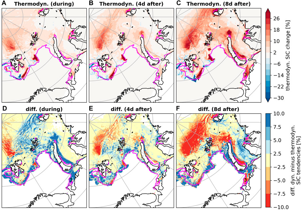
FIGURE 6. Temporally integrated thermodynamic SIC change (A–C) and difference between absolute values of temporally integrated dynamic and thermodynamic SIC change (D–F) during (20.2.—24.2.2020), shortly after (24.2.20—28.2.2020) and for a longer period after (24.2.—3.3.2020) cyclone 3 based on the HIRHAM–NAOSIM simulation. Pink lines indicate the position of the ice edge (15% SIC) at the start of the cyclone passage.

During the 4 days that immediately follow the cyclone passage, a broader region, which includes areas north of Svalbard and Franz Josef Land, shows an accumulated thermodynamic SIC increase of 10–20% (Figure 6B). Consequently, thermodynamics also become slightly more important for the overall SIC change on that time scale (Figure 6E). If the time period is further extended to 8 days following the cyclone passage, a strong thermodynamic SIC increase is found in the central Arctic, in the northern Kara Sea as well as south and east of Novaya Zemlya (Figure 6C). On this time scale, thermodynamic SIC changes even outweigh their dynamic counterparts for large parts of the study domain (Figure 6F). To some degree, this thermodynamic SIC increase with time is just a consequence of seasonal sea ice growth in winter. This effect can be roughly estimated to 1–10% SIC increase in 1 week in the BKS for non-cyclone conditions (see Section 3.3.1). This indicates that especially the strong (accumulated) thermodynamic SIC increases of more than 20% in 8 days north of Franz Josef Land, in the northern Kara Sea and around Novaya Zemlya following cyclone 3 (Figure 6C) are much larger than usually for Arctic winter and thus can be partly attributed to the cyclone passage.

In conclusion, our analysis of SIC changes on different time scales suggests that during the cyclone passage dynamics clearly outweigh thermodynamics, while it is partly the other way around for the days following the cyclone, provided that there is not another cyclone passage taking place in quick succession. For cyclone 3, this results in a regional difference of SIC increase (decrease) west (east) of the cyclone track during the cyclone passage, as well as in strong increases in SIC in the whole MIZ after the cyclone passage (Supplementary Figure S8).

3.4 Cyclone impacts on sea ice thickness (SIT)

In this section, we extend our analysis of cyclone impacts to dynamic and thermodynamic changes in SIT, which have been rarely studied. A comparison of the simulated mean SIT from February 9 to 22 February 2020 with observations based on CryoSat-2 and SMOS satellite data (Ricker et al., 2017b) demonstrates that the spatial distribution of regions with relatively thin ice and relatively thick ice is captured by the model (Supplementary Figures S4A, B). However, it should be noted that the simulated SIT field is generally too smooth, leading to an underestimation of SIT in the central Arctic and to an overestimation of SIT in the Kara Sea and some parts of the marginal ice zone.

Simulated SIT changes during the cyclone passages mainly consist of a decrease in SIT east of Novaya Zemlya and an increase in SIT northwest of Svalbard (Figure 7A). Generally, there are some differences between the simulated and observed SIT response to the cyclone passages (Supplementary Figures S4C, D), which should be kept in mind when interpreting the results. However, the previously described main features around Novaya Zemlya and Svalbard are consistent in both datasets, which confirms the applicability of the simulation for this case study.

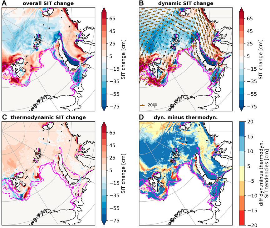
FIGURE 7. Overall SIT change during the whole sequence of cyclones (9.2.20-25.2.2020) (A), temporally integrated dynamic SIT change as well as mean sea ice drift vectors (B), temporally integrated thermodynamic SIT change (C), and difference between absolute values of temporally integrated dynamic and thermodynamic SIT change (D) based on the HIRHAM–NAOSIM simulation. Solid (dashed) pink lines indicate the position of the ice edge (15% SIC) on 9.2.2020 (25.2.2020).

3.4.1 Dynamic and thermodynamic contributions

The results show that changes in SIT during the series of the three cyclone passages are–similarly to changes in SIC–dominated by dynamic mechanisms (Figure 7). Sea ice is mainly moved from the eastern coast of Novaya Zemlya towards the central Kara Sea as well as from the central Arctic (north of Franz Josef Land) towards Svalbard during the cyclone events (Figure 7B). This is consistent with the cyclonic wind anomalies that can be expected based on the cyclone tracks. The dominance of dynamics for SIT changes (Figure 7D) is even more pronounced than for SIC changes. This is in agreement with results by Clancy et al. (2022), who analyzed cyclone-related changes in ice thickness on a cyclone-centered grid in winter utilizing model simulations.

With respect to thermodynamic changes in SIT, comparatively strong increases can be found north (up to 20 cm) as well as south and east (up to 50 cm) of Svalbard, while a decrease occurs southwest of Svalbard (Figure 7C). This pattern closely resembles the thermodynamic SIC changes presented in Figure 4. South and east of Novaya Zemlya, no thermodynamic increases in SIT are found during the cyclone passages, and at a very few locations even a minor thermodynamic decrease in SIT is visible (Figure 7C). This is presumably related to a stalling of ice growth caused by the advection of warm and moist air masses at the eastern flank of the cyclones and subsequent impacts on SEB. However, the overall magnitude of this stalling in sea ice growth is rather small, as estimated by comparing the growth rates in the eastern and western part of the study domain (differences between 0 cm and 20 cm over more than 2 weeks). Consequently, thermodynamics do not play a large role for the overall changes in SIT during this sequence of cyclones, which are clearly dominated by dynamics (Figure 7D).

3.4.2 Preconditioning and time scale

Since our analysis of changes in SIC demonstrated a large sensitivity of the thermodynamic effect to the time scale (Section 3.3.2), we further analyze this for changes in SIT (Figure 8).

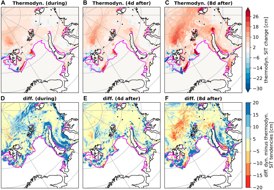
FIGURE 8. Temporally integrated thermodynamic SIT change (A–C) and difference between absolute values of temporally integrated dynamic and thermodynamic SIT change (D–F) during (20.2.—24.2.2020), shortly after (24.2.20—28.2.2020) and for a longer period after (24.2.—3.3.2020) cyclone 3 based on the HIRHAM–NAOSIM simulation. Pink lines indicate the position of the ice edge (15% SIC) at the start of the cyclone passage.

Similarly to SIC (Figure 6), the thermodynamic SIT change gets stronger with time (Figures 8A–C) and simultaneously becomes more important relative to its dynamic counterpart (Figures 8D–F). This is because the thermodynamic ice growth is relatively slow compared to the dynamic SIT change. Particularly north of Svalbard and Franz Josef Land as well as close to Novaya Zemlya, thermodynamic SIT increase is enhanced during the 8 days that follow cyclone 3 (Figure 8C), because the now thinner ice (due to dynamics) freezes faster and produces more ice than it would have been without the cyclone passage. Nonetheless, thermodynamics do not reach a comparatively strong importance for SIT as for SIC (Figures 8F vs. Figures 6F). For large parts of the Barents and Kara Seas, dynamics remain the dominating factor also on longer time scales following the cyclone passage. A notable result is that in the southern Kara Sea along the coast of Siberia almost no ice thickness growth occurs during the 8 days following the last cyclone passage (Figure 8C). In contrast to SIC, this cannot be explained by the constraining boundary condition that the SIC at these grid-cells is almost 100%. At the same time, this region was also most strongly affected by the advection of warm and moist air masses in the cyclone’s eastern sector. This leaves the open question how long the cyclone-induced stalling of ice growth is actually lasting.

3.5 Context to other cyclone cases during the MOSAiC winter

To generalize the results from this case study and move towards more solid conclusions on dynamic and thermodynamic contributions to cyclone-driven sea ice changes, we extend our analysis period to the whole winter of our selected year, specifically to January-March 2020.

The time series of the daily SLP averaged over the BKS region (Figure 9, domain shown in Figure 4) is an indicator for cyclone activity in the BKS. The figure highlights the main cyclone cases during the period and their tracks are shown in the Supplementary Figure S9. The cyclone at the beginning of February affected the western BKS around Svalbard for several days starting at February 2, before moving southeastward through the Barents Sea while decaying. The mid-February case of three successive cyclones was discussed in detail in Section 3. The two March events affected the BKS for several days each, with one cyclone taking a similar path as the mid-February cases (through the southern Barents Sea to the Kara Sea into the central Arctic) and the other cyclone entering the BKS on a more northerly track close to Svalbard. They occurred one after the other at intervals of approximately 1 week.

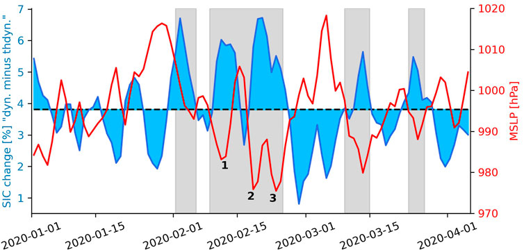
FIGURE 9. Difference of “absolute value of dynamic SIC change” minus “absolute value of thermodynamic SIC change” (blue line), both integrated over 5 days and averaged over the BKS (domain shown in Figure 4). Blue filled areas indicate the anomaly compared to the Jan. to March 2020 mean (black dotted line). Red line indicates SLP averaged over the BKS (domain shown in Figure 4). Grey areas highlight the main cyclone cases in Jan. to March 2020, numbers indicate the three cyclones analyzed in Section 3.

To discuss the importance of dynamics and thermodynamics for the related SIC changes, we follow the approach of Section 3 and show in Figure 9 the time series of the difference between the absolute value of the temporally integrated dynamic SIC change and its thermodynamic counterpart, integrated over 5 days and averaged over the BKS region. Based on our previous analysis, 5 days are an appropriate time period to capture the SIC impacts of individual cyclones (see, e.g., Figure 5).

First of all, the SIC difference is positive throughout the 3 months with a mean value of approximately 4% (indicated by the black dashed line in Figure 9). This indicates that for the complete January-March 2020, dynamic SIC changes dominate the overall SIC changes in the BKS region. This is in accordance with our previous analysis (Figure 4). Importantly, there is a significant temporal variability in the SIC difference, and thus in the relative importance of dynamics and thermodynamics, often associated with changes in SLP as indicated by the red line in Figure 9.

In agreement with our previous analysis of three consecutive cyclones in mid-February (Figure 4; Figure 6), the SIC difference is shifted towards more positive values (compared to the mean value) during these cyclone passages. This indicates a dominance of dynamic over thermodynamic contributions for up to 2 weeks. After the last of the three cyclones however, a shift towards smaller values indicates an increasing relative importance of thermodynamic processes for SIC changes, which lasts for about 2 weeks with comparatively high air pressure. A similar phase of higher relative importance of thermodynamic SIC changes under high air pressure conditions can be found end of January.

The process of enhanced dynamic SIC changes during and enhanced thermodynamic SIC changes after a cyclone passage is also found for the two cyclone cases that affected the BKS in March 2020 (Figure 9). After both of these cyclones, it took approximately 1 week before the next cyclone arrived in the BKS. Consequently, there was time for thermodynamic SIC changes to take the lead. This supports the hypothesis raised in Section 3 that enhanced thermodynamic SIC changes can take place after cyclone passages if not another cyclone follows in quick succession. In accordance with this, Figure 9 does not show a period of enhanced thermodynamic SIC changes after the passage of the early February cyclone case. This can be related to the fact the series of the mid-February cyclones started shortly afterwards.

4 Discussion and conclusion

The main objective of our study is to quantify cyclone-related dynamic and thermodynamic impacts on the sea ice cover in order to clarify which of these mechanisms is more important in Arctic winter. It turns out that for the presented sequence of three intense cyclones in February 2020 dynamic contributions are the dominating mechanism for changes in SIC and SIT. Especially cyclone-related decreases in SIC and SIT are almost exclusively driven by dynamic processes. The role of thermodynamics is limited to drive increases in SIC and SIT due to refreezing of leads after the cyclone passages, and to enhance ice growth under cold and dry conditions on the cyclones’ western flank. However, after the passing of the cyclones the increased thermodynamic ice growth of the now thinner ice continues, while the dynamic changes only have an immediate effect during the cyclones passing.

For SIT, our results are in accordance with findings by Clancy et al. (2022), who emphasized that dynamic processes are dominant for this quantity in Arctic winter. Apart from that, our findings are partly in contradiction to recent studies by Cai et al. (2020) and Schreiber and Serreze. (2020), who found evidence that thermodynamics are the more important factor of the cyclones’ impact on sea ice in the cold season. On the one hand, this could be related to the fact that the presented work is a case study of three particular cyclones. Obviously, there can be differences in cyclone impacts on sea ice for different cases. However, since the tracks of the chosen cyclone cases closely resemble the main cyclone track in the Atlantic sector of the Arctic Ocean in winter, we argue that the sequence of storms presented here is representative. On the other hand, our findings reveal that the considered time scale has a strong impact on the ratio of dynamic and thermodynamic sea ice changes. This can explain differences between studies. A detailed analysis of the last of the three presented cyclones emphasizes that thermodynamic sea ice changes become more important on a longer time scale (weekly) following the cyclone passage. This agrees with results by Park et al. (2015) for sea ice changes related to moisture intrusion events. For the here presented mid-February case, thermodynamics locally outweigh the importance of dynamics on timescales of about 1 week following the cyclone passage, mostly in the consolidated ice pack and less frequently in the MIZ close to the ice edge, where dynamic sea ice changes are most pronounced.

A comparison of the mid-February case with other cyclone cases from January to March 2020 suggests that an initial dominance of dynamically caused SIC changes, followed by enhanced thermodynamic impacts, is typical of cyclone passages in the BKS in winter. Further analysis covering more cases from different years is necessary to confirm this hypothesis. Recent statistical studies have reported on cyclone-related increases in SIC in the Arctic winter (Schreiber and Serreze, 2020; Aue et al., 2022), mostly taking place a couple of days after the cyclone passage. If our findings are representative for winter cyclones, this would suggest that the reported SIC increases are likely driven by thermodynamics. In that case, dynamical mechanisms could reasonably explain the strong SIC changes initially taking place during most cyclones by redistributing the sea ice, while enhanced ice growth in leads in the more consolidated ice pack offers an explanation for the positive ice mass balance impact after the cyclone passage.

It should be noted that this mechanism only works in regions with cold surface waters. For instance, if sea ice is advected over warmer Atlantic water south of the polar front in the Barents Sea or over the Yermack Plateau north of Svalbard, the ice will be subject to basalt melt. If cyclones mix up warmer sub-surface waters, this can further change the regions with stronger oceanic heat flux impact (Duarte et al., 2020). Another factor that seems to restrict the thermodynamic increase in SIC after the cyclones is the time available until the following cyclone passage. Decomposing the sea ice changes for the whole sequence of cyclone events reveals that dynamics can be the dominating mechanism for changes in SIC and SIT on time scales of more than 2 weeks if cyclone passages occur in quick succession.

Apart from the importance of the timing of cyclone passages, our findings further indicate that comparatively minor differences in the location of a cyclone track can result in strong differences in the cyclone impact on the sea ice cover, particularly in the MIZ. Recently, Lukovich et al. (2021) came to similar conclusions regarding the importance of the exact position (and timing) of cyclones when analyzing the impacts of extreme summer cyclones on Arctic sea ice. In addition to a cyclone’s timing and track, further factors, such as its intensity or the source region of its air masses, presumably contribute to the variability of the impacts of individual cyclones on sea ice. Furthermore, a high spatiotemporal resolution is crucial for capturing cyclone intensification rates and maximum intensity (e.g., Parker et al., 2022). Accordingly, a relatively coarse atmosphere resolution (1/4° in our model as well as in ERA5) has its limitation in this regard. In conclusion, identifying the key parameters that determine the impact of a specific cyclone on sea ice is not only a complex but also an important research task, particularly in order to make reliable predictions on future cyclone impacts on sea ice in a warming Arctic.

Data availability statement

Publicly available datasets were analyzed in this study. This data can be found here: HIRHAM-NAOSIM data are available at the tape archive of the German Climate Computing Center (DKRZ): https://www.dkrz.de/en/systems/datenarchiv. One needs to register at DKRZ to get a user account. We will also make the data available via Swift on request: https://www.dkrz.de/up/systems/swift. ERA5 data are available on the Copernicus Climate Change Service Climate Data Store: https://cds.climate.copernicus.eu/cdsapp#!/dataset/reanalysis-era5-single-levels?tab&equals form. 10-m meteorological flux tower measurements from MOSAiC are available at the Arctic Data Center: https://arcticdata.io/catalog/view/doi:10.18739/A2VM42Z5F. Measurements at the Atmospheric Surface Flux Stations from MOSAiC are available at the Arctic Data Center: https://arcticdata.io/catalog/view/doi:10.18739/A20C4SM1J; https://arcticdata.io/catalog/view/doi:10.18739/A2CJ87M7G; https://arcticdata.io/catalog/view/doi:10.18739/A2445HD46. HATPRO data from MOSAiC are available at PANGAEA: https://doi.pangaea.de/10.1594/PANGAEA.941389.

Author contributions

All authors contributed to conception and design of the study. WD provided the database of the study consisting of the coupled model simulation. LA, LR, and AR were in charge of carrying out the scientific analysis and creating the figures. LA, AR, and WD wrote the first draft of the manuscript. All authors contributed to manuscript revision, read, and approved the submitted version.

Funding

LA, WD, GS, and AR acknowledge the funding by the Deutsche Forschungsgemeinschaft (DFG, German Research Foundation) project 268020496 TRR 172, within the Transregional Collaborative Research Center “ArctiC Amplification: Climate Relevant Atmospheric and SurfaCe Processes, and Feedback Mechanisms (AC)³”. WD, PU, TV, and AR acknowledge the funding by the European Union’s Horizon 2020 research and innovation framework programme under Grant agreement no. 101003590 (PolarRES project).

Acknowledgments

We thank Matthias Buschmann from the University of Bremen for providing the formula of the seasonalcycle of carbon dioxide used in HIRHAM–NAOSIM version 2.2. Some of the data used in this study were produced as part of the international Multidisciplinary drifting Observatory for the Study of the Arctic Climate (MOSAiC) project with the tag MOSAiC20192020. We thank all persons involved in the expedition of the RV Polarstern during MOSAiC in 2019–2020 (AWI PS122 00) as listed by Nixdorf et al. (2021). We further thank three anonymous reviewers for their helpful feedback. This work used resources of the Deutsches Klimarechenzentrum (DKRZ) under project ID aa0049. We acknowledge support by the Open Access Publication Funds of Alfred-Wegener-Institut Helmholtz-Zentrum für Polar-und Meeresforschung.

Conflict of interest

The authors declare that the research was conducted in the absence of any commercial or financial relationships that could be construed as a potential conflict of interest.

Publisher’s note

All claims expressed in this article are solely those of the authors and do not necessarily represent those of their affiliated organizations, or those of the publisher, the editors and the reviewers. Any product that may be evaluated in this article, or claim that may be made by its manufacturer, is not guaranteed or endorsed by the publisher.

Supplementary material

The Supplementary Material for this article can be found online at: https://www.frontiersin.org/articles/10.3389/feart.2023.1112467/full#supplementary-material

References

Aue, L., Vihma, T., Uotila, P., and Rinke, A. (2022). New insights into cyclone impacts on Sea Ice in the atlantic sector of the Arctic Ocean in winter. Geophys. Res. Lett. 49, e2022GL100051. doi:10.1029/2022GL100051
Blanchard-Wrigglesworth, E., Webster, M., Boisvert, L., Parker, C., and Horvat, C. (2022). Record arctic cyclone of january 2022: Characteristics, impacts, and predictability. J. Geophys. Res. Atmos. 127, e2022JD037161. doi:10.1029/2022JD037161
Boisvert, L., Petty, A., and Stroeve, J. (2016). The impact of the extreme winter 2015/16 Arctic cyclone on the Barents-Kara seas. Mon. Weather Rev. 144, 4279–4287. doi:10.1175/MWR-D-16-0234.1
Cai, L., Alexeev, V. A., and Walsh, J. E. (2020). Arctic sea ice growth in response to synoptic- and large-scale atmospheric forcing from CMIP5 models. J. Clim. 33, 6083–6099. doi:10.1175/JCLI-D-19-0326.1
Clancy, R., Bitz, C. M., Blanchard-Wrigglesworth, E., McGraw, M. C., and Cavallo, S. M. (2022). A cyclone-centered perspective on the drivers of asymmetric patterns in the atmosphere and sea ice during Arctic cyclones. J. Clim. 35, 1–47. doi:10.1175/JCLI-D-21-0093.1
Cox, C., Gallagher, M., Shupe, M., Persson, O., and Solomon, A. (2021a). 10-meter (m) meteorological flux tower measurements (level 1 raw), multidisciplinary drifting observatory for the study of arctic climate (MOSAiC), central arctic. Arct. Data Cent. doi:10.18739/A2VM42Z5F
Cox, C., Gallagher, M., Shupe, M., Persson, O., and Solomon, A. (2021b). Atmospheric surface flux station #30 measurements (level 1 raw), multidisciplinary drifting observatory for the study of arctic climate (MOSAiC), central arctic. Arct. Data Cent. doi:10.18739/A20C4SM1J
Cox, C., Gallagher, M., Shupe, M., Persson, O., and Solomon, A. (2021c). Atmospheric surface flux station #50 measurements (level 1 raw), multidisciplinary drifting observatory for the study of arctic climate (MOSAiC), central arctic. Arct. Data Cent. doi:10.18739/A2445HD46
Dorn, W., Dethloff, K., and Rinke, A. (2009). Improved simulation of feedbacks between atmosphere and sea ice over the Arctic Ocean in a coupled regional climate model. Ocean. Model. 29, 103–114. doi:10.1016/j.ocemod.2009.03.010
Dorn, W., Rinke, A., Köberle, C., Dethloff, K., and Gerdes, R. (2019). Evaluation of the sea-ice simulation in the upgraded version of the coupled regional atmosphere-ocean-sea ice model HIRHAM–NAOSIM 2.0. Atmosphere 10, 431. doi:10.3390/atmos10080431
Duarte, P., Sundfjord, A., Meyer, A., Hudson, S. R., Spreen, G., and Smedsrud, L. H. (2020). Warm Atlantic water explains observed sea ice melt rates north of Svalbard. J. Geophys. Res. Oceans 125, e2019JC015662. doi:10.1029/2019JC015662
Graham, R. M., Itkin, P., Meyer, A., Sundfjord, A., Spreen, G., Smedsrud, L. H., et al. (2019). Winter storms accelerate the demise of sea ice in the Atlantic sector of the Arctic Ocean. Sci. Rep. 9, 9222. doi:10.1038/s41598-019-45574-5
Gultepe, I., Sharman, R., Williams, P. D., Zhou, B., Ellrod, G., Minnis, P., et al. (2019). A review of high impact weather for aviation meteorology. Pure Appl. Geophys. 176, 1869–1921. doi:10.1007/s00024-019-02168-6
Haas, C. (2017). Sea ice thickness distribution. New York: John Wiley and Sons, Ltd. doi:10.1002/9781118778371.ch2
Hersbach, H., Bell, B., Berrisford, P., Hirahara, S., Horányi, A., Muñoz-Sabater, J., et al. (2020). The ERA5 global reanalysis. Q. J. R. Meteorol. Soc. 146, 1999–2049. doi:10.1002/qj.3803
Hibler, W. D. (1979). A dynamic thermodynamic sea ice model. J. Phys. Oceanogr. 9, 815–846. doi:10.1175/1520-0485(1979)009⟨0815:ADTSIM⟩2.0.CO;2
Inoue, J. (2021). Review of forecast skills for weather and sea ice in supporting Arctic navigation. Polar Sci. 27, 100523. doi:10.1016/j.polar.2020.100523
Itkin, P., Spreen, G., Cheng, B., Doble, M., Girard-Ardhuin, F., Haapala, J., et al. (2017). Thin ice and storms: Sea ice deformation from buoy arrays deployed during N-ICE2015. J. Geophys. Res. Oceans 122, 4661–4674. doi:10.1002/2016JC012403
Koo, Y., Lei, R., Cheng, Y., Cheng, B., Xie, H., Hoppmann, M., et al. (2021). Estimation of thermodynamic and dynamic contributions to sea ice growth in the central Arctic using ICESat-2 and MOSAiC SIMBA buoy data. Remote Sens. Environ. 267, 112730. doi:10.1016/j.rse.2021.112730
Kriegsmann, A., and Brümmer, B. (2014). Cyclone impact on sea ice in the central Arctic Ocean: A statistical study. Cryosphere 8, 303–317. doi:10.5194/tc-8-303-2014
Kwok, R. (2018). Arctic sea ice thickness, volume, and multiyear ice coverage: Losses and coupled variability (1958–2018). Environ. Res. Lett. 13, 105005. doi:10.1088/1748-9326/aae3ec
Liu, Z., Risi, C., Codron, F., Jian, Z., Wei, Z., He, X., et al. (2022). Atmospheric forcing dominates winter Barents-Kara sea ice variability on interannual to decadal time scales. Proc. Natl. Acad. Sci. 119, e2120770119. doi:10.1073/pnas.2120770119
Lukovich, J. V., Stroeve, J. C., Crawford, A., Hamilton, L., Tsamados, M., Heorton, H., et al. (2021). Summer extreme cyclone impacts on Arctic sea ice. J. Clim. 34, 1–54. doi:10.1175/JCLI-D-19-0925.1
Meier, W. N., and Stroeve, J. (2022). An updated assessment of the changing Arctic sea ice cover. Oceanography 35, 10–19. doi:10.5670/oceanog.2022.114
Nixdorf, U., Dethloff, K., Rex, M., Shupe, M., Sommerfeld, A., Perovich, D. K., et al. (2021). MOSAiC extended acknowledgement. Version 1 ZENODO. doi:10.5281/zenodo.5541624
Park, H. S., Lee, S., Son, S. W., Feldstein, S. B., and Kosaka, Y. (2015). The impact of poleward moisture and sensible heat flux on Arctic winter sea ice variability. J. Clim. 28, 5030–5040. doi:10.1175/JCLI-D-15-0074.1
Parker, C. L., Mooney, P. A., Webster, M. A., and Boisvert, L. N. (2022). The influence of recent and future climate change on spring Arctic cyclones. Nat. Commun. 13, 6514. doi:10.1038/s41467-022-34126-7
Petty, A. A., Holland, M. M., Bailey, D. A., and Kurtz, N. T. (2018). Warm Arctic, increased winter sea ice growth? Geophys. Res. Lett. 45, 12922–12930. doi:10.1029/2018GL079223
Rampal, P., Weiss, J., and Marsan, D. (2009). Positive trend in the mean speed and deformation rate of Arctic sea ice, 1979–2007. J. Geophys. Res. Oceans 114, C05013. doi:10.1029/2008JC005066
Renfrew, I. A., Barrell, C., Elvidge, A. D., Brooke, J. K., Duscha, C., King, J. C., et al. (2021). An evaluation of surface meteorology and fluxes over the Iceland and Greenland Seas in ERA5 reanalysis: The impact of sea ice distribution. Q. J. R. Meteorol. Soc. 147, 691–712. doi:10.1002/qj.3941
Rheinlaender, J. W., Davy, R., Ólason, E., Rampal, P., Spensberger, C., Williams, T. D., et al. (2022). Driving mechanisms of an extreme winter sea ice breakup event in the Beaufort Sea. Geophys. Res. Lett. 49, e2022GL099024. doi:10.1029/2022GL099024
Ricker, R., Hendricks, S., Girard-Ardhuin, F., Kaleschke, L., Lique, C., Tian-Kunze, X., et al. (2017a). Satellite-observed drop of Arctic sea ice growth in winter 2015–2016. Geophys. Res. Lett. 44, 3236–3245. doi:10.1002/2016GL072244
Ricker, R., Hendricks, S., Kaleschke, L., Tian-Kunze, X., King, J., and Haas, C. (2017b). A weekly Arctic sea-ice thickness data record from merged CryoSat-2 and SMOS satellite data. Cryosphere 11, 1607–1623. doi:10.5194/tc-11-1607-2017
Rinke, A., Cassano, J. J., Cassano, E. N., Jaiser, R., and Handorf, D. (2021). Meteorological conditions during the MOSAiC expedition: Normal or anomalous? Elem. Sci. Anth. 9, 00023. doi:10.1525/elementa.2021.00023
Rinke, A., Maturilli, M., Graham, R., Matthes, H., Handorf, D., Cohen, L., et al. (2017). Extreme cyclone events in the Arctic: Wintertime variability and trends. Environ. Res. Lett. 12, 094006. doi:10.1088/1748-9326/aa7def
Schreiber, E., and Serreze, M. (2020). Impacts of synoptic-scale cyclones on Arctic seasea-ice concentration: A systematic analysis. Ann. Glaciol. 61, 139–153. doi:10.1017/aog.2020.23
Serreze, M. C., and Stroeve, J. (2015). Arctic sea ice trends, variability and implications for seasonal ice forecasting. Philos. Trans. R. Soc. 373, 20140159. doi:10.1098/rsta.2014.0159
Shupe, M. D., Rex, M., Blomquist, B., Persson, P. O. G., Schmale, J., Uttal, T., et al. (2022). Overview of the MOSAiC expedition: Atmosphere. Elem. Sci. Anth. 10, 00060. doi:10.1525/elementa.2021.00060
Shupe, M. D., Rex, M., Dethloff, K., Damm, E., Fong, A. A., Gradinger, R., et al. (2020). The MOSAiC expedition: A year drifting with the arctic sea ice. Arctic Report Card. doi:10.25923/9g3v-xh92
Sorteberg, A., and Kvingedal, B. (2006). Atmospheric forcing on the Barents Sea winter ice extent. J. Clim. 19, 4772–4784. doi:10.1175/JCLI3885.1
Spreen, G., Kwok, R., and Menemenlis, D. (2011). Trends in arctic sea ice drift and role of wind forcing: 1992–2009. Geophys. Res. Lett. 38, L19501. doi:10.1029/2011GL048970
Valkonen, E., Cassano, J., and Cassano, E. (2021). Arctic cyclones and their interactions with the declining sea ice: A recent climatology. J. Geophys. Res. Atmos. 126, e2020JD034366. doi:10.1029/2020JD034366
von Albedyll, L., Hendricks, S., Grodofzig, R., Krumpen, T., Arndt, S., Belter, H. J., et al. (2022). Thermodynamic and dynamic contributions to seasonal Arctic sea ice thickness distributions from airborne observations. Elem. Sci. Anth. 10, 00074. doi:10.1525/elementa.2021.00074
Walbröl, A., Crewell, S., Engelmann, R., Orlandi, E., Griesche, H., Radenz, M., et al. (2022). Atmospheric temperature, water vapour and liquid water path from two microwave radiometers during MOSAiC. Sci. Data 9, 534. doi:10.1038/s41597-022-01504-1
Wayand, N. E., Bitz, C. M., and Blanchard-Wrigglesworth, E. (2019). A year-round subseasonal-to-seasonal sea ice prediction portal. Geophys. Res. Lett. 46, 3298–3307. doi:10.1029/2018GL081565
Woods, C., and Caballero, R. (2016). The role of moist intrusions in winter Arctic warming and sea ice decline. J. Clim. 29, 4473–4485. doi:10.1175/JCLI-D-15-0773.1
Zhang, J., Lindsay, R., Schweiger, A., and Rigor, I. (2012). Recent changes in the dynamic properties of declining arctic sea ice: A model study. Geophys. Res. Lett. 39, L20503. doi:10.1029/2012GL053545
Zhang, P., Chen, G., Ting, M., Ruby Leung, L., Guan, B., and Li, L. (2023). More frequent atmospheric rivers slow the seasonal recovery of Arctic sea ice. Nat. Clim. Change 13, 266–273. doi:10.1038/s41558-023-01599-3
Keywords: cyclones, sea ice, barents-kara seas, arctic ocean, MOSAIC
Citation: Aue L, Röntgen L, Dorn W, Uotila P, Vihma T, Spreen G and Rinke A (2023) Impact of three intense winter cyclones on the sea ice cover in the Barents Sea: A case study with a coupled regional climate model. Front. Earth Sci. 11:1112467. doi: 10.3389/feart.2023.1112467
Received: 30 November 2022; Accepted: 04 April 2023;
Published: 14 April 2023.
Edited by:
Martin Stendel, Danish Meteorological Institute (DMI), DenmarkReviewed by:
Kent Moore, University of Toronto, CanadaThomas Ballinger, University of Alaska Fairbanks, United States
Chelsea Parker, University of Maryland, United States
Copyright © 2023 Aue, Röntgen, Dorn, Uotila, Vihma, Spreen and Rinke. This is an open-access article distributed under the terms of the Creative Commons Attribution License (CC BY). The use, distribution or reproduction in other forums is permitted, provided the original author(s) and the copyright owner(s) are credited and that the original publication in this journal is cited, in accordance with accepted academic practice. No use, distribution or reproduction is permitted which does not comply with these terms.
*Correspondence: Lars Aue, lars.aue@awi.de