Article

Metal Distribution and Sediment Quality Variation across Sediment Depths of a Subtropical Ramsar Declared Wetland

by
Tatenda Dalu
1,*,
Rolindela Tshivhase
1,
Ross N. Cuthbert
2,
Florence M. Murungweni
1 and
Ryan J. Wasserman
3,4
1
Aquatic Systems Research Group, Department of Ecology and Resource Management, University of Venda, Thohoyandou 0950, South Africa
2
GEOMAR, Helmholtz-Zentrum für Ozeanforschung Kiel, 24105 Kiel, Germany
3
Department of Zoology and Entomology, Rhodes University, Makhanda 6140, South Africa
4
Department of Biological Sciences and Biotechnology, Botswana International University of Science and Technology (BIUST), Palapye, Botswana
*
Author to whom correspondence should be addressed.
Water 2020, 12(10), 2779; https://doi.org/10.3390/w12102779
Submission received: 21 September 2020 / Revised: 29 September 2020 / Accepted: 2 October 2020 / Published: 6 October 2020
(This article belongs to the Special Issue Geochemistry of Water and Sediment)

Abstract

:
The study of wetlands is particularly important as these systems act as natural water purifiers and thus can act as sinks for contaminated particles. Wetland sediments are important as they provide an indication of potential contamination across temporal and spatial scales. The current study aimed to investigate the distributions of selected metals and nutrients in different sites in relation to sediment depth, and identify relationships among sediment metals. Significant differences in nutrient (i.e., N, P) and metal (i.e., K, Mg, Na, Fe, Cu, B) concentrations were found across study sites, whereas nutrients (i.e., N, P) and metals (i.e., Ca, Mg, Fe, Cu, Zn) were significantly different with sediment depths. When compared against Canadian sediment standards, most of the assessed metals were within the “no effect” level across the different sites and depths. The K, Ca, and Mg concentration showed extreme contamination across all sites and depths. The enrichment factor values for K, Ca, and Mg showed extremely high enrichment levels for all sites and sediment depths. The Na, Mn, Fe, Cu, Zn, and B concentration showed mostly background enrichment levels. All sediments across the different sites and sediment depths indicated deterioration of sediment quality. Pearson correlations suggest that most metals might have originated in a similar source as that of Mn and B, owing to a lack of significant differences. These results provide baseline information for the general management of the Nylsvley Wetland in relation to sediment metal pollution. The specific sources of metal contaminants also require further elucidation to further inform management efforts.

1. Introduction

Wetlands are amongst the most productive ecosystems in the world, harboring high diversities of aquatic and semiaquatic biota [1,2,3,4]. However, historically, wetlands have been regarded as “wastelands”, and such a view has led to the degradation and pollution of wetlands, which in turn compromises contemporary ecosystem function [5,6]. Wetlands have myriad functional roles in socioecological systems; for example, wetlands in river catchments directly and indirectly contribute to biodiversity, drought relief, flood attenuation, provision of fodder, water storage and purification, and soil protection [7,8]. Despite the essential ecosystem services that wetlands provide, recent studies [2,9,10,11] have emphasized that wetlands are amongst the most threatened systems, as they are often located in highly productive land space where anthropogenic drainage and pollution is driven by demands for agricultural and urban developments.
The study of wetland sediments is particularly important as they act as natural water filters and thus can act as sinks for contaminated particles [12,13,14,15]. Sediments also provide essential habitats for organisms and play an important role in maintaining environmental health [16,17,18] and carbon sequestration [19,20]. In turn, these habitats play a major role in the hydrological and ecological processes in wetland ecosystems, which are reliant on the health of sediment components [21].
One of the major concerns in wetlands is metal contamination and accumulation in sediments [22,23,24]. Metals in sediments can either be naturally occurring or anthropogenically introduced following an addition to an aquatic environment, and they occur in varying concentrations [25,26,27,28,29]. Metals released due to geological processes such as weathering and decomposition of parent rock, ore material, and volcanic eruptions, are discharged into waterbodies via run off, erosion, and floods [22,30,31]. However, today, these metals often occur in high concentrations in aquatic ecosystems mostly due to anthropogenic activities, with profound implications for aquatic environments and the biodiversity they support [17,32,33]. Metals are stored in four main reservoirs in aquatic ecosystems, namely suspended particles, surface waters, interstitial waters, and sediments [34]. Due to different physicochemical processes, such as adsorption, ligand exchange, and sedimentation, wetland sediments act as both a source and sink, and they mediate the transfer of metals to groups such as phytoplankton, macrophytes, and zooplankton [13,15,35,36,37]. The increase in concentration of trace metals (depending on the physiochemical properties of the element) can possibly cause harmful effects on various living organisms, such as benthic macroinvertebrates, fish and amphibians [38,39].
Therefore, the study of wetland sediments is important as sediments provide an indication of potential contamination across both temporal and spatial scales. Whilst water samples indicate the present contamination status, sediments potentially provide the contamination history of a system [40]. Sediments also provide important insights into the long-term pollution dynamics and catchment activities of a given aquatic ecosystem, as they act as sinks for nutrients, organic chemicals, pathogens, plastics, and metals [13,16,41,42,43]. Thus, the analysis of sediments for metal contamination can identify sites with extensive pollution that require further monitoring, and it can aid in identifying metal sources by determining spatial differences in relation to points of human activity [44].
The present study focuses on the Nylsvley Wetland, a protected Ramsar site of international conservation in South Africa [45], through analyses of sediment metal pollution across multiple study sites and sediment depths. A previous study by Dahms et al. [26] in the Nylsvley Wetland indicated that the system is performing its ecological function of trapping and removing toxins from the waterbody; however, no information exists on the sediment profiles of metals and nutrients for this Ramsar site, and on whether pollutant concentrations are unevenly distributed in relation to the magnitude of flow. Thus, the current study aims to (i) investigate the distributions of the selected metals (i.e., Ca, K, Na, Mg, B, Cu, Fe, Mn, Zn) at different sites, (ii) investigate distributions of metal concentrations in relation to sediment depth and identify relationships among sediment metals, and (iii) apply various sediment pollution indices to determine the contamination and toxic risks associated with the metals. We hypothesize that (i) surface sediment metal concentration will be lower compared to the subsurface sediment metal concentrations due to metal leaching to deeper layers and plant uptake, and (ii) upper reach sites will be less polluted than lower reach sites as the channel widens and water flow slows, resulting in increased deposition of metals in the lower reaches.

2. Materials and Methods
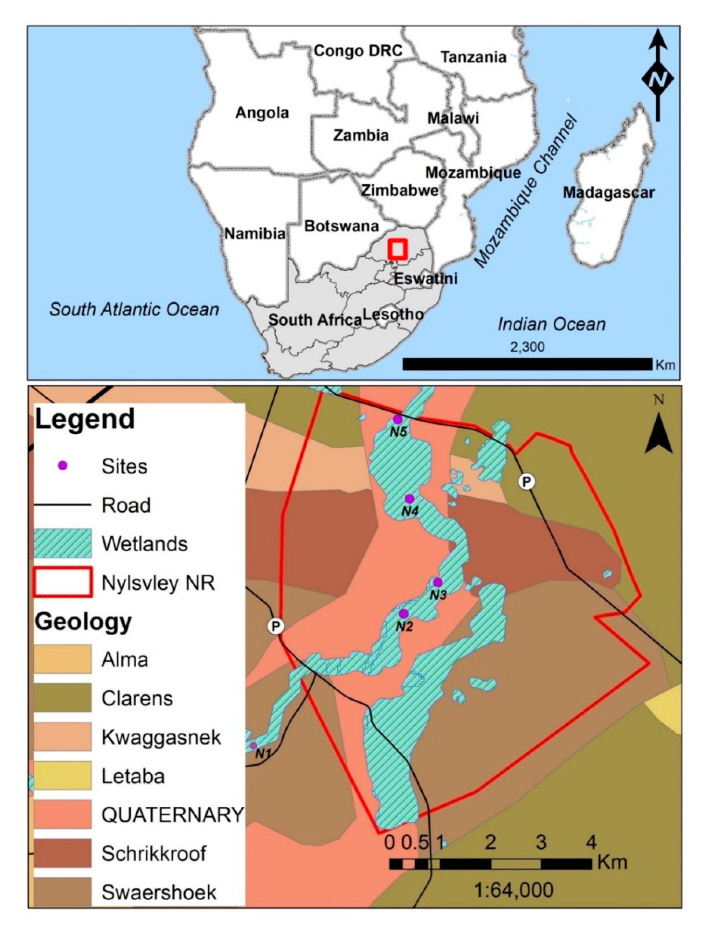
2.1. Study Area

The Nylsvley wetland (24°39′17″ S, 28°41′28″ E) is formed along a section of the Nyl River and is situated in the Waterberg region, Limpopo Province of South Africa between 1080 and 1155 m above sea level. The area was declared a Ramsar wetland site of international conservation significance in 1997. The wetland is made up of extensive reed beds and grass veld, surrounded by open savanna woodlands [46]. Nylsvley receives approximately 620 mm of rainfall per annum, with dry and rainy seasons occurring between April and September, and October and March, respectively. Average temperatures during the day range from 20.5 °C in June to 28.9 °C in midsummer, and temperature drops to below zero in winter, especially during the night, and can exceed 39 °C in summer. Potential sources of pollution/contamination include upstream anthropogenic activities, particularly within the town of Modimolle (i.e., 35 km from Nylsvley Wetland) and the surrounding agricultural farms [47]. The present study was carried out in five randomly selected upper reach sites (i.e., outside reserve (N1), Nylsvley Nature Reserve (N2, N3, N4, N5)) of the Nylsvley Wetland in September 2018 (Figure 1). Site N1 was situated on the narrow (width ≈50 m) upper reaches of the Nylsvley Wetland and site N5 had the largest width (>300 m) of the wetland area sampled. Phragmites australis, Persicaria spp., and Ludwigia spp. dominated the macrophytes across all sites, with only a small area being covered by Phragmites australis at site N5.

2.2. Sediment Collection and Processing

Integrated sediment samples (1.5 kg; N = 2 replicate cores × 5 sites × 6 depth ranges per core) were collected using a hand auger, after the removal of the overlaying debris, within the permanent zone (i.e., main stem) of each site along varying soil depth ranges: 0–20 cm, 20–40 cm, 40–60 cm, 60–80 cm, 80–100 cm, and 120–140 cm, respectively. For background values, samples (n = 5) were collected randomly from a nearby forest area that was relatively pristine with no known past or present anthropogenic impacts. The samples were then placed separately in clean polyethylene ziplock bags. Sampled sediments were transported to the laboratory (University of Venda, Department of Ecology and Resource Management) and oven dried at 60 °C for 48–72 h, before being disaggregated in a porcelain mortar and sieved to remove unwanted plant roots and debris through sieving (mesh size 0.05 mm).

2.3. Sediment Analysis

Detailed methods for cation, metal, and nutrients are presented in Dalu et al. [48], a paper from the same project. The examined metals were selected based on previous studies that have been carried out on the river system [26,39]. In brief, for each profile, alkali and alkaline earth metals (i.e., Ca, K, Na, Mg) as well as other metal cations (i.e., B, Cu, Fe, Mn, Zn) were measured using an Inductively coupled plasma atomic emission spectroscopy instrument (see Clesceri et al. [49] for detailed methodology), while the total nitrogen and phosphorus were analyzed using a SEAL AutoAnalyzer 3 high resolution and Bray-2 extract as described by Bray and Kurtz [50] and AgriLASA [51]. To estimate the accuracy of this method, a natural standard-certified reference soil, namely SARM-51 (MINTEK) and SL-1 (IAEA), digested and analyzed in triplicate, was used for recovery tests. The percentage recoveries of the certified values ranged between 89% and 109% for all metals.

2.4. Data Analysis

All data were assessed for normality and homogeneity of variance and were found to conform to parametric assumptions. Differences in metal and nutrient concentrations among sites (i.e., N1–N5) and with sediment depth (i.e., 0–20 cm, 20–40 cm, 40–60 cm, 60–80 cm, 80–100 cm and 120–140 cm) were, therefore, analyzed using two-way ANOVA tests in SPSS version 16 [52]. Where significant differences were observed, Tukey’s post hoc analyses were conducted to assess pairwise comparisons for the different study sites and sediment depths.
To effectively ascertain the extent of metal pollution within the Nylsvley Wetland, selected metal concentrations were compared with international standards of sediment quality guidelines (SQGs). These values can be considered as threshold concentrations for metals that cause adverse biological effects in an aquatic environment. The Canadian sediment quality guidelines [53], which comprise two levels, i.e., the low effect level (LEL) and severe effect level (SEL), were utilized here, and they are the mostly commonly used, as South Africa and the region at large do not have sediment quality guidelines.
The following were calculated for the Nylsvley Wetland: the geoaccumulation index (Igeo), which assesses individual heavy metal pollution levels in sediment [54]; the enrichment factor (EF), which is a measure of concentration of a certain metal in the sediment relative to its natural background concentration [55]; and the pollution load index (PLI), which measures the degree of contamination of the soil by metals [56]. The Fe concentration sample was utilized as the level of a predetermined reference metal as per a previous study by Dahms et al. [26] in the Nyl River. Iron (Fe) was chosen as the reference metal as its distribution in an aquatic ecosystem is unrelated to other metals [57]. The description of each sediment metal index is highlighted in Table 1.
A principal component analysis (PCA) with the varimax rotation method was used to determine the natural and anthropogenic sources of sediment metals across depths and sites in PC-ORD version 5.10 [58]. A two-way cluster analysis, using Ward’s average group linkage method and correlation as a distance measure, was used for metal source identification. Furthermore, using a Pearson correlation, we tested for relationships between metals and nutrient concentrations using SPSS version 16 [52].

3. Results

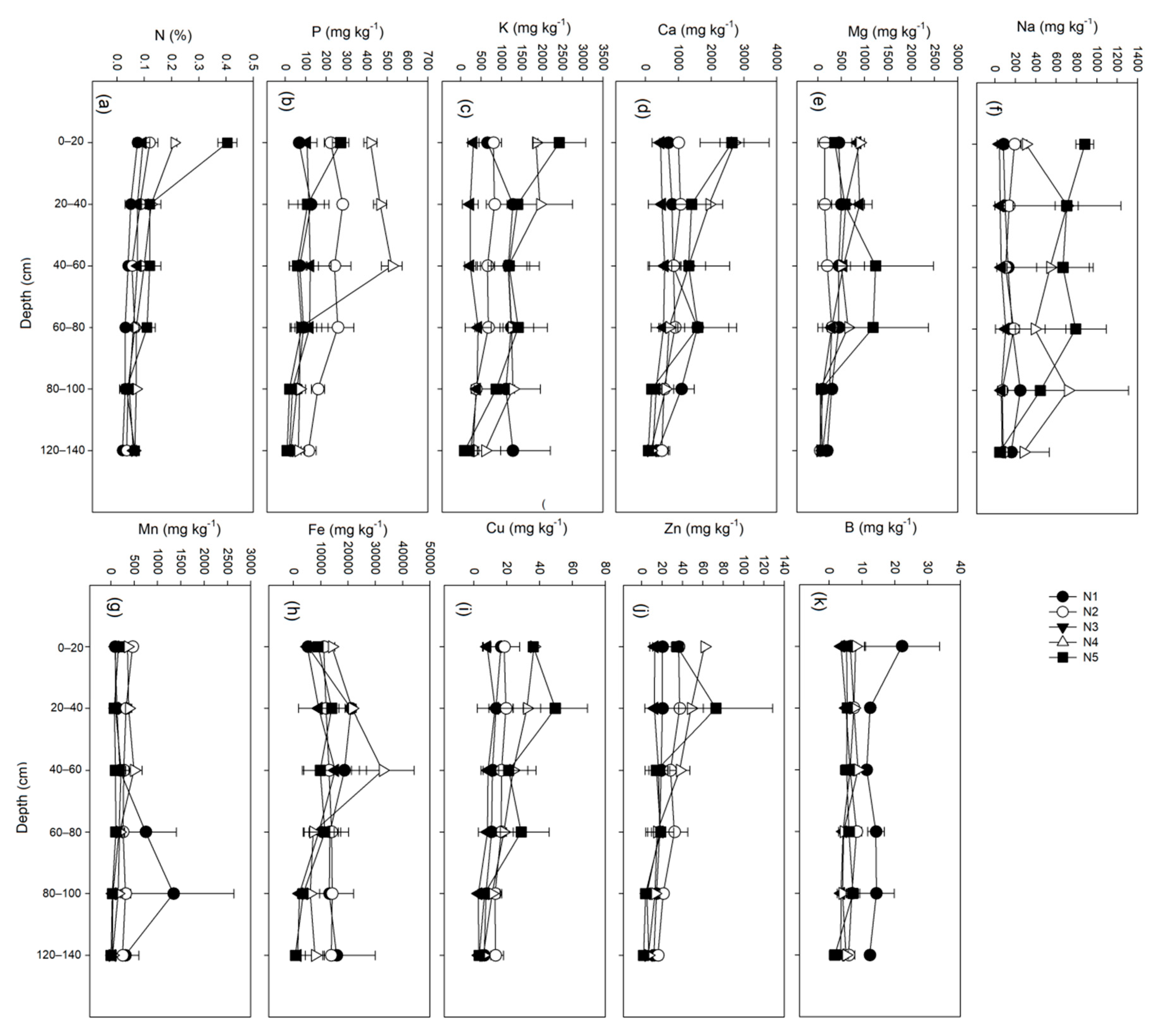
3.1. Metal and Nutrient Vertical Distribution Profiles

The vertical distributions of nutrients and metals along soil profiles at the five sampling sites are highlighted in Figure 2. Significant differences in nutrient (i.e., N, P) and metal (i.e., K, Mg, Na, Fe, Cu, B) concentrations were found (p < 0.05) across study sites, whereas nutrients (i.e., N, P) and metals (i.e., Ca, Mg, Fe, Cu, Zn) were significantly different (p < 0.05) with sediment depths (Table 2). The overall mean nutrient and metal concentration decreased as the soil depth increased. Pairwise post hoc comparisons are presented in Table S1; for Fe across study sites and sediment depths, pairwise similarities (p > 0.05) were observed.

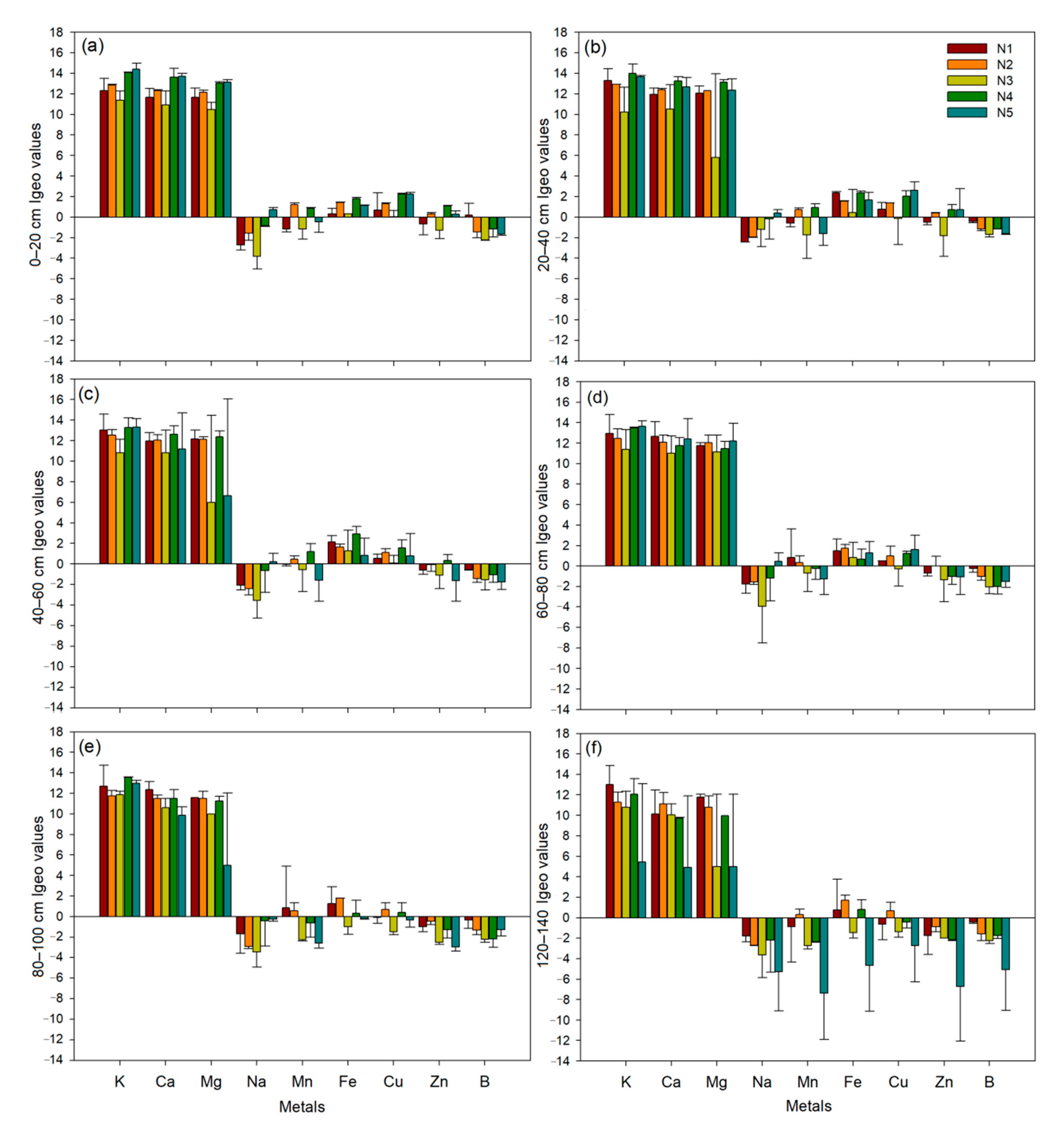
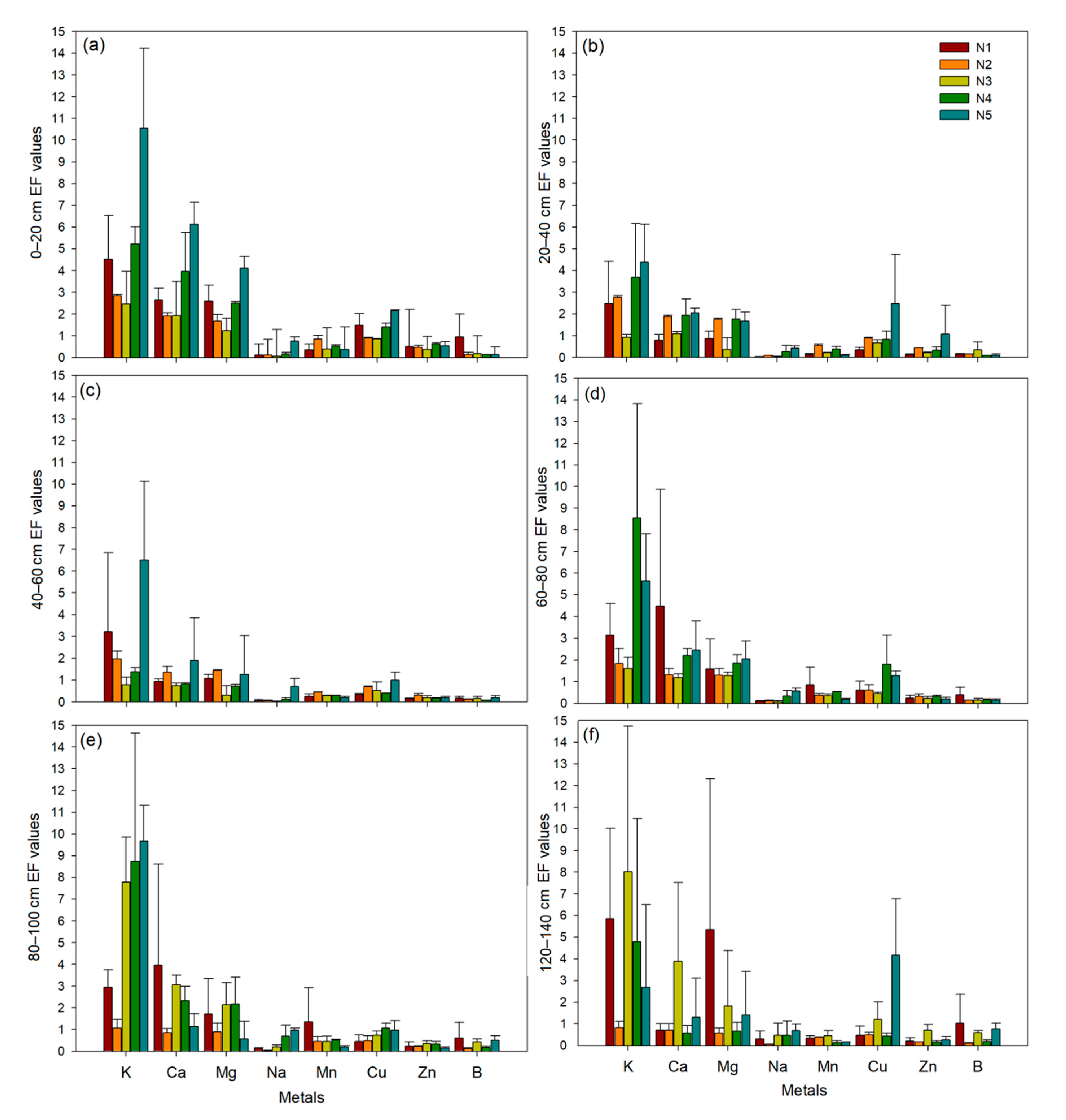
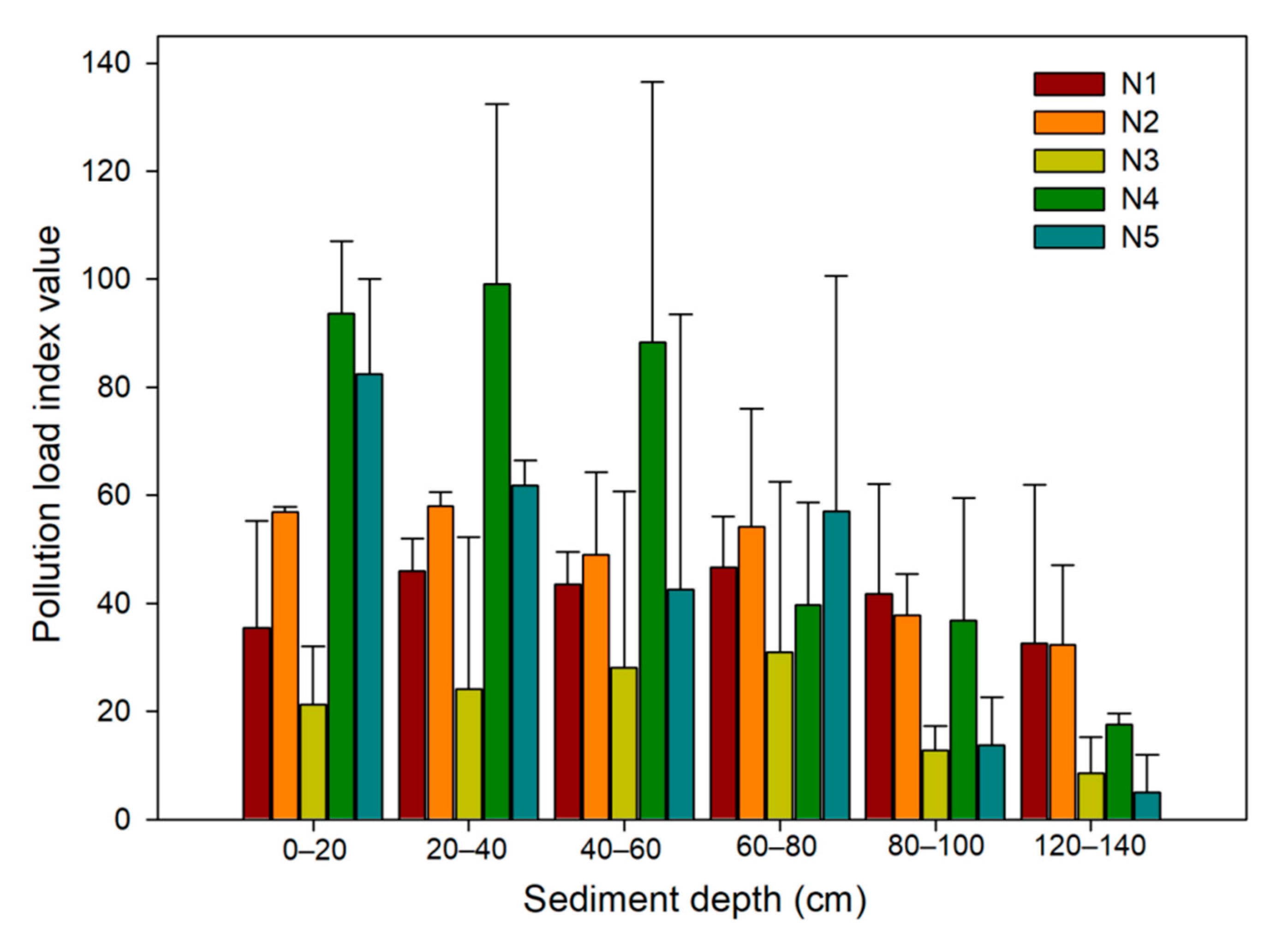
3.2. Sediment Quality Guidelines

When compared against international standards, most of the assessed metals were within the “no effect” level across the different sites and depths, except for a few sites/depths presented in Table S2. For Mn, sites N1 (depth 60–80 cm), N2 (depth 0–20 cm), and N4 (depth 40–60 cm) were within the LEL threshold, whereas site N1 (depth 80–100 cm) was in the SEL level (Table S2). Considering Fe concentrations, 2 sites (N1, N4) and two depths (20–40 cm; 40–60 cm) were in the LEL range, whereas Cu concentration were within the LEL level for sites N1 (depth 0–20 cm), N2 (depths 0–80 cm), N4 (depths 0–80 cm), and N5 (depths 0–80 cm) (Table S2). All Zn concentration for all sites and depths were within the no effect level.
The K, Ca, and Mg concentration showed extreme contamination across all sites and depths (Figure 3). The Na and B Igeo values were grouped into class 0, indicative of no contamination for most study sites and sediment depths, with a few sediment depths in different study sites indicating class 1 (no to moderate contamination). For Mn, Fe, Cu, and Zn, the Igeo values ranged mostly from class 0 (no contamination) to class 3 (moderate to strong contamination) (Figure 3). We found significant differences (p < 0.05) across study sites for K, Mg, Na, Mn, Cu, and B concentrations, and sediment depths for Ca, Mg, Fe, Cu, and Zn concentrations (Table 2). Using Tukey’s post hoc analyses, significant differences were observed for study site pairwise combinations for Mg, Mn, Fe, and Cu, and sediment depth for Ca, Mg, Fe, Cu, Zn for selected sites and depths (see Table S3).
The EF values for K, Ca, and Mg showed extremely high enrichment levels for all sites and sediment depths (Figure 4). The Na, Mn, Fe, Cu, Zn, and B concentration showed mostly background enrichment levels. The exceptions were Mn at site N1 (depth 80–100 cm), Cu (site N3, depth 120–140 cm; N4, depth 0–20 cm, 60–100 cm; N5, 40–100 cm), Na (site N5, depth 80–100 cm) and Zn (site N5, depth 20–40 cm) which showed low enrichment, and Cu (site N5, depth 0–40 cm) which had moderate enrichment (Figure 4). Using two-way ANOVAs, significant differences (p < 0.05) were observed across study sites for K, Na, Cu, and B concentrations, and also in sediment depths for K and Na concentrations (Table 2). Using Tukey’s post hoc analyses, nonsignificant differences (p > 0.05) were observed for all metals across the different sediment depths, whereas significant site differences (p < 0.05) were observed for K, Na, Cu, and B (see Table S3).
Most of the sediments across the different sites and sediment depths indicated deterioration of sediment quality (Figure 5). The indicated deterioration of sediment quality decreased with sediment depth and was generally highest for sites N4 and N5 (depths 0–60 cm). The pollution load index values were significantly different among study sites (F = 5.275, p = 0.002) and sediment depths (F = 4.999, p = 0.002). Using Tukey’s post hoc analysis, significant differences in PLI values were observed for sites N2 vs. N3 (p = 0.046) and N3 vs. N4 (p < 0.001), and sediment depth of 0–20 cm vs. 120–140 cm (p = 0.007), 20–40 cm vs. 120–140 cm (p = 0.008), 40–60 cm vs. 120–140 cm (p = 0.046), and 20–40 cm vs. 80–100 cm (p = 0.008).

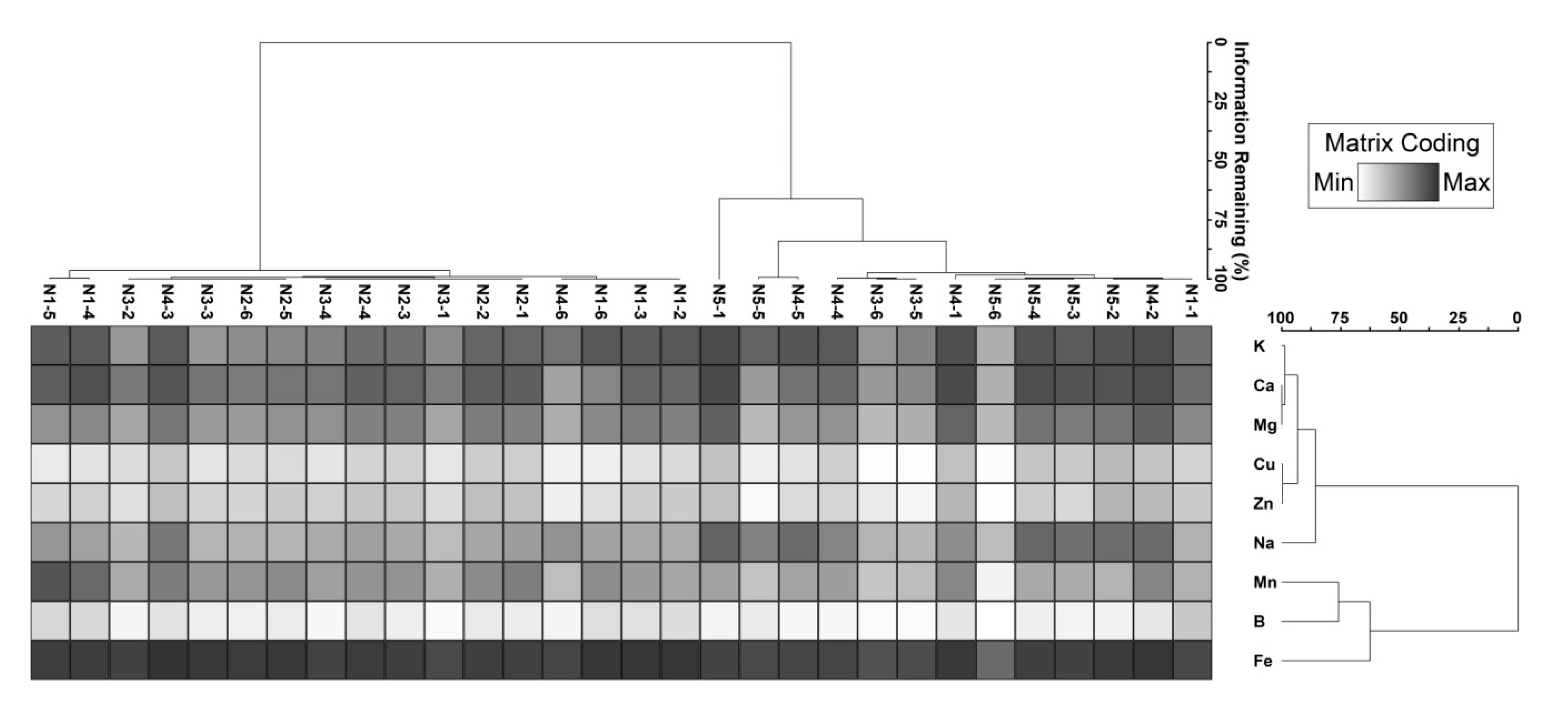
3.3. Assessing the Relationship Between the Measured Metal Variables

Pearson correlations highlighted that most wetland sediment metals and nutrients were significantly correlated with each other, indicating a strong positive association, except for Mn and B, which were only correlated with a few of the metals and nutrients (Table 3). The Mn was significantly positively correlated with K alone, whereas B was significantly positively correlated with Ca, Mg, and Fe (Table 3).
The PCA ordination technique showed that the first two principal components (PC) explained 74.7% of the total variance, with PC1 and PC2 explaining 55.7% and 19.0% of the variance, respectively (Table 4). The principal component analysis classified metals into two groups, with group 1 consisting of all metals, except for Mn and B, which were the only metals in group 2 (Table 4). The two-way cluster analysis results identified 2 distinct groups: Group 1 consisted of Mn, B, and Fe and was clearly distinguishable from group 2 (i.e., K, Ca, Mg, Na, Cu, Zn; Figure 6). For sediment depth, the cluster analysis identified two groups. Group 1 consisted of sediment depths in sites N4 (all depths except 40–60 cm, 120–140 cm), N5 (all depths), N1 (0–20 cm), and N3 (80–100 cm, 120–140 cm). Group 2 consisted of sediment depths in sites N1 (all depths excluding 0–20 cm), N2 (all depths), N3 (all depths excluding 80–100 cm, 120–140 cm), and N4 (40–60 cm, 120–140 cm) (Figure 6).

4. Discussion

The results obtained in our study highlight that metal concentrations were elevated in surface sediment, in contrast to our first hypothesis. Furthermore, we observed that lower reach sites were generally more polluted compared to the upper reach sites (Figure 2). Upstream land use activities have previously been identified as drivers of metals within this system by Greenfield et al. [39] and Dahms et al. [26], who quantified the accumulation of metals within the Nyl River. Prusty et al. [60], Bai et al. [13], and Zhang et al. [61] highlighted that Cu and Zn tended to decrease with increasing soil depths in wetland ecosystems, similar to findings in the present study. Our observations were also similar to Zhang et al. [44], who found that the vertical distribution of metals (e.g., As, Cu, Pb) was greater at the surface than those in the subsurface layer. The increase in metal concentrations in a downstream direction may have been a result of hydrological dynamics, and in particular, water velocity. As water velocity decreases are associated with lower metal suspension potential, water moving the confined river banks of the Nyl River onto the more open shallow wetland areas likely resulted in increased metal deposition onto sediments. Vegetation likely played a role in spatial metal concentration dynamics [62], although this was not assessed in the present study.
The sediment vertical distribution results based on the international guidelines showed that the surface to midsurface sediments (depth 0–80 cm) were mostly contaminated when compared to subsurface soils (depth 120–140cm). However, the sediment quality was generally within the acceptable level as per the Canadian sediment quality guidelines [53]. This was particularly the case for Mn, Fe, and Zn, where only a few sites and depths exceeded the “no effect” level, whilst Cu levels were most consistently elevated at shallow depths. Nonetheless, those sites that exceeded standards have been identified for further monitoring effort. These differences were probably influenced by variations in metal settling ability, as well as differences in affinity ability as sediments aggregate and textures differ with depth and sites. Wepener and Vermeulen [63] highlighted that sediment particle size influences the spatial variation of metals, and this was observed in our study, as the polluted surface sediments were mostly clays, and the subsurface sediments were mostly silt and sand (T. Dalu, personal observation). Acosta et al. [64] also highlighted that the duration and timing of flood events will result in the uneven distribution of metals across sites and sediment depths. Furthermore, these hydrological condition differences would affect soil physicochemical properties, such as salinity, which would additionally alter metal mobility in sediments [65]. For example, Greenfield [39] and Dahms et al. [26] observed that Fe, Zn, and Mn concentrations exceeded the sediment quality guidelines (i.e., LEL) for the surface sediments in Nylsvley Wetland, yet they found that these concentration levels were mostly within the permissible limits, which implies that the wetland was effectively removing these metals or they were being taken up by the abundant plant community.
Overall, the study results demonstrated a high degree of metal pollution in the wetland sediment across sites and sediment depths, as evidenced by the high Igeo and EF (for K, Ca, and Mg) and PLI values, but a relatively low degree of metal pollution for Na, Fe, Cu, B, Mn, and Zn. We speculate that the high metal loads for K, Ca, and Mg in relation to the background values reflect the increased urbanization and agricultural activities upstream in the headwaters of the Nyl River, similarly to a study by Xiao et al. [66]. It is also important to note that increased K, Ca, and Mg enrichment can alter other wetland biogeochemical processes, such as causing nutrient imbalances and increased salinity, thereby endangering the fragile ecosystem. These high metal concentrations particularly for Cu, Fe, and Mn alone might have adverse ecological implications for benthic fauna and flora. However, the potential risk that metal concentrations in the sediments pose does not solely depend on total concentrations but also on the bioavailable fractions determination [17,67].
Multivariate analyses (i.e., PCA, cluster analysis) are some of the most widely applied in the source identification of metals, as they provide information on metal association in areas of interest [33,44,68,69]. Pandey et al. [70] highlighted that a two-way cluster analysis classifies the variables into different clusters depending upon the resemblance among them. A high correlation among the different metals is therefore often indicative of a common source and mutual dependence [44,68]. Thus, the Pearson correlations reported in the present study suggest that most metals might have originated from a similar source to that of Mn and B, owing to a lack of significant differences. The PCA and cluster analyses further highlighted that the observed metal concentration differences could be highly site-specific, linked to additional factors such as anthropogenic point sources and local bedrock. The two-way cluster analysis additionally found that there were differences in the site and sediment depth metal variations with a strong separation between the upper reach sites (i.e., N1–N3) and lower reach sites (i.e., N4–N5). The differences could be attributed to differences in wetland width, which might cause metal deposition and accumulation variations as indicated by high concentrations at downstream sites N4 and N5 (Figure 2).

5. Conclusions

Overall, K, Ca, and Mg concentrations should be carefully monitored within the area to avoid potential ecotoxicity to the wildlife in Nylsvley Wetland, based on the geoaccumulation indices and enrichment factors. These results provide baseline information for the Nylsvley Wetland in relation to sediment metal pollution; however, further studies are required to fully understand metal dynamics within the system. The specific sources of metal contaminants also require further elucidation to further inform management efforts. Gregorauskiene and Kadunas [71] highlighted that localized sediment metal concentration might be associated with plant cycling, which leads to the movement of metals. In such cases, assessments of wetland plant contributions to metals’ vertical distribution dynamics in the sediment would also be useful. In addition, further investigations into the seasonal variability in the sediment and water quality across the wetland zones are needed to understand the metal dynamics within the sediment and water interface.

Supplementary Materials

The following are available online at https://www.mdpi.com/2073-4441/12/10/2779/s1, Table S1. Tukey’s pairwise comparisons results for the significant (p < 0.05) metal and nutrient concentration variables. Table S2. Sediment quality guidelines for mean Mn, Fe, Cu, and Zn concentrations (mg kg−1) for different sediment depths across study sites. Table S3. Tukey’s pairwise comparisons results for the significant (p < 0.05) sediment quality guideline variables

Author Contributions

Conceptualization, T.D. and R.J.W.; Methodology, T.D., F.M.M., R.T. and R.J.W.; Formal Analysis, T.D., R.T. and R.N.C.; Investigation, T.D., F.M.M., R.T and R.J.W.; Resources, T.D.; Data Curation, T.D. and R.T.; Writing—Original Draft Preparation, T.D., R.T. and R.N.C.; Writing—Review and Editing, T.D., R.T., R.N.C., F.M.M. and R.J.W.; Visualization, T.D., R.J.W. and R.N.C.; Supervision, R.J.W., F.M.M. and T.D.; Funding Acquisition, T.D. All authors have read and agreed to the published version of the manuscript.

Funding

The study was funded by the University of Venda Niche Grant (SES/18/ERM/10) and the NRF Thuthuka Grant (117700). R.C. and R.J.W. acknowledge funding from the Alexander von Humboldt Foundation and Botswana International University of Science and Technology, respectively.

Acknowledgments

Thendo Mutshekwa is thanked for helping with the field work and Farai Dondofema for making Figure 1.

Conflicts of Interest

The authors declare no conflict of interest.

References

  1. Cherry, J.A. Ecology of Wetland Ecosystems: Water, Substrate, and Life. Nat. Educ. Knowl. 2011, 3, 16. [Google Scholar]
  2. Dalu, T.; Wasserman, R.J.; Dalu, M.T.B. Agricultural intensification and drought frequency increases may have landscape-level consequences for ephemeral ecosystems. Glob. Chang. Biol. 2017, 23, 983–985. [Google Scholar] [CrossRef] [PubMed]
  3. Bai, J.; Zhao, Q.; Wang, W.; Wang, X.; Jia, J.; Cui, B.; Liu, X. Arsenic and heavy metals pollution along a salinity gradient in drained coastal wetland soils: Depth distributions, sources and toxic risks. Ecol. Indic. 2019, 96, 91–98. [Google Scholar] [CrossRef]
  4. Bird, M.S.; Mlambo, M.C.; Wasserman, R.J.; Dalu, T.; Holland, A.J.; Day, J.A.; Villet, M.H.; Bilton, D.T.; Barber-James, H.M.; Brendonck, L. Deeper knowledge of shallow waters: Reviewing the invertebrate fauna of southern African temporary wetlands. Hydrobiologia 2019, 827, 89–121. [Google Scholar] [CrossRef]
  5. Astle, J.H.; Boss, J. Your wetlands are not a wasteland: Developing natural areas for program use. Camping Mag. 2000, 73, 34–37. [Google Scholar]
  6. Tennant-Wood, R. From wasteland to wetland: Creating a community ecological resource from waste water in regional New South Wales. Local Environ. 2004, 9, 527–539. [Google Scholar] [CrossRef]
  7. Reddy, K.R.; DeLaune, R.D. Biogeochemistry of Wetlands: Science and Application; CRC Press: Boca Raton, FL, USA, 2008. [Google Scholar]
  8. Zhao, Q.; Bai, J.; Huang, L.; Gu, B.; Lu, Q.; Gao, Z. A review of methodologies and success indicators for coastal wetland restoration. Ecol. Indic. 2016, 60, 442–452. [Google Scholar] [CrossRef]
  9. Cui, B.; He, Q.; Gu, B.; Bai, J.; Liu, X. China’s coastal wetlands: Understanding environmental changes and human impacts for management and conservation. Wetlands 2016, 36, 1–9. [Google Scholar] [CrossRef] [Green Version]
  10. Cuthbert, R.N.; Weyl, O.L.F.; Wasserman, R.J.; Dick, J.T.; Froneman, P.W.; Callaghan, A.; Dalu, T. Combined impacts of warming and salinisation on trophic interactions and mortality of a specialist ephemeral wetland predator. Freshw. Biol. 2019, 64, 1584–1592. [Google Scholar] [CrossRef]
  11. Chen, H.; Zhang, W.; Gao, H.; Nie, N. Climate change and anthropogenic impacts on wetland and agriculture in the Songnen and Sanjiang Plain, Northeast China. Remote Sens. 2018, 10, 356. [Google Scholar] [CrossRef] [Green Version]
  12. Gopal, B. Perspectives on wetland science, application and policy. Hydrobiologia 2003, 490, 1–10. [Google Scholar] [CrossRef]
  13. Bai, J.; Xiao, R.; Zhao, Q.; Lu, Q.; Wang, J.; Reddy, K.R. Seasonal dynamics of heavy elements in tidal salt marsh soils as affected by the flow-sediment regulation regime. PLoS ONE 2014, 9, e107738. [Google Scholar] [CrossRef] [PubMed]
  14. Khaledian, Y.; Pereira, P.; Brevik, E.C.; Pundyte, N.; Paliulis, D. The influence of organic carbon and pH on heavy metals, potassium, and magnesium levels in Lithuanian Podzols. Land Degrad. Dev. 2017, 28, 345–354. [Google Scholar] [CrossRef]
  15. Leroy, M.C.; Marcotte, S.; Legras, M.; Moncond’huy, V.; Le Derf, F.; Portet-Koltalo, F. Influence of the vegetative cover on the fate of trace metals in retention systems simulating roadside infiltration swales. Sci. Total Environ. 2017, 580, 482–490. [Google Scholar] [CrossRef]
  16. De Paula Filho, F.J.; Marins, R.V.; de Lacerda, L.D.; Aguiar, J.E.; Peres, T.F. Background values for evaluation of heavy metal contamination in sediments in the Parnaíba River Delta estuary, NE Brazil. Mar. Pollut. Bull. 2015, 91, 424–428. [Google Scholar] [CrossRef] [PubMed]
  17. Bere, T.; Dalu, T.; Mwedzi, T. Detecting the impact of heavy metal contaminated sediment on benthic macroinvertebrate communities in tropical streams. Sci. Total Environ. 2016, 572, 147–156. [Google Scholar] [CrossRef] [PubMed]
  18. Dalu, T.; Wasserman, R.J.; Tonkin, J.D.; Mwedzi, T.; Magoro, M.L.; Weyl, O.L.F. Water or sediment? Partitioning the role of water column and sediment chemistry as drivers of macroinvertebrate communities in an austral South African stream. Sci. Total Environ. 2017, 607, 317–325. [Google Scholar] [CrossRef]
  19. Pal, S.; Chattopadhyay, B.; Datta, S.; Mukhopadhyay, S.K. Potential of wetland macrophytes to sequester carbon and assessment of seasonal carbon input into the East Kolkata Wetland Ecosystem. Wetlands 2017, 37, 497–512. [Google Scholar] [CrossRef]
  20. Pal, S.; Chakraborty, S.; Datta, S.; Mukhopadhyay, S.K. Spatio-temporal variations in total carbon content in contaminated surface waters at East Kolkata Wetland Ecosystem, a Ramsar Site. Ecol. Eng. 2018, 110, 146–157. [Google Scholar] [CrossRef]
  21. Pejman, A.; Bidhendi, G.N.; Ardestani, M.; Saeedi, M.; Baghvand, R. A new index for assessing heavy metals contamination in sediments: A case study. Ecol. Indic. 2015, 58, 365–373. [Google Scholar] [CrossRef]
  22. Kifayatullah, K.; Lu, Y.; Khan, H.; Zakir, S.; Ihsanullah, J.; Khan, S. Health risk associated with heavy metal in the drinking water of Swat, northern Pakistan. J. Environ. Sci. 2013, 25, 2003–2013. [Google Scholar]
  23. Clark, J.H.A.; Tredoux, M.; van Huyssteen, C.W. Heavy metals in the soils of Bloemfontein, South Africa: Concentration levels and possible sources. Environ. Monit. Assess. 2015, 187, 439–449. [Google Scholar] [CrossRef] [PubMed]
  24. Ramachandra, T.V.; Sudarshan, P.B.; Mahesh, M.K.; Vinay, S. Spatial patterns of heavy metal accumulation in sediments and macrophytes of Bellandur wetland, Bangalore. J. Environ. Manag. 2018, 206, 1204–1210. [Google Scholar] [CrossRef]
  25. Greenfield, R.; van Vuren, J.H.J.; Wepener, V. Determination of sediment quality in the Nyl River system, Limpopo province, South Africa. Water SA 2007, 33, 693–700. [Google Scholar] [CrossRef] [Green Version]
  26. Dahms, S.; Baker, N.J.; Greenfield, R. Ecological risk assessment of trace elements in sediment: A case study from Limpopo, South Africa. Ecotoxicol. Environ. Saf. 2017, 135, 106–114. [Google Scholar] [CrossRef]
  27. Binda, G.; Pozzi, A.; Livio, F. An integrated interdisciplinary approach to evaluate potentially toxic element sources in a mountainous watershed. Environ. Geochem. Health 2019, 42, 1255–1272. [Google Scholar] [CrossRef]
  28. Dalu, T.; Wasserman, R.J.; Magoro, M.L.; Froneman, P.W.; Weyl, O.L.F. River nutrient water and sediment measurements inform on nutrient retention, with implications for eutrophication. Sci. Total Environ. 2019, 684, 296–302. [Google Scholar] [CrossRef]
  29. Vu, C.T.; Lin, C.; Shern, C.C.; Yeh, G.; Tran, H.T. Contamination, ecological risk and source apportionment of heavy metals in sediments and water of a contaminated river in Taiwan. Ecol. Indic. 2017, 82, 32–42. [Google Scholar] [CrossRef]
  30. Wall, F.; Rollat, A.; Pell, R.S. Responsible sourcing of critical metals. Elements 2017, 13, 313–318. [Google Scholar] [CrossRef] [Green Version]
  31. Wang, S.; Wang, W.; Chen, J.; Zhao, L.; Zhang, B.; Jiang, X. Geochemical baseline establishment and pollution source determination of heavy metals in lake sediments: A case study in Lihu Lake, China. Sci. Total Environ. 2019, 657, 978–986. [Google Scholar] [CrossRef]
  32. Bai, J.; Xiao, R.; Cui, B.; Zhang, K.; Wang, Q.; Liu, X.; Gao, H.; Huang, L. Assessment of heavy metal pollution in wetland soils from the young and old reclaimed regions in the Pearl River Estuary, South China. Environ. Pollut. 2011, 59, 817–824. [Google Scholar] [CrossRef] [PubMed]
  33. Dalu, T.; Wasserman, R.J.; Wu, Q.; Froneman, W.P.; Weyl, O.L.F. River sediment metal and nutrient variations along an urban–agriculture gradient in an arid austral landscape: Implications for environmental health. Environ. Sci. Pollut. Res. 2018, 25, 2842–2852. [Google Scholar] [CrossRef] [PubMed]
  34. Förstner, U.; Wittmann, G.T. Metal Pollution in the Aquatic Environment; Springer Science and Business Media: Berlin, Germany, 2012. [Google Scholar]
  35. Chattopadhyay, B.; Chatterjee, A.; Mukhopadhyay, S.K. Bioaccumulation of metals in the East Calcutta wetland ecosystem. Aquat. Ecosyst. Health Manag. 2002, 5, 191–203. [Google Scholar] [CrossRef]
  36. Lau, S.S.S.; Chu, L.M. The significance of sediment contamination in a coastal wetland, Hong Kong, China. Water Res. 2000, 34, 379–386. [Google Scholar] [CrossRef]
  37. Chatterjee, S.; Chetia, M.; Singh, L.; Chattopadhyay, B.; Datta, S.; Mukhopadhyay, S.K. A study on the phytoaccumulation of waste elements in wetland plants of a Ramsar site in India. Environ. Monit. Assess. 2011, 178, 361–371. [Google Scholar] [CrossRef]
  38. Zhang, M.; Cui, L.; Sheng, L.; Wang, Y. Distribution and enrichment of heavy metals among sediments, water body and plants in Hengshuihu Wetland of Northern China. Ecol. Eng. 2009, 35, 563–569. [Google Scholar] [CrossRef]
  39. Greenfield, R.; van Vuren, J.H.J.; Wepener, V. Heavy metal concentrations in the water of the Nyl river system, South Africa. Afr. J. Aquat. Sci. 2012, 37, 219–224. [Google Scholar] [CrossRef]
  40. Wang, X.C.; Feng, H.; Ma, H.Q. Assessment of metal contamination in surface sediments of Jiaozhou Bay, Qingdao, China. Clean Soil Air Water 2007, 35, 62–70. [Google Scholar] [CrossRef]
  41. Akele, M.L.; Kelderman, P.; Koning, C.W.; Irvine, K. Heavy metal distributions in the sediments of the Little Akaki River, Addis Ababa. Ethiopia. Environ. Monit. Assess. 2016, 188, 1–13. [Google Scholar] [CrossRef]
  42. Coxon, T.M.; Odhiambo, B.K.; Giancarlo, L.C. The impact of urban expansion and agricultural legacies on trace metal accumulation in fluvial and lacustrine sediments of the lower Chesapeake Bay basin, USA. Sci. Total Environ. 2016, 568, 402–414. [Google Scholar] [CrossRef]
  43. Bellasi, A.; Binda, G.; Pozzi, A.; Galafassi, S.; Volta, P.; Bettinetti, R. Microplastic Contamination in Freshwater Environments: A Review, Focusing on Interactions with Sediments and Benthic Organisms. Environments 2020, 7, 30. [Google Scholar] [CrossRef] [Green Version]
  44. Zhang, G.; Bai, J.; Zhao, Q.; Jia, J.; Wen, X. Heavy metals pollution in soil profiles from seasonal-flooding riparian wetlands in a Chinese delta: Levels, distributions and toxic risks. Phys. Chem. Earth ABC 2017, 97, 54–61. [Google Scholar] [CrossRef] [Green Version]
  45. Tshimomola, T. The population biology of Sclerocarya birrea at Nylsvley Nature Reserve, Limpopo Province, South Africa. Ph.D. Thesis, University of Venda, Thohoyandou, South Africa, 2017. [Google Scholar]
  46. Walker, B.H. The Savannas: Biogeography and Geobotany. J. Ecol. 1987, 24, 1082–1083. [Google Scholar] [CrossRef]
  47. Baker, N.J.; Greenfield, R. Shift happens: Changes to diversity of riverine aquatic macroinvertebrate communities in response to sewage effluent runoff. Ecol. Indic. 2019, 102, 813–821. [Google Scholar] [CrossRef]
  48. Dalu, T.; Murudi, T.T.; Dondofema, F.; Wasserman, R.J.; Chari, L.D.; Murungweni, F.M.; Cuthbert, R.N. Balloon milkweed Gomphocarpus physocarpus distribution and drivers in an internationally protected wetland. Bioinvasions Rec. 2020, 9, 627–641. [Google Scholar] [CrossRef]
  49. Clesceri, L.S.; Greenberg, A.E.; Eaton, A.D. Standard Methods for the Examination of Water and Wastewater, 20th ed.; American Public Health Association: Washington, DC, USA, 1998. [Google Scholar]
  50. Bray, R.H.; Kurtz, L.T. Determination of total, organic, and available forms of phosphorus in soils. Soil Sci. 1945, 59, 39–45. [Google Scholar] [CrossRef]
  51. Agri Laboratory Association of Southern Africa (AgriLASA). Soil Handbook; Agri Laboratory Association of Southern Africa: Pretoria, South Africa, 2004. [Google Scholar]
  52. SPSS Inc. SPSS Release 16.0.0 for Windows; Polar Engineering and Consulting; SPSS Inc.: Chicago, IL, USA, 2007. [Google Scholar]
  53. Persaud, D.; Jaagumagi, R.; Hayton, A. Guidelines for the Protection and Management of Aquatic Sediment. Quality in Ontario; Ministry of the Environment and Energy: Sudbury, ON, Canada, 1993. [Google Scholar]
  54. Muller, G. Index of geoaccumulation in sediments of the Rhine River. J. Geol. 1969, 2, 108–118. [Google Scholar]
  55. Buat-Menard, P.; Chesselet, R. Variable influence of atmospheric flux on the heavy metal chemistry of oceanic suspended matter. Earth Planet. Sci. Lett. 1979, 42, 398–411. [Google Scholar] [CrossRef]
  56. Tomlinson, D.L.; Wilson, J.G.; Harris, C.R.; Jeffrey, D.W. Problems in the assessment of heavy-metal levels in estuaries and the formation of a pollution index. Helgol. Meeresunters. 1980, 33, 566–575. [Google Scholar] [CrossRef] [Green Version]
  57. Abrahim, G.M.S.; Parker, R.J. Assessment of heavy metal enrichment factors and the degree of contamination in marine sediments from Tamaki Estuary, Auckland, New Zealand. Environ. Monit. Assess. 2008, 136, 227–238. [Google Scholar] [CrossRef]
  58. McCune, B.; Grace, J.B. Analysis of Ecological Communities; MjM Software: Gleneden Beach, OR, USA, 2002. [Google Scholar]
  59. Sutherland, R.A. Bed sediment-associated heavy metals in an urban stream, Oahu, Hawaii. Environ. Geol. 2000, 39, 611–627. [Google Scholar] [CrossRef]
  60. Prusty, B.; Kumar, A.; Azeez, P.A. Vertical distribution of alkali and alkaline earth metals in the soil profile of a wetland-terrestrial ecosystem complex in India. Austal. J. Soil Res. 2007, 5, 533–542. [Google Scholar] [CrossRef]
  61. Zhang, Z.; Zheng, D.; Xue, Z.; Wu, H.; Jiang, M. Identification of anthropogenic contributions to heavy metals in wetland soils of the Karuola Glacier in the Qinghai-Tibetan Plateau. Ecol. Indic. 2019, 98, 678–685. [Google Scholar] [CrossRef]
  62. Pavlović, P.; Mitrović, M.; Đorđević, D.; Sakan, S.; Slobodnik, J.; Liška, I.; Csanyi, B.; Jarić, S.; Kostić, O.; Pavlović, D.; et al. Assessment of the contamination of riparian soil and vegetation by trace metals—A Danube River case study. Sci. Total Environ. 2016, 540, 396–409. [Google Scholar] [CrossRef] [PubMed]
  63. Wepener, V.; Vermeulen, L.A. A note on the concentrations and bioavailability of selected metals in sediments of Richards Bay Harbour, South Africa. Water SA 2005, 31, 589–596. [Google Scholar] [CrossRef] [Green Version]
  64. Acosta, J.A.; Jansen, B.; Kalbitz, K.; Faz, A.; Martínez-Martínez, S. Salinity increases mobility of heavy metals in soils. Chemosphere 2011, 85, 1318–1324. [Google Scholar] [CrossRef]
  65. Bai, J.; Huang, L.; Gao, H.; Jia, J.; Wang, X. Wetland biogeochemical processes and simulation modeling. Phys. Chem. Earth ABC 2018, 103, 1–2. [Google Scholar] [CrossRef]
  66. Xiao, H.; Shahab, A.; Li, J.; Xi, B.; Sun, X.; He, H.; Yu, G. Distribution, ecological risk assessment and source identification of heavy metals in surface sediments of Huixian karst wetland, China. Ecotoxicol. Environ. Saf. 2019, 185, 109700. [Google Scholar] [CrossRef]
  67. Skordas, K.; Kelepertzis, E.; Kosmidis, D.; Panagiotaki, P.; Vafidis, D. Assessment of nutrients and heavy metals in the surface sediments of the artificially lake water reservoir Karla, Thessaly, Greece. Environ. Earth Sci. 2015, 73, 4483–4493. [Google Scholar] [CrossRef]
  68. Gerber, R.; Smit, N.J.; van Vuren, J.H.; Nakayama, S.M.; Yohannes, Y.B.; Ikenaka, Y.; Ishizuka, M.; Wepener, V. Application of a sediment quality index for the assessment and monitoring of metals and organochlorines in a premier conservation area. Environ. Sci. Pollut. Res. 2015, 22, 19971–19989. [Google Scholar] [CrossRef]
  69. Kalita, S.; Sarma, H.P.; Devi, A. Sediment characterisation and spatial distribution of heavy metals in the sediment of a tropical freshwater wetland of Indo-Burmese province. Environ. Pollut. 2019, 250, 969–980. [Google Scholar] [CrossRef] [PubMed]
  70. Pandey, M.; Pandey, A.K.; Mishra, A.; Tripathi, B.D. Assessment of metal species in river Ganga sediment at Varanasi, India using sequential extraction procedure and SEM–EDS. Chemosphere 2015, 134, 466–474. [Google Scholar] [CrossRef] [PubMed]
  71. Gregorauskiene, V.; Kadunas, V. Vertical distribution patterns of trace and major elements within soil profile in Lithuania. Geol. Q. 2006, 50, 229–237. [Google Scholar]
Figure 1. Location of the study sites (N1–N5) within the Nylsvley Wetland on the Nyl River, Limpopo province, South Africa. River flows from the southwest to north. The geology of the area is under laid.
Water 12 02779 g001
Figure 2. Differences in nutrient and metal concentrations (mean ± standard error) with sediment depth across the five study sites and sediment depths.
Water 12 02779 g002
Figure 3. Geoaccumulation indices (Igeo; mean + or − standard error) across different study sites and sediment depths for metals.
Water 12 02779 g003
Figure 4. Enrichment factors (EF; means + standard error) of metals collected from Nylsvley Wetland across different study sites and sediment depths. The EF for K, Ca, and Mg should be multiplied by 1000.
Water 12 02779 g004
Figure 5. Pollution load index values (means + standard error) for the different sites and sediment depth measurements from the Nylsvley Wetland.
Water 12 02779 g005
Figure 6. Two-way cluster analysis for nine metals (i.e., K, Ca, Mg, Na, Mn, Fe, Cu, Zn, B). The sites (N1–N5) in the columns are the concentration values and they also include the sediment depths: 1 (0–20 cm), 2 (20–40 cm), 3 (40–60 cm), 4 (60–80 cm), 5 (80–100 cm) and 6 (120–140 cm).
Water 12 02779 g006
Table 1. Metal sediment indices description utilized in sediment analyses of Nylsvley Wetland, South Africa.
IndexValueClassDesignation of Sediment Quality
Igeo<00no contamination
0–11no to moderate contamination
1–22moderate contamination
2–33moderate to strong contamination
3–44strong contamination
4–55strong to extreme contamination
>56extreme contamination
EFEF < 1 background concentration
1–2 low enrichment
2–5 moderate enrichment
5–20 significant enrichment
20–40 very high enrichment
EF > 40 extremely high enrichment
PLI<1 no pollution/perfection
1 background level pollution
>1 deterioration of sediment quality
Abbreviations: Igeo—geoaccumulation index [54], EF—enrichment factor [59], PLI—pollution load index [56].
Table 2. Two-way ANOVA assessing the differences in nutrient and metal concentrations, geoaccumulation indices and enrichment factors across sites and sediment depths in Nylsvley Wetland.
VariableMetal and NutrientsGeoaccumulation IndexEnrichment Factors
SiteDepthSiteDepth
FpFpFpFpFpFp
N32.239<0.00142.719<0.001
P19.991<0.00112.791<0.001
K6.2780.0011.7040.1644.0000.0131.4580.2404.2930.0092.9390.033
Ca2.6050.0563.9580.0070.8380.5155.8050.0011.4650.2441.5630.208
Mg3.5910.0174.7620.0033.0090.0388.743<0.0010.9010.4791.0440.415
Na8.324<0.0010.7520.5915.3640.0030.3980.84510.100<0.0012.8590.037
Mn1.9450.1290.4610.8023.4130.0242.3440.0721.0980.3800.9660.458
Fe2.8010.0433.110.0222.4150.0776.1390.001
Cu5.5870.0025.6240.0015.4980.0037.486<0.0015.2230.0041.5560.210
Zn2.3440.0774.4470.0042.5920.0627.089<0.0010.5110.7281.4080.257
B12.858<0.0010.7700.57914.235<0.0011.5880.2023.1900.0311.6650.181
Bold indicates significance at p < 0.05.
Table 3. Correlation matrix of metal and nutrient concentrations.
NPKCaMgNaMnFeCuZnB
N1.00
P0.45 **1.00
K0.54 **0.34 **1.00
Ca0.66 **0.62 **0.59 **1.00
Mg0.62 **0.66 **0.63 **0.89 **1.00
Na0.53 **0.26 *0.68 **0.55 **0.57 **1.00
Mn−0.050.140.42 **0.120.160.131.00
Fe0.060.58 **0.45 **0.42 **0.56 **0.28 *0.50 **1.00
Cu0.61 **0.57 **0.60 **0.72 **0.76 **0.60 **0.080.40 **1.00
Zn0.42 **0.63 **0.46 **0.53 **0.57 **0.35 **0.170.41 **0.87 **1.00
B−0.130.100.160.27 *0.27 *−0.050.140.27*0.130.141.00
** and * correlation is significant at the p < 0.01 and p < 0.05 levels, respectively.
Table 4. Principle component analysis (PCA) results for metal concentrations for the entire study area.
VariablePC1PC2
Eigen value5.011.71
Variance (%)55.6918.97
Cumulative variance (%)55.6974.66
MetalFactor loading
K0.88−0.05
Ca0.93−0.01
Mg0.96−0.01
Na0.70−0.44
Mn0.280.76
Fe0.580.48
Cu0.90−0.27
Zn0.83−0.04
B0.200.79
Factor loadings > 0.5 are highlighted in bold.

