Dynamics and Economics of Shallow Lakes: A Survey

Abstract

We provide an overview of the results devoted to the analysis of the dynamics and economics of shallow lakes, spanning the period from 1999 until now. A shallow lake serves as a typical representative of an ecological system subject to (possibly irreversible) regime shifts. The dynamics of a shallow lake are described by a non-linear model with multiple steady states and multiple domains of attraction and is thus suitable to model the evolution of an ecosystem featuring both resilience within a domain of stability and an abrupt regime shift outside of it. Beyond this, the shallow lake model can also be viewed as a metaphor for many other ecological problems. Due to the broad applicability of this model, there is substantial interest in the management of shallow lakes and both their optimal regulation and competitive usage.

1. Introduction

Ecological systems frequently shift between different domains of stability, displaying discontinuous changes of their steady states over time, see, e.g., the classical paper by Scheffer et al. [1] as well as more recent [2,3]. Correspondingly, the capacity for an ecosystem to recover, i.e., to return to a steady-state of a high level ecological services following a disturbance, and the time required for this, i.e., the resilience of the system, are of major interest (cf. [4,5,6]). Non-linear models with multiple steady states and multiple domains of attraction may thus be suitable to model the dynamics of an ecosystem featuring resilience within a domain of stability and an abrupt regime shift outside it. A prototype of problems of this type is a lake that is subject to a—potentially excessive—discharge of phosphorus effluent. Depending on the dynamics of the load of phosphorus sewage and the resilience of the lake, its state may or may not change from an oligotrophic state to a eutrophic state and back.

An oligotrophic lake is characterized by a low net primary producition of organic compounds due to nutrient deficiency; these lakes have clear waters of drinking quality and provide various ecological and recreational services. In contrast, eutrophic lakes have turbid water and a high concentration of biomass, e.g., phytoplankton due to an increased supply of nutrients that results from human activities such as agriculture in the watershed (see Le Moal et al. [7] for an extensive overview of the different aspects of eutrophication). Eutrophic lakes may be classified in terms of their response to a reduction in the inflow of phosphorus: as reversible (recovery is immediate and proportional to the reduction in the inflow of phosphorus), as hysteretic (recovery requires a disproportionately high reduction in the inflow of phosphorus for some time), or irreversible (recovery cannot be accomplished by a reduction of the inflow of phosphorus alone). The dynamics of the transition(s) between the oligotrophic and eutrophic types of the lake can be modelled by a scalar non-linear differential equation which has multiple steady-states with separated domains of attraction in a certain range of the phosphorus load. These models are deterministic and are convenient to analyse the different optimal paths under various parameter conditions.

This lake model, though, has not only this direct meaning, but can also be viewed as a metaphor for many other ecological problems. Due to this broad applicability of the “shallow lake” model, there is substantial interest in the management of these “lakes”, and many authors have developed dynamic ecological–economic models to analyse both their optimal regulation and competitive usage.

The dynamics of the eutrophication of lakes have been extensively studied for many decades. For example, Somlyódy and Van Straten [8] provided a detailed analysis of eutrophication and its policy implications in the case of Lake Balaton; other case studies can be found in the books of Carpenter [9] and Scheffer [10]. However, only with the publication of Carpenter et al. [11], was the analysis of shallow lake dynamics put on a well-defined mathematical ground, as that paper formally introduced the dynamical model of a shallow lake, which has been in wide use ever since. Interestingly enough, already in 1978, Ludwig et al. [12] published their seminal paper where they qualitatively analysed the outbreak dynamics in the population of the spruce bud worm. The spruce bud worm model possesses features very similar to the characteristics of the shallow lake model, both displaying multiple equilibria and exhibiting hysteresis. It thus turns out that there is an interesting connection between two different ecological systems, illustrating the ubiquity of hysteresis in real-life applications (see also Ludwig et al. [13], where an overview of the different phenomena that may occur in ecological systems is provided).

Subsequently to Carpenter et al. [11], who focused on hysteresis and irreversibility, Brock and Starrett [14] and Mäler et al. [15] extended the economic analysis of shallow lakes. Using the lake management model of Carpenter et al., Brock and Starrett provided a fairly complete qualitative characterization of the steady states of the optimally controlled system, while Mäler et al. extended this work to a dynamic game of common property and to possible tax policies aiming to internalize the resulting externalities. Together, these papers provided a firm starting point and unleashed an impulse for an intensive study of the optimal management of shallow lakes.

In this paper, we provide a systematic survey of the results of the described branch of the literature, spanning from 1999 until now. As far as our knowledge extends, the results devoted to the analysis of shallow lake models have not yet been presented systematically. The only exception is de Zeeuw [16], who gave a brief overview of the results related to the shallow lake problem.

Regime shifts may occur not only in shallow lakes but in many ecological or environmental systems. Accordingly, there is a large body of theoretical and applied literature investigating regime shifts in other systems, e.g., [16,17,18,19,20]. Such systems include coral reefs, rivers and river systems, boreal forests, multi-species systems, and many other ecological systems. We do not consider those cases here, though, as that would clearly exceed the limits and dilute the focus of this survey.

2. Dynamics of Shallow Lakes

2.1. The Basic Shallow Lake Model

The shallow lake model introduced by Mäler et al. [15] describes the dynamics of the stock of phosphorus accumulated in the water and the algae, denoted by $P\left(t\right)$:

$$\dot{P}\left(\tau \right)=I\left(\tau \right)-(s+h)P\left(\tau \right)+f\left(P\left(\tau \right)\right),$$

(1a)

where $I\left(\tau \right)$ is the inflow of phosphorus due to agricultural activity (the loading rate), s is the sedimentation rate, h is the hydrologic loss rate, and the function f describes the inflow of phosphorus from the sediments, referred to as the internal loading or the regeneration function. The initial amount of phosphorus is equal to $P\left(0\right)=P_0>0$. All variables and constants entering the equation are assumed to be strictly positive.

The empirical evidence shows that the phosphorus loading (from fertilizers for farming and gardening) is stored in sediments until a critical level is reached, after which the inflow of phosphorus from sediments increases rapidly and later attains a relatively stable value corresponding to the saturated concentration of phosphorus in the sediments. This implies that $f\left(P\right)$ has a sigmoid shape, with a low response for relatively low values of P, a sharp increase at medium values, and a saturated high response for larger values of the argument. The function f is thus specified by

$$f\left(P\right)=r\frac{P^q\left(\tau \right)}{P^q\left(\tau \right)+m^q},$$

(1b)

where r is the maximum rate of internal loading, while m and q are the shape coefficients. This functional expression has proven to be of particular use for describing various observed relations. For example, (1b) is used in biochemistry, where it is referred to as the Hill–Langmuir equation [21], and in population ecology to model predator–prey dynamics, where it is referred to as the Holling type III functional response [22].

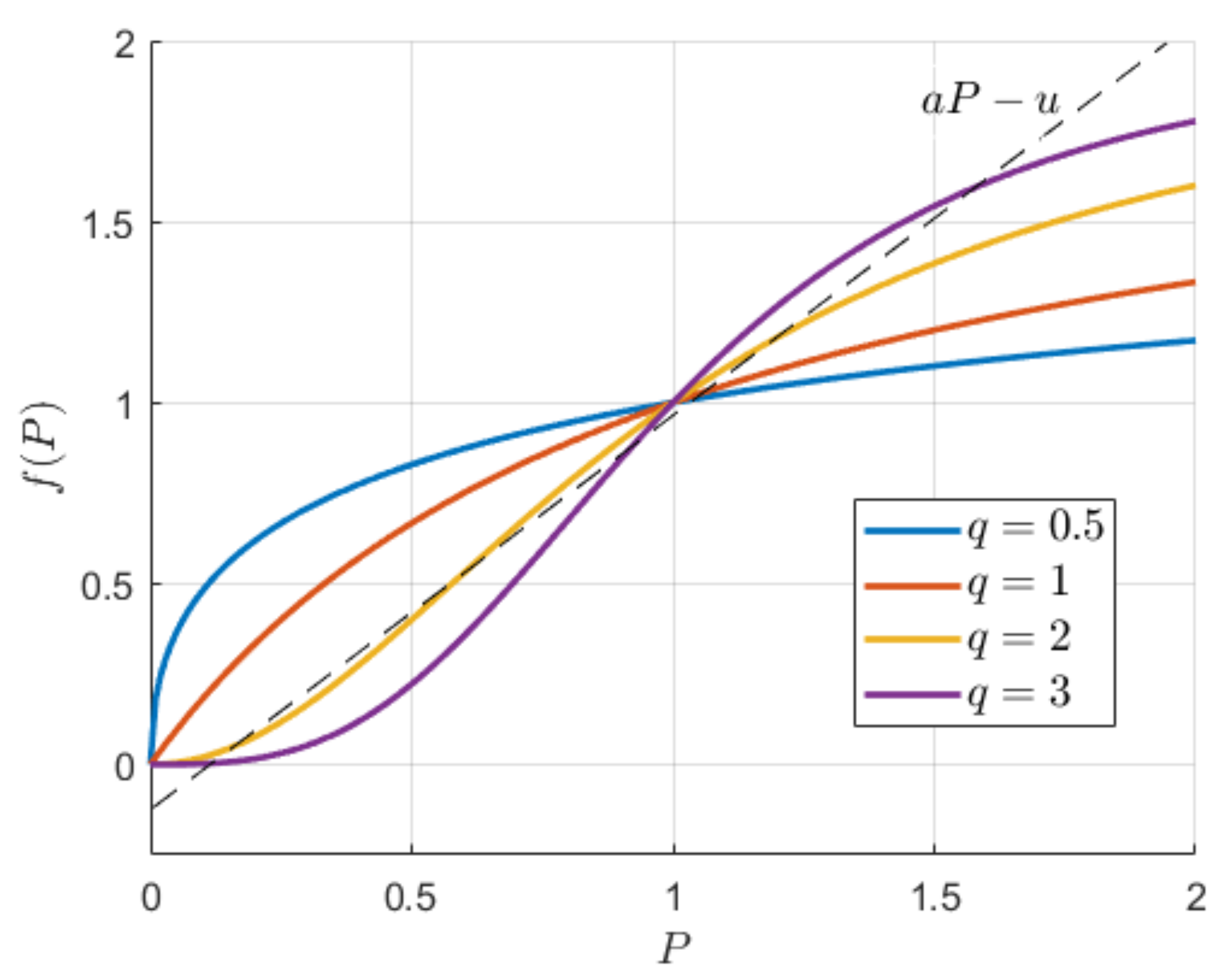
As P grows, $f\left(P\right)$ asymptotically approaches the maximal internal loading rate r. The parameter m determines the level at which the internal loading equals one-half of its maximal value, $r/2$, and q controls the slope of f in a neighbourhood of m (see Figure 1):

$$\frac{\mathrm{d}}{\mathrm{d}P}f\left(P\right)=\frac{qr{m}^q{P}^{q-1}}{{\left(m^q+P^q\right)}^2}\Rightarrow \frac{\mathrm{d}}{\mathrm{d}P}f\left(m\right)=\frac{qr}{4m}.$$

Furthermore, for $q>1$ the function $f\left(P\right)$ is convex-concave, while for $q<1$ this function is strictly concave; its inflection point, at which the function changes its shape from convex to concave, depends on q and asymptotically approaches m as q increases. For $q=2$, the inflection point is located at $x_f=\frac{1}{\sqrt{3}}$. The convex-concave shape of the internal loading function serves as an approximation of the sigmoid relation observed in practice. For $q>1$ and a fixed value of u, the differential Equation (1) has either one or three positive equilibria, while for $q<1$ there is a single positive equilibrium (see Figure 1). For computational reasons, and for analytical tractability, the parameter q is typically assumed to be equal to 2. We will thus use this value if not stated otherwise. Yet, any value of q larger than 2 would not alter the qualitative picture substantially.

By a suitable change of variables—$x=\frac{P}{m}$, $u=\frac{I}{r}$, $a=\frac{(s+h)m}{r}$, and changing the time variable to $t=\frac{r}{m}\tau$—Equation (1) is transformed to the following dimensionless differential equation:

$$\dot{x}\left(t\right)=u\left(t\right)-ax\left(t\right)+\frac{x^2\left(t\right)}{x^2\left(t\right)+1}.$$

(2)

The left diagram of Figure 2 provides a decomposition of the parameter space w.r.t. the number of roots: it shows the regions of the parameter space where the right-hand side of (2) has either one (region I) or three (region II(a,b)) roots. In the latter case, the system (2) has two stable and one unstable equilibria, with the unstable equilibrium being located between the two stable ones, separating the domains of attraction of the stable equilibria. The right diagram shows the emergence and disappearance of steady states for varying values of u for a fixed value of a, here $a=0.51$, viz. it displays a bifurcation diagram for region IIb.

As the parameter u changes, the system (2) undergoes two saddle-node bifurcations, which result in forming what is called a hysteresis loop (see Figure 2, right diagram). This implies that at certain level of the loading rate, the state of the system undergoes an irreversible transition from one stable equilibrium to another one. Suppose that the initial concentration of organic compounds is sufficiently low (the oligotrophic state), that is, the state is located on the lower, blue branch of the curve. As the loading increases, the steady state moves to the right until it arrives at the right tipping point (B). If the loading u grows beyond the critical value, the state jumps to the upper branch of the curve that corresponds to a high concentration of organic compounds (the eutrophic state). Thereafter, a slight decrease in the loading will not suffice for a return to the oligotrophic state. Rather, the lake will stay in the eutrophic state until the loading decreases below the left tipping point (A).

For values of a less than $1/2$, though, the left tipping point moves to the negative half-plane, rendering a return to the initial, oligotrophic state impossible even by stopping the phosphorus inflow completely. Thus, depending on the parameters, we have three types of shallow lake dynamics:

I

reversible;

IIa

irreversible;

IIb

hysteresis.

This model can be extended along several lines. Carpenter [23] distinguished between the concentration of phosphorus in the soil (U), in the lake water (P), and in the bottom sediments (M). Denoting the loading (input) by U, the agricultural and non-agricultural inputs of phosphorus to the watershed by F and W, respectively, and the export of phosphorus from the watershed in farm products by H, the dynamics of the system can be described by three differential equations:

$$\begin{array}{cc}\hfill \dot{U}\left(t\right)& =W+F-H-cU\left(t\right)\hfill \end{array}$$

(3a)

$$\begin{array}{cc}\hfill \dot{P}\left(t\right)& =cU\left(t\right)-(s+h)P\left(t\right)+rM\left(t\right)f\left(P\right(t\left)\right)\hfill \end{array}$$

(3b)

$$\begin{array}{cc}\hfill \dot{M}\left(t\right)& =sP\left(t\right)-bM\left(t\right)-rM\left(t\right)f\left(P\right(t\left)\right),\hfill \end{array}$$

(3c)

where c is the run-off coefficient, b is the burial rate of the sediment, while s and h and $f\left(P\right)$ are the same as in (1a). This model presents an extension of the classical model (1), where the dynamics of the phosphorus in the bottom sediments are explicitly accounted for by the slower changing variable M. If this variable is fixed, (3) reduces to (1).

The equilibrium value of M is given by

$$M^{*}=\frac{sP}{b+rf\left(P^{*}\right)},$$

which is positive for all positive values of $P^{*}$. Furthermore, substitution of $M^{*}$ into the equilibrium equation for P does not change the qualitative structure of the solution. Similarly to (1a), the system (3) can have either one or three equilibria. However, as the number of parameters increases, in comparison to (1a), their qualitative characterization becomes more involved.

2.2. A Stochastic Extension. Indicators of Regime Shifts

Kossioris et al. [24] analysed a stochastic version of (2) in which the recycling rate is randomly perturbed by a linear multiplicative white noise with diffusion strength $\sigma$, yielding the stochastic differential equation

$$\mathrm{d}{x}_t=\left(u_t-b{x}_t+\frac{x_t^2}{x_t^2+1}\right)\mathrm{d}t+\sigma x_t\mathrm{d}{W}_t.$$

(4)

where the term in brackets represents the drift term, and $\mathrm{d}{W}_t$ denotes the increment of a Wiener process (Brownian motion). A particular advantage of this approach is that within the context of dynamic programming, stochastic optimal control problems result in Hamilton–Jacobi–Bellman equations that have the form of a non-linear elliptic PDE for an infinite horizon, resp., a parabolic PDE for a finite horizon. Such PDEs are typically amenable to numerical analysis, see, e.g., Barles and Souganidis [25], Crandall et al. [26].

In contrast to this, Carpenter and Brock [27] considered a stochastic version of (3), where they add to both equations a stochastic term describing the uncertainty related to the transfer of phosphorus from the sediments and soil to the water:

$$\begin{array}{cc}\hfill \mathrm{d}{U}_t& =\left[F_t-cH{U}_t\right]\mathrm{d}t\hfill \end{array}$$

(5a)

$$\begin{array}{cc}\hfill \mathrm{d}{P}_t& =\left[c{U}_t{H}_t-(s+h)P_t+r{M}_{t}f\left(P_t\right)\right]\mathrm{d}t+\sigma M_{t}f\left(P_t\right)\mathrm{d}{W}_t\hfill \end{array}$$

(5b)

$$\begin{array}{cc}\hfill \mathrm{d}{M}_t& =\left[s{P}_t-b{M}_t-r{M}_{t}f\left(P_t\right)\right]\mathrm{d}t-\sigma M_{t}f\left(P_t\right)\mathrm{d}{W}_t.\hfill \end{array}$$

(5c)

That is, P and M follow stochastic processes with drift given by the terms in brackets and with constant volatility $\sigma$. The Wiener process $W_t$ governs both $P_t$ and $M_t$ as the amount of phosphorus that gets recycled from the surface sediment (M) equals the amount of phosphorus taken up by the water (P); and by the same argument, the volatilities of both processes coincide. Here, $H_t$ represents a multiplicative noise related to the transfer of phosphorus from the soil to the lake, governed by the linear stochastic equation $\mathrm{d}{H}_t=\lambda H_t\mathrm{d}{Z}_t$ (driftless geometric Brownian motion), where $\mathrm{d}{Z}_t$ is the increment of a Wiener process, independent of $\mathrm{d}{W}_t$. Solving this stochastic equation for H yields $H_t=H_{0}exp\left(\lambda Z_t-\frac{{\lambda }^2}{2}t\right)$, which then can be substituted into (5b).

Assuming that the true dynamics of the ecosystem are governed by (5a), Carpenter and Brock [27] explored the possibility of predicting a regime shift from the oligotrophic to the eutrophic state by means of the time series data generated by (5a) when one does not know these true dynamics, but (erroneously) assumes a single-equation dynamic linear model. They show that the estimated standard variation of water phosphorus is a leading indicator for a shift from the oligotrophic to eutrophic state, and may thus help reduce phosphorus inputs so as to prevent a significant deteriorations in water quality.

Contamin and Ellison [28] expanded the results obtained by Carpenter and Brock by analysing 6 potential indicators for imminent regime shifts emerging in model (5), and evaluated their importance for the advance warning of regime shifts. The considered indicators are computed on the basis of the observed time-series data and describe the statistical characteristics of the considered process. Specifically, the standard deviations of the phosphorus level $X_t$ computed on the basis of different models are taken as the first three indicators, the fourth indicator is the maximal value in the spectrum of $X_t$, the fifth indicator is a specific parameter of the identified dynamic linear model, and the sixth indicator is the expectation ${\overline{X}}_t$. They showed that the the fourth indicator, i.e., high-frequency variations in the spectral density of the time-series, is the most useful indicator for predicting a possible regime shift. They stressed the importance of estimating the influence of inertia and the inherent volatility of the system on the accuracy of the predictions.

Subsequently, Wang et al. [29] further advanced this topic by developing an approach to detect rising volatility (here for for Erhai Lake, Yunnan, China) before the switching event—to which they refer as flickering—from the sparse data. Flickering refers to a particular pattern of system dynamics characterised by fast jumps between different regions of attraction, cf. Scheffer et al. [30]. Wang et al. argue that flickering can serve as an early warning signal, before the system approaches the border of the safe operating region. For the notion of SOS and its applications in ecology, the reader may consult, for example, [31,32,33].

The concept of safe operating spaces (SOS) has been developed and is frequently used for ecosystems. A SOS is the region of available policies (controls) such that a sustainable steady state can be supported; that is, using the control variable(s) as a bifurcation parameter, the SOS is the domain for which a sustainable steady state exists (possibly bounded by the actual or equilibrium control). This does not necessarily imply, though, that it is optimal to choose a level of the control within the SOS, as it may, for exmaple, be optimal to totally deplete the resource even if a policy exists that supports the sustainable steady state. This is, for example, clearly explained by Carpenter et al. [34].

2.3. Hybrid Model of a Shallow Lake

The internal loading function f, given by (2), can be approximated by a piecewise constant function taking different values for different values of the state variable (see Figure 3). This implies that the shallow lake model can be well approximated by a hybrid model, whose evolution is governed by one of the two linear models corresponding to different levels of phosphorus concentration:

$$\dot{x}\left(t\right)=\left\{\begin{array}{cc}u\left(t\right)+bx\left(x\right)+f_1,\hfill & x<x^{*}\hfill \\ u\left(t\right)+bx\left(x\right)+f_2,\hfill & x>x^{*},\hfill \end{array}\right.$$

(6)

where $f_1$ and $f_2$ are the average values of $f\left(x\right)$ over the intervals of interest. For instance, for $f\left(x\right)=\frac{x^2}{x^2+1}$ and $x\in [0,1]$, we have $f_1={\int }_0^{1}f\left(x\right)dx=1-\frac{\pi }{4}\approx 0.2146$.

Such a formulation allows one to consider the optimal control problem for a shallow lake within the well-developed framework of hybrid systems, as was suggested by Reddy et al. [35] (for further details about hybrid systems see Shaikh and Caines [36], Gromov and Gromova [37] and references therein). The hybrid system framework has the advantage that each single subsystem has linear dynamics and, hence, is easier to analyse. However, the switching condition $x\left(t\right)=x^{*}$ is a state-dependent one, implying that the corresponding hybrid optimal control problem may exhibit jumps in the adjoint variable. This becomes crucial in the case when the number of jumps is infinite.

Reddy et al. [35] analysed the resulting hybrid optimal control and proved that there are only two possible solutions to this problem: the system trajectory converges either to the steady state of the oligotropic subsystem, or to the steady state of a eutrophic subsystem. Which of the two steady states is optimal depends on the system parameters. Also, for a particular initial condition, there appears a Skiba point, which separates the two solutions described above. This result well matches features of the original model, thus confirming the validity of the obtained results. In contrast to the original optimal control problem, which can be analysed only numerically, the solution of the hybrid linear system potentially admits an analytical characterization; specifically, the conditions determining which of the steady states is optimal can be formulated as a set of relatively simple inequalities.

2.4. Discrete-Time Models

The discrete-time version of the shallow lake model was initially introduced by Dechert and Brock [38] in the form

$$x(t+1)=u\left(t\right)+\alpha x\left(t\right)+\frac{x^2\left(t\right)}{1+x{\left(t\right)}^2}.$$

(7)

While the interpretation of these parameters is analogous to their continuous-time counterparts in (2), the specific values for the parameter for the discrete and the continous model generically differ. (Just as the continuous-time interest rate differs from its discrete-time counterpart.) Apart from this, the continuous and the discrete time models exhibit similar behaviour: there can be either one or three steady states, and the optimal solution undergoes a bifurcation as the values of the parameters vary.

Dechert and O’Donnell [39] extended model (7) by considering a multiplicative stochastic disturbance term. Specifically, they assumed that the control input $u\left(t\right)$ is multiplicatively disturbed by $Z(t+1)$, with $Z\left(t\right)\ge 0$ representing i.i.d. random variables with expectation equal to 1. Dechert and O’Donnell studied the influence of the variance of Z on the optimal solution. They showed that while the stochastic disturbance has a positive effect by smoothing the value function, there is a non-zero probability that the system eventually enters the eutrophic region even if the optimal policy corresponding to the oligotrophic state is used.

3. Economic Analysis of the Shallow Lake Model

A shallow lake does not exist on its own and in isolation, but constitutes a part of an ecological-economic system, in which the economic, in particular, agricultural activities of humans, interferes with and may disrupt the ecological functioning of the lake. An important issue is thus to determine the conditions that would allow a balanced and sustainable development of the ecosystem and a quick recovery to such a status once such a balanced status is disturbed (resilience of the ecosystem). To find suitable policies for transition towards a welcome ecological status and for a quick path of recovery, economists typically formulate intertemporal optimization problems, where a decision maker aims at maximizing the net profit (or benefit) consisting of the economic and environmental utility (directly or indirectly) derived from the lake minus the loss due to the decrease in ecological functions of the lake.

Specifically, Mäler et al. [15] considered a discounted infinite horizon optimal control problem with logarithmic utility and quadratic cost function:

$$J\left(u\right)={\int }_0^{\infty }{e}^{-\rho t}\left(lnu\left(t\right)-c{x}^2\left(t\right)\right)\mathrm{d}t.$$

(8)

While the profit function (8) is quite standard in economic analysis, there are complementary approaches aiming at valuing the ecological services of the ecosystem (see, e.g., Barbier [40]).

This model can be easily extended to a dynamic game with n agents or players (e.g., communities, companies, etc.) and strategy variables $u_i$ (for each $i=1,\dots ,n$) contributing to the total loading of the pollutants or nutrients, i.e., $u\left(t\right)={\sum }_{i=1}^n{u}_i\left(t\right)$. In this case, the profit functional (8) is defined separately for each individual agent, $J_i=J\left(u_i\right)$. In such a framework, we may either consider a strategic non-cooperative game where each player chooses the value of its control variable(s), or a cooperative game where players forming coalitions mutually decide on the total utility of or the utility allocation within their coalition. In the first case, the equilibrium concept usually applied is the Nash equilibrium (or some of its later refinements); in the latter case, it is standard to maximize the sum of the utilities of all players within the coalition (provided that utility is transferable).

Mäler et al. [15] introduced an environmental tax $\tau$ imposed on individual phosphorus loadings $u_i$ ($i=1,\dots ,n$) in order to internalize the environmental externalities imposed by each player on the society:

$$J\left(u_i\right)={\int }_0^{\infty }{e}^{-\rho t}\left(ln{u}_i\left(t\right)-\tau \left(t\right)u_i\left(t\right)-c{x}^2\left(t\right)\right)\mathrm{d}t.$$

(9)

The question is then whether it is possible, by a suitable choice of the tax rate, to induce a socially optimal management path. Mäler et al. [15] showed that by an appropriate choice of a time-varying tax $\tau \left(t\right)$, the decision maker can ensure that the Nash equilibrium solution brings about the socially optimal outcome. However, such a scheme requires a continuous adjustment of the tax rate, which is hardly practical and realistic. To overcome this problem, one may impose the optimal steady state tax ${\tau }^{*}$ instead. While this choice guarantees that the Nash equilibrium solution coincides with the socially optimal allocation, the transient time path is generically inefficient – and since this path may take quite a long time, this approach also fails to safeguard efficiency for a considerable period of time.

3.1. Dynamics of Capital Accumulation

The shallow lake model Mäler et al. [15] has been extended in various ways to better describe the economic dynamics governing, or accompanying, the eutrophication of the lake. For example, Heijnen and Wagener [41] extended the model by allowing the removal of phosphorus and distinguishing between production and consumption and thus adding capital as a second state variable, where the inflow of phosphorus is proportional to the installed capital:

$$\dot{k}\left(t\right)=\pi \left(k\left(t\right)\right)-q\left(t\right)-(\delta +\tau p)k\left(t\right),$$

(10)

where k is the per capita capital (which can be normalized in such a way that one unit of capital corresponds to one unit of pollution), $\pi \left(k\right)$ is an increasing and concave production function, q is the consumption, $\delta$ is the capital depreciation rate, p is the cost of trapping a unit of pollution, and $\tau \in [0,1]$ is an adjustable parameter that corresponds to the fraction of collected pollutant. The rate of consumption $q\left(t\right)$ is now considered as a controlled input, while the loading $u\left(t\right)$ is expressed as $u\left(t\right)=(1-\tau )k\left(t\right)$, i.e., (2) turns into

$$\dot{x}\left(t\right)=(1-\tau )k\left(t\right)-bx\left(t\right)+\frac{x^2\left(t\right)}{x^2\left(t\right)+1}.$$

The profit functional then writes as

$$J\left(u\right)={\int }_0^{\infty }{e}^{-\rho t}\left(lnq\left(t\right)-c{x}^2\left(t\right)\right)dt,$$

(11)

i.e., one aims at maximizing the logarithm of consumption while bearing the costs proportional to the square of the pollution stock.

Using this framework, Heijnen and Wagener [41] examined the optimal taxation of emissions of pollutant when the tax revenue is used by the government for the removal of phosphorus. They show that an optimal but time-independent abatement level can avoid catastrophic regime shifts for a competitive economy whenever it is socially optimal to avoid those events.

3.2. A Fishery in a Shallow Lake

In another extension of the shallow lake model, Janmaat [42] considered fishing when this activity impairs the health of the habitat. More specifically, Janmaat considered a fish population which follows logistic growth, while the carrying capacity of the habitat diminishes with growing levels of pollution. The fish stock is subject to harvesting, which leads to an increase in pollution, e.g., through bottom dragging. The resulting model is thus

$$\begin{array}{cc}\hfill \dot{x}\left(t\right)& =mu\left(t\right)-sx\left(t\right)+\frac{x^2\left(t\right)}{1+x^2\left(t\right)}\hfill \end{array}$$

(12a)

$$\begin{array}{cc}\hfill \dot{z}\left(t\right)& =rz\left(t\right)\left(1-\frac{z\left(t\right)}{K-x\left(t\right)}\right)-qu\left(t\right)z\left(t\right),\hfill \end{array}$$

(12b)

where $x\left(t\right)$ is the stock of pollution (phosphorus), $z\left(t\right)$ is the stock of fish, and $u\left(t\right)$ is the harvesting effort, which is assumed to be proportional to the rate of phosphorus inflow from the sediments that results from bottom dragging. Furthermore, K is the normalized environmental carrying capacity, which decreases with an increase in pollution, and $qu\left(t\right)z\left(t\right)$ is the Schaefer stock-dependent effort productivity function, where $q\in (0,1)$ is the proportion of the total fish stock available for harvesting.

The instantaneous profit function is assumed to be the (discounted) difference between the market price of the harvested fish and the cost of harvesting:

$$J\left(u\right)={\int }_0^{\infty }{e}^{-\rho t}\left[p\left(qu\right(t\left)z\right(t\left)\right)qu\left(t\right)z\left(t\right)-c\left(u\right(t\left)\right)\right]dt,$$

(12c)

where $p(·)$ is the price function, which in general may depend on the amount of harvested fish. The problem (12) results in a highly non-linear canonical system that has been only partially studied using numerical methods.

4. Qualitative Analysis of the Optimal Control Problem

The qualitative analysis of the considered optimal control problems is of the utmost importance, as it allows the decision maker to make informed decisions about the choice of the policy-related parameters. A particular challenge results from the fact that small variations in the parameters may yield substantial structural changes, namely qualitative changes in the structure of the steady states. For example, a small change in the growth function, in the discount rate, or the tax rate, may change the number and the stability of the steady states, possibly destabilizing an up to now stable steady state, or vice versa. Bifurcation analysis may help identify the values of the parameters for which such structural changes emerge.

While the formal analysis of the existence of solutions to the optimal control problem (2), (8) has been carried out only recently, in Bartaloni [43], initial qualitative results were presented already in the very first papers devoted to the problem. Specifically, Mäler et al. [15] and Brock and Starrett [14] demonstrated that for a certain range of parameters, the optimal control problem (2), (8) has two distinct open-loop (Nash) equilibrium solutions: one corresponding to the oligotrophic mode and one corresponding to the eutrophic one. Between these two equilibria, there may exist Skiba points, which are characterized by the property that it is equally optimal to move to either equilibrium point from there Skiba [44].

When the control increases, the marginal utility decreases (decreasing marginal utility), while the marginal cost increases. This implies that in the situation when two equilibria coexist, the eutrophic equilibrium yields the lower value of the profit function, see (Wagener [45] Section 3). In a non-cooperative scenario the situation becomes more pronounced with an increased number of players. Brock and de Zeeuw [46] showed that such “bad” Nash equilibria can be beneficial within a repeated game, since this equilibrium may be used as a threat point as part of a trigger strategy. In this case, the “bad” equilibrium may facilitate or even render possible to sustain cooperation, and thus to accomplish a “good status”, even when the future is strongly discounted by the players. Wagener [45] extended this analysis by computing the minimal discount factors for which the “bad” Nash equilibrium acts as a trigger.

The problem of multiple equilibria in the infinite horizon optimal control problem (2), (8) was thoroughly studied by Wagener [47]. He showed that the resulting canonical system has either a single saddle point equilibrium, which corresponds to a unique solution, or two saddle points and a single unstable focus located in between. The transition between one and three equilibria is characterized by a saddle-node bifurcation, which results in a fusion and a subsequent annihilation of one saddle point and the unstable focus.

As for the region with three equilibrium points and the initial stock of pollution located between the saddle point equilibria (i.e., the lake is neither over polluted, nor ideally clean), three situations may occur. The trajectories leaving the unstable focus may coincide with the stable manifold of either one of the saddle points or both. In the first case, the stable manifold, “trapped” by the unstable focus, is not optimal, while the second one corresponds to the optimal solution. Depending on which stable manifold is left “free”, the optimal solution may correspond to either the oligotrophic or the eutrophic mode. In the second case, both stable manifolds are tied to the unstable focus and, hence, which stable manifold is optimal depends on the initial condition. As the payoff function depends continuously on the initial condition, there exists a point such that either stable manifold yields the same value of the payoff function. Such a point is called a Skiba or indifference point. The three subcases—the optimal oligotrophic, the optimal eutrophic, and the mixed one—are separated by the regions of the parameter space where heteroclinic bifurcations occur. There are two such bifurcations, where the heteroclinic connection is directed from the left saddle point to the right one, or the other way around.

The described qualitative picture is generic and will appear, with some modifications, in many similar situations. The obtained results were further refined by Kiseleva and Wagener [48], where the higher-dimensional bifurcations were identified and a sensitivity analysis for the previously obtained regions of the parameter space was carried out.

Grass et al. [49] extended the shallow lake model (3) by including, beyond the accumulation process of phosphorus in the water, the slow accumulation of phosphorus in the surface sediment. The later process determines the dynamics of recycling phosphorus back into the water. In this way, the canonical system for the optimal control problem (3), (8) becomes 4-dimensional, bringing about new phenomena: Grass et al. demonstrated that there appears a new type of Skiba point such that the trajectories that leave these points converge to the same steady state. Furthermore, the manifolds separating different regions of the parameter space become 2-dimensional and their geometry becomes more involved. However, the employed extension does not change the qualitative picture described above: The system may still have either one optimal solution (Nash equilibrium point), or two solutions corresponding to the oligotrophic and eutrophic modes of operation of the lake. In the latter case, one of the solutions dominates, with exception of the Skiba points, which correspond to the equally optimal solutions.

The above problem can be approached in two different ways. Either it can be viewed as an optimal control problem with fast and slow dynamics, and can then be solved by using the timescale separation techniques (see, for example, [50]); or it can be viewed as a general 4-dimensional canonical system, which can be solved by means of the existing results for 4D canonical systems, going back to Dockner [51]. Subsequently, Tahvonen [52], Wirl [53,54] and others built upon [51] and applied the developed methods to problems in resource economics. Notably, Wirl [54] applied the results of Dockner [51] to explore the possibilities of thresholds and cycles in a consumption–production–pollution model.

In contrast to the previously mentioned papers, where the open-loop optimal solutions are obtained using the celebrated Pontryagin maximum principle [55], Kossioris et al. [56] characterized the Nash equilibrium solutions to (2), (8) using Bellman’s dynamic programming [57]. A particular feature of the obtained Hamilton–Jacobi–Bellman (HJB) equation is that there is no terminal condition, which indicates that there may exist multiple solutions. Therefore, one has to single out a specific class of optimal solutions for which the system state converges to an equilibrium. This imposes an additional condition on the problem that renders the problem well-posed and then allows numerical solution. Subsequently, Kossioris et al. [58] extended the model of Kossioris et al. [56]: To determine the optimal state-dependent taxation rate, they thoroughly analysed the associated HJB equation and found that by a proper choice of taxation scheme, the feedback Nash equilibrium can be shifted toward the socially optimum solution. However, within the considered framework, the feedback Nash equilibrium always performed worse than the socially optimal control, which agrees with intuition.

5. Practical Applications

There have been numerous studies aimed at applying various theoretical methods to the analysis of specific ecological systems. Such studies bridge the gap between theory and practice and help to inform the restoration policies being developed for specific ecological systems. Below, we present a brief overview of several research directions. However, we consider only those studies that are based upon the use of mathematical methods; we omit purely empirical studies. For the latter, we refer the interested reader to Søndergaard et al. [59].

5.1. Forecasting Lake Dynamics

Carpenter [23] carried out extensive numerical simulations of the shallow lake model (3) using the values of parameters previously estimated by Bennett et al. [60] for the watershed of Lake Mendota, WI, USA. Carpenter showed that although eutrophication is reversible, this process may require a time that exceeds a human lifetime, unless substantial changes in soil management are made. In view of this, analysis exclusively focusing on steady states arguably ignores the ecologically, economically and politically significant transition periods, with which we will have to cope with for many years, if not decades. In this vein, Carpenter and Lathrop [61], providing an overview of empirical studies of eutrophication, analysed different processes leading to the transition from an oligotrophic to a eutrophic state.

5.2. Estimation of the Thresholds in Lake Dynamics

While shallow lake dynamics offers valuable insights into the nature and characteristic properties of regime shifts in systems with thresholds, the problem of estimating the levels and probabilities of these thresholds is of the utmost importance. There is a wide range of statistical, empirical, and analytical techniques developed for analysing ecological regime shifts, e.g., Andersen et al. [62]. Specifically, Carpenter and Lathrop [61] used the phosphorus dynamics (1) and the observations of the phosphorus budget of Lake Mendota for the last 30 years to estimate the probability distribution of the threshold for eutrophication and formulated suggestions for designing management strategies. Liang et al. [63] specified 4 simple models with time-driven switching to identify the possibility of shifts in the nutrients–phytoplankton relationship in lakes. They identified a change in this relationship and showed that an increase in nutrients did not drive this change, while total phosphorus (TP) plays a more important role than total nitrogen in an increase in Chlorophyll a; and reducing nutrients is a better strategy than ecosystem recovery to effectively reduce the concentration of Chlorophyll a. Likewise, Yao et al. [64] used a multidimensional similarity cloud model to assess the level of eutrophication on the basis of different indicators, including phosphorus concentration and chlorophyll levels. The developed method was used to evaluate the degree of eutrophication of Nansi Lake in Shandong Province, China.

Even though some authors have been able to identify thresholds in the data, this is generally a quite challenging task: Firstly, data and measurement techniques might be insufficient to determine any thresholds. Secondly, since thresholds do not affect the state variables directly, but only the dynamical systems governing their motion, i.e., their time derivatives, the state variables evolve continuously even at thresholds: natura non facit saltus. Thirdly, our notion of a threshold is a modelling device and thus an approximation—hopefully a suitable one—of nature. It thus comes as a little surprise, at least to us, that in a recent meta analysis, Hillebrand et al. [65] hardly found any systematic quantitative evidence for statistically identifiable transgressions of ecological thresholds.

5.3. Economic Analysis

Hein [66] studied the system of the 4 largest lakes in the De Wieden wetland, located in the northeastern part of the Netherlands. The study compared the costs and benefits obtained from the application of different eutrophication control measures. The performed analysis suggested specific measures to reach clear water and evaluated the associated costs. Specifically, it was estimated that the most cost-efficient way to achieve a backward shift to the oligotrophic state would amount to reducing the phosphorus loading by three tons/year and reducing the population of benthovorous fish. The cost of this investment is evaluated to be around 5 mln. euros/year while the benefits of reaching the oligotrophic state are estimated to be at least 0.75 mln. euros/year. Subsequently, Deng et al. [67] presented the results of an economic analysis aiming at balancing economic growth and the reduction of harmful emissions, with an application to the Poyang Lake watershed, China. Using an integrated computable general equilibrium model along with social accounting matrices (see Horridge and Wittwer [68] for details), Deng et al. analysed the effects of different taxation schemes for the control of the lake eutrophication and concluded that it is more efficient to introduce a sufficiently high, 6%, tax on the agricultural sector (which is the main pollutant), rather than imposing lower, 1–2%, taxes on a group of industries that potentially contribute to the pollution (agriculture, mining, livestock etc.).

Jiang et al. [69] presents an example of a cost-efficiency analysis that seeks to find a trade-off between the economic and ecological costs resulting from wastewater treatment and the reduction in ecosystem services. The paper presents the results for the data from Lake Taihu, China. Their results underline the importance of the accurate valuation of ecosystem services, for a low economic valuation—and for this reason an underestimation—may lead to substantial damage to the ecosystem. Furthermore, they stress the significance of the amount of the water in the lake and the need for the control of water consumption: An excessive water consumption leads to an increase in pollutant concentration.

Xu et al. [70] use a vegetation growth model that presents an alternative to the standard shallow lake model (2). This model possesses similar qualitative properties as (2), but is less amenable to analysis due to its highly non-linear structure. Using the data estimated for Lake Baiyangdian from the North China Plain and numerical simulations, they perform a sensitivity analysis of different scenarios of the lake’s evolution. This analysis demonstrated that there is a strong correlation between the concentration of phosphorus and the vegetation coverage, thus confirming the previously obtained results. Moreover, the hydrological connectivity of the lake and the structure of the macrophyte population strongly influence the eutrophication process.

We also mention the paper by Mooij et al. [71] where they present an overview of extremely complex dynamic models aiming at providing a detailed description of the whole ecosystem of a lake in all its complexity. Yet, while such models are supposed to account for all processes that influence the dynamics of a shallow lake and the surrounding ecosystem, they are typically difficult to interpret and are hardly amenable to a qualitative analysis.

6. Discussion

This survey confirms that the qualitative analysis of the dynamics and the management of shallow lake-based ecological systems remains a vibrant research topic, even 20 years after it was initiated. A detailed qualitative analysis of the optimal control problem for a shallow lake has been carried out both for cooperative and non-cooperative scenarios. The shallow lake model has been extended along several directions: Either by extending the shallow lake model itself (by increasing the number of differential equations or by adding stochastic terms), or by augmenting the basic dynamics (2) with equations describing various accompanying processes (fishing, capital accumulation etc.) Many important conclusions have been drawn from the analysis of these models. Specifically, the carried out analyses helped to better understand the role of two equilibria: An oligotrophic and a eutrophic one, and the complex interplay between them, within the context of sustainable development policies.

On the other hand, it is also noticeable that there are several problems that still largely remain unanswered. First, the majority of the qualitative results were obtained for a specific class of optimal control problems with the profit functional in the form of (8) or (9). While this formulation presents a realistic approximation of the net profit, a comparison with other forms of the profit functional is missing. In addition, there is still a gap between the large number of empirical studies and the analysis based upon the use of analytical methods.

References

- Scheffer, M.; Carpenter, S.; Foley, J.A.; Folke, C.; Walker, B. Catastrophic shifts in ecosystems. Nature 2001, 413, 591–596. [Google Scholar] [CrossRef]
- Rocha, J.C.; Peterson, G.; Bodin, Ö.; Levin, S. Cascading regime shifts within and across scales. Science 2018, 362, 1379–1383. [Google Scholar] [CrossRef]
- Cottrell, R.S.; Nash, K.L.; Halpern, B.S.; Remenyi, T.A.; Corney, S.P.; Fleming, A.; Fulton, E.A.; Hornborg, S.; Johne, A.; Watson, R.A.; et al. Food production shocks across land and sea. Nat. Sustain. 2019, 2, 130–137. [Google Scholar] [CrossRef]
- Reyers, B.; Folke, C.; Moore, M.L.; Biggs, R.; Galaz, V. Social-ecological systems insights for navigating the dynamics of the Anthropocene. Annu. Rev. Environ. Resour. 2018, 43, 267–289. [Google Scholar] [CrossRef]
- Elmqvist, T.; Andersson, E.; Frantzeskaki, N.; McPhearson, T.; Olsson, P.; Gaffney, O.; Takeuchi, K.; Folke, C. Sustainability and resilience for transformation in the urban century. Nat. Sustain. 2019, 2, 267–273. [Google Scholar] [CrossRef]
- Walker, B. Resilience: What it is and is not. Ecol. Soc. 2020, 25. [Google Scholar] [CrossRef]
- Le Moal, M.; Gascuel-Odoux, C.; Ménesguen, A.; Souchon, Y.; Étrillard, C.; Levain, A.; Moatar, F.; Pannard, A.; Souchu, P.; Lefebvre, A.; et al. Eutrophication: A new wine in an old bottle? Sci. Total Environ. 2019, 651, 1–11. [Google Scholar] [CrossRef] [Green Version]
- Somlyódy, L.; Van Straten, G. Modeling and Managing Shallow Lake Eutrophication: With Application to Lake Balaton; Springer: Berlin, Germany, 1986. [Google Scholar]
- Carpenter, S.R. (Ed.) Complex Interactions in Lake Communities; Springer: Berlin, Germany, 1988. [Google Scholar] [CrossRef]
- Scheffer, M. Ecology of Shallow Lakes; Population and Community Biology Series; Springer: Berlin, Germany, 2004; Volume 22. [Google Scholar]
- Carpenter, S.R.; Ludwig, D.; Brock, W.A. Management of Eutrophication for Lakes Subject to Potentially Irreversible Change. Ecol. Appl. 1999, 9, 751–771. [Google Scholar] [CrossRef]
- Ludwig, D.; Jones, D.D.; Holling, C.S. Qualitative analysis of insect outbreak systems: The spruce budworm and forest. J. Anim. Ecol. 1978, 47, 315–332. [Google Scholar]
- Ludwig, D.; Walker, B.; Holling, C.S. Sustainability, stability, and resilience. Conserv. Ecol. 1997, 1. [Google Scholar] [CrossRef]
- Brock, W.A.; Starrett, D. Managing systems with non-convex positive feedback. Environ. Resour. Econ. 2003, 26, 575–602. [Google Scholar] [CrossRef]
- Mäler, K.G.; Xepapadeas, A.; De Zeeuw, A. The economics of shallow lakes. Environ. Resour. Econ. 2003, 26, 603–624. [Google Scholar] [CrossRef]
- de Zeeuw, A. Regime shifts in resource management. Annu. Rev. Resour. Econ. 2014, 6, 85–104. [Google Scholar] [CrossRef]
- Scheffer, M.; Carpenter, S.R. Catastrophic regime shifts in ecosystems: Linking theory to observation. Trends Ecol. Evol. 2003, 18, 648–656. [Google Scholar] [CrossRef]
- Biggs, R.; Carpenter, S.R.; Brock, W.A. Turning back from the brink: Detecting an impending regime shift in time to avert it. Proc. Natl. Acad. Sci. USA 2009, 106, 826–831. [Google Scholar] [CrossRef] [Green Version]
- Crépin, A.S.; Biggs, R.; Polasky, S.; Troell, M.; De Zeeuw, A. Regime shifts and management. Ecol. Econ. 2012, 84, 15–22. [Google Scholar] [CrossRef]
- Hastings, A.; Abbott, K.C.; Cuddington, K.; Francis, T.; Gellner, G.; Lai, Y.C.; Morozov, A.; Petrovskii, S.; Scranton, K.; Zeeman, M.L. Transient phenomena in ecology. Science 2018, 361. [Google Scholar] [CrossRef] [Green Version]
- Gesztelyi, R.; Zsuga, J.; Kemeny-Beke, A.; Varga, B.; Juhasz, B.; Tosaki, A. The Hill equation and the origin of quantitative pharmacology. Arch. Hist. Exact Sci. 2012, 66, 427–438. [Google Scholar] [CrossRef]
- Holling, C.S. The functional response of invertebrate predators to prey density. Mem. Entomol. Soc. Can. 1966, 98, 5–86. [Google Scholar] [CrossRef]
- Carpenter, S.R. Eutrophication of aquatic ecosystems: Bistability and soil phosphorus. Proc. Natl. Acad. Sci. USA 2005, 102, 10002–10005. [Google Scholar] [CrossRef] [Green Version]
- Kossioris, G.T.; Loulakis, M.; Souganidis, P.E. The deterministic and stochastic shallow lake problem. In Probability and Analysis in Interacting Physical Systems; Friz, P., König, W., Mukherjee, C., Olla, S., Eds.; Springer: Berlin, Germany, 2019; pp. 49–74. [Google Scholar] [CrossRef] [Green Version]
- Barles, G.; Souganidis, P.E. Convergence of approximation schemes for fully nonlinear second order equations. Asymptot. Anal. 1991, 4, 271–283. [Google Scholar] [CrossRef]
- Crandall, M.G.; Ishii, H.; Lions, P.L. User’s guide to viscosity solutions of second order partial differential equations. Bull. Am. Math. Soc. 1992, 27, 1–67. [Google Scholar] [CrossRef] [Green Version]
- Carpenter, S.R.; Brock, W.A. Rising variance: A leading indicator of ecological transition. Ecol. Lett. 2006, 9, 311–318. [Google Scholar] [CrossRef]
- Contamin, R.; Ellison, A.M. Indicators of regime shifts in ecological systems: What do we need to know and when do we need to know it. Ecol. Appl. 2009, 19, 799–816. [Google Scholar] [CrossRef] [Green Version]
- Wang, R.; Dearing, J.A.; Langdon, P.G.; Zhang, E.; Yang, X.; Dakos, V.; Scheffer, M. Flickering gives early warning signals of a critical transition to a eutrophic lake state. Nature 2012, 492, 419–422. [Google Scholar] [CrossRef] [PubMed]
- Scheffer, M.; Bascompte, J.; Brock, W.A.; Brovkin, V.; Carpenter, S.R.; Dakos, V.; Held, H.; Van Nes, E.H.; Rietkerk, M.; Sugihara, G. Early-warning signals for critical transitions. Nature 2009, 461, 53–59. [Google Scholar] [CrossRef] [PubMed]
- Rockström, J.; Steffen, W.; Noone, K.; Persson, A.; Chapin, F.S., III; Lambin, E.F.; Lenton, T.M.; Scheffer, M.; Folke, C.; Schellnhuber, H.J.; et al. A safe operating space for humanity. Nature 2009, 461, 472–475. [Google Scholar] [CrossRef] [PubMed]
- Rockström, J.; Steffen, W.; Noone, K.; Persson, A.; Chapin, F.S., III; Lambin, E.; Lenton, T.M.; Scheffer, M.; Folke, C.; Schellnhuber, H.J.; et al. Planetary boundaries: Exploring the safe operating space for Humanity. Ecol. Soc. 2009, 14. [Google Scholar] [CrossRef]
- Hughes, T.P.; Carpenter, S.; Rockström, J.; Scheffer, M.; Walker, B. Multiscale regime shifts and planetary boundaries. Trends Ecol. Evol. 2013, 28, 389–395. [Google Scholar] [CrossRef]
- Carpenter, S.R.; Brock, W.A.; Hansen, G.J.A.; Hansen, J.F.; Hennessy, J.M.; Isermann, D.A.; Pedersen, E.J.; Perales, K.M.; Rypel, A.L.; Sass, G.G.; et al. Defining a Safe Operating Space for inland recreational fisheries. Fish Fish. 2017, 18, 1150–1160. [Google Scholar] [CrossRef]
- Reddy, P.; Schumacher, J.; Engwerda, J. Optimal management with hybrid dynamics—The shallow lake problem. In Mathematical Control Theory I; Springer: Berlin, Germany, 2015; pp. 111–136. [Google Scholar] [CrossRef]
- Shaikh, M.S.; Caines, P.E. On the hybrid optimal control problem: Theory and algorithms. IEEE Trans. Autom. Control 2007, 52, 1587–1603. [Google Scholar] [CrossRef]
- Gromov, D.; Gromova, E. On a Class of Hybrid Differential Games. Dyn. Games Appl. 2017, 7, 266–288. [Google Scholar] [CrossRef]
- Dechert, W.D.; Brock, W. The Lake Game; Technical Report 24; Wisconsin Madison-Social Systems: Madison, WI, USA, 2003. [Google Scholar]
- Dechert, W.D.; O’Donnell, S.I. The stochastic lake game: A numerical solution. J. Econ. Dyn. Control 2006, 30, 1569–1587. [Google Scholar] [CrossRef]
- Barbier, E.B. Valuing ecosystem services as productive inputs. Econ. Policy 2007, 22, 178–229. [Google Scholar] [CrossRef]
- Heijnen, P.; Wagener, F.O.O. Avoiding an ecological regime shift is sound economic policy. J. Econ. Dyn. Control 2013, 37, 1322–1341. [Google Scholar] [CrossRef]
- Janmaat, J.A. Fishing in a Shallow Lake: Exploring a Classic Fishery Model in a Habitat with Shallow Lake Dynamics. Environ. Resour. Econ. 2012, 51, 215–239. [Google Scholar] [CrossRef]
- Bartaloni, F. Existence of Solutions to Shallow Lake Type Optimal Control Problems. J. Optim. Theory Appl. 2020, 185, 384–415. [Google Scholar] [CrossRef]
- Skiba, A.K. Optimal growth with a convex-concave production function. Econom. J. Econom. Soc. 1978, 46, 527–539. [Google Scholar] [CrossRef]
- Wagener, F. Shallow lake economics run deep: Nonlinear aspects of an economic-ecological interest conflict. Comput. Manag. Sci. 2013, 10, 423–450. [Google Scholar] [CrossRef] [Green Version]
- Brock, W.A.; de Zeeuw, A. The repeated lake game. Econ. Lett. 2002, 76, 109–114. [Google Scholar] [CrossRef]
- Wagener, F.O.O. Skiba points and heteroclinic bifurcations, with applications to the shallow lake system. J. Econ. Dyn. Control 2003, 27, 1533–1561. [Google Scholar] [CrossRef]
- Kiseleva, T.; Wagener, F.O. Bifurcations of optimal vector fields in the shallow lake model. J. Econ. Dyn. Control 2010, 34, 825–843. [Google Scholar] [CrossRef] [Green Version]
- Grass, D.; Xepapadeas, A.; de Zeeuw, A. Optimal management of ecosystem services with pollution traps: The lake model revisited. J. Assoc. Environ. Resour. Econ. 2017, 4, 1121–1154. [Google Scholar] [CrossRef] [Green Version]
- Crépin, A.S. Using fast and slow processes to manage resources with thresholds. Environ. Resour. Econ. 2007, 36, 191–213. [Google Scholar] [CrossRef]
- Dockner, E. Local stability analysis in optimal control problems with two state variables. In Optimal Control Theory and Economic Analysis; Feichtinger, G., Ed.; North-Holland: Amsterdam, The Netherlands, 1985; Volume 2. [Google Scholar]
- Tahvonen, O. On the dynamics of renewable resource harvesting and pollution control. Environ. Resour. Econ. 1991, 1, 97–117. [Google Scholar]
- Wirl, F. The cyclical exploitation of renewable resource stocks may be optimal. J. Environ. Econ. Manag. 1995, 29, 252–261. [Google Scholar] [CrossRef]
- Wirl, F. Sustainable growth, renewable resources and pollution: Thresholds and cycles. J. Econ. Dyn. Control 2004, 28, 1149–1157. [Google Scholar] [CrossRef]
- Pontryagin, L.S.; Boltyanskii, V.G.; Gamkrelidze, R.V.; Mishchenko, E.F. Mathematical Theory of Optimal Processes; CRC Press: Boca Raton, FL, USA, 1987. [Google Scholar]
- Kossioris, G.; Plexousakis, M.; Xepapadeas, A.; de Zeeuw, A.; Mäler, K.G. Feedback Nash equilibria for non-linear differential games in pollution control. J. Econ. Dyn. Control 2008, 32, 1312–1331. [Google Scholar] [CrossRef] [Green Version]
- Bellman, R.E.; Dreyfus, S.E. Applied Dynamic Programming; Princeton University Press: Princeton, NJ, USA, 2015. [Google Scholar]
- Kossioris, G.; Plexousakis, M.; Xepapadeas, A.; de Zeeuw, A. On the optimal taxation of common-pool resources. J. Econ. Dyn. Control 2011, 35, 1868–1879. [Google Scholar] [CrossRef] [Green Version]
- Søndergaard, M.; Jeppesen, E.; Lauridsen, T.L.; Skov, C.; Van Nes, E.H.; Roijackers, R.; Lammens, E.; Portielje, R. Lake restoration: Successes, failures and long-term effects. J. Appl. Ecol. 2007, 44, 1095–1105. [Google Scholar] [CrossRef]
- Bennett, E.M.; Reed-Andersen, T.; Houser, J.N.; Gabriel, J.R.; Carpenter, S.R. A phosphorus budget for the Lake Mendota watershed. Ecosystems 1999, 2, 69–75. [Google Scholar] [CrossRef] [Green Version]
- Carpenter, S.R.; Lathrop, R.C. Probabilistic estimate of a threshold for eutrophication. Ecosystems 2008, 11, 601–613. [Google Scholar] [CrossRef]
- Andersen, T.; Carstensen, J.; Hernandez-Garcia, E.; Duarte, C.M. Ecological thresholds and regime shifts: Approaches to identification. Trends Ecol. Evol. 2009, 24, 49–57. [Google Scholar] [CrossRef] [Green Version]
- Liang, Z.; Qian, S.S.; Wu, S.; Chen, H.; Liu, Y.; Yu, Y.; Yi, X. Using Bayesian change point model to enhance understanding of the shifting nutrients–phytoplankton relationship. Ecol. Model. 2019, 393, 120–126. [Google Scholar] [CrossRef]
- Yao, J.; Wang, G.; Xue, B.; Wang, P.; Hao, F.; Xie, G.; Peng, Y. Assessment of lake eutrophication using a novel multidimensional similarity cloud model. J. Environ. Manag. 2019, 248, 109259. [Google Scholar] [CrossRef]
- Hillebrand, H.; Donohue, I.; Harpole, W.S.; Hodapp, D.; Kucera, M.; Lewandowska, A.M.; Merder, J.; Montoya, J.M.; Freund, J.A. Thresholds for ecological responses to global change do not emerge from empirical data. Nat. Ecol. Evol. 2020, 4, 1502–1509. [Google Scholar] [CrossRef]
- Hein, L. Cost-efficient eutrophication control in a shallow lake ecosystem subject to two steady states. Ecol. Econ. 2006, 59, 429–439. [Google Scholar] [CrossRef]
- Deng, X.; Zhao, Y.; Wu, F.; Lin, Y.; Lu, Q.; Dai, J. Analysis of the trade-off between economic growth and the reduction of nitrogen and phosphorus emissions in the Poyang Lake Watershed, China. Ecol. Model. 2011, 222, 330–336. [Google Scholar] [CrossRef]
- Horridge, M.; Wittwer, G. SinoTERM, a multi-regional CGE model of China. China Econ. Rev. 2008, 19, 628–634. [Google Scholar] [CrossRef]
- Jiang, Y.; Dinar, A.; Hellegers, P. Economics of social trade-off: Balancing wastewater treatment cost and ecosystem damage. J. Environ. Manag. 2018, 211, 42–52. [Google Scholar] [CrossRef]
- Xu, C.; Xu, Z.; Liu, H.; Yang, Y.; Yang, Z. Simulating the effects of regulation measures on ecosystem state changes in a shallow lake. Ecol. Indic. 2018, 92, 72–81. [Google Scholar] [CrossRef]
- Mooij, W.M.; Trolle, D.; Jeppesen, E.; Arhonditsis, G.; Belolipetsky, P.V.; Chitamwebwa, D.B.; Degermendzhy, A.G.; DeAngelis, D.L.; Domis, L.N.D.S.; Downing, A.S.; et al. Challenges and opportunities for integrating lake ecosystem modelling approaches. Aquat. Ecol. 2010, 44, 633–667. [Google Scholar] [CrossRef] [Green Version]
Figure 1.
Plot of the function for , , and different values of q. The intersections of the dashed line with the plot of correspond to the equilibria.
Figure 2.
Decomposition of the parameter space w.r.t. the number of roots (left), and the illustration of two saddle-node bifurcations forming a hysteresis loop for (right). In the right panel, blue lines correspond to the stable equilibria of (2), while the red line is formed by unstable ones. The arrows indicate the direction in which the system traverses the equilibrium points as the parameter u changes.
Figure 3.
Piece-wise approximation (blue) of the function (red) over the interval . The values of are and . The switching occurs at , where the approximating function is discontinuous (dashed line).
Publisher’s Note: MDPI stays neutral with regard to jurisdictional claims in published maps and institutional affiliations. |
© 2021 by the authors. Licensee MDPI, Basel, Switzerland. This article is an open access article distributed under the terms and conditions of the Creative Commons Attribution (CC BY) license (https://creativecommons.org/licenses/by/4.0/).
Share and Cite
MDPI and ACS Style
Gromov, D.; Upmann, T. Dynamics and Economics of Shallow Lakes: A Survey. Sustainability 2021, 13, 13763. https://doi.org/10.3390/su132413763
AMA Style
Gromov D, Upmann T. Dynamics and Economics of Shallow Lakes: A Survey. Sustainability. 2021; 13(24):13763. https://doi.org/10.3390/su132413763
Chicago/Turabian StyleGromov, Dmitry, and Thorsten Upmann. 2021. "Dynamics and Economics of Shallow Lakes: A Survey" Sustainability 13, no. 24: 13763. https://doi.org/10.3390/su132413763
Note that from the first issue of 2016, this journal uses article numbers instead of page numbers. See further details here.