Article

Investigating High-Resolution Spatial Wave Patterns on the Canadian Beaufort Shelf Using Synthetic Aperture Radar Imagery at Herschel Island, Qikiqtaruk, Yukon, Canada

by
Kerstin Brembach
1,2,*,
Andrey Pleskachevsky
3 and
Hugues Lantuit
1,4
1
Department of Permafrost Research, Alfred Wegener Institute Helmholtz Center for Polar and Marine Research, 14473 Potsdam, Germany
2
Institute of Geography, University of Kiel, 24118 Kiel, Germany
3
German Aerospace Center (DLR), Maritime Safety and Security Lab Bremen, Am Fallturm 9, 28359 Bremen, Germany
4
Institute of Geosciences, University of Potsdam, 14476 Potsdam, Germany
*
Author to whom correspondence should be addressed.
Remote Sens. 2023, 15(19), 4753; https://doi.org/10.3390/rs15194753
Submission received: 7 August 2023 / Revised: 11 September 2023 / Accepted: 21 September 2023 / Published: 28 September 2023
(This article belongs to the Section Ocean Remote Sensing)

Abstract

:
The Arctic is experiencing the greatest increase in air temperature on Earth. This significant climatic change is leading to a significant positive trend of increasing wave heights and greater coastal erosion. This in turn effects local economies and ecosystems. Increasing wave energy is one of the main drivers of this alarming trend. However, the data on spatial and temporal patterns of wave heights in the Arctic are either coarse, interpolated or limited to point measurements. The aim of this study is to overcome this shortcoming by using remote sensing data. In this study, the Synthetic Aperture Radar (SAR) satellite TerraSAR-X (TS-X) and TanDEM-X (TD-X) imagery are used to obtain sea state information with a high spatial resolution in Arctic nearshore waters in the Canadian Beaufort Sea. From the entire archive of the TS-X/TD-X StripMap mode with coverage around 30 km × 50 km acquired between 2009 and 2020 around Herschel Island, Qikiqtaruk (HIQ), all the ice-free scenes were processed. The resulting dataset of 175 collocated scenes was used to map the significant wave height ( H s ) and to link spatial and temporal patterns to local coastal processes. Sea state parameters are estimated in raster format with a 600 m step using the empirical algorithm CWAVE_EX. The statistics of the H s were aggregated according to spatial variability, seasonality and wind conditions. The results show that the spatial wave climate is clearly related to the dominant wind regime and seasonality. For instance, the aggregation of all the scenes recorded in July between 2009 and 2020 results in an average of 0.82 m H s , while in October the average H s is almost 0.40 m higher. The analysis by wind direction shows that fetch length and wind speed are likely the most important variables influencing the spatial variability. A larger fetch under NW conditions results in a mean wave height of 0.92 m, while waves generated under ESE conditions are lower at 0.81 m on average.

Graphical Abstract

1. Introduction

The Arctic is one of the most impacted regions in the world in terms of climate change. Global warming trends are amplified in the Arctic and the summer sea ice extent is decreasing at an alarming pace [1,2,3,4,5]. The 21st-century projections even suggest a completely sea ice-free Arctic summer before 2050 [6]. A decreasing sea ice extent is associated with a longer open-water season and larger open-water areas [7,8,9], which, in turn, leads to a greater impact by coastal waves [10,11,12,13]. Many authors have reported a significant positive trend in ocean surface wave heights over the last decades [14,15,16,17,18,19].
An increase in wave height poses a serious threat to local communities and has the potential to alter the coastal ecosystem. Arctic coasts are largely made of permafrost. During the open-water season, which typically lasts three to four months, these coasts are vulnerable to erosion [13,20,21,22] at rates of 1 to 5 m a 1 [23]. Larger waves occurring over longer open-water seasons could dramatically enhance the pace of erosion, as has already been observed along the Arctic rim [11,24,25]. The material mobilised by erosion affects marine ecosystems [26] and alters sediment dynamics [27]. Erosion also threatens local settlements and terrestrial infrastructure, and it amplifies the vulnerability of indigenous coastal communities [28]. Increased wave heights can also pose a threat to navigation in coastal waters [29] and endanger traditional travel routes and fishing activities.
To properly assess the impacts of changing wave dynamics in the Arctic coastal zone, it is necessary to understand the drivers and spatial patterns of wave fields. However, spatial wave patterns in the Arctic have rarely been studied at the local scale due to a lack of in situ data. Therefore, wave patterns have mainly been investigated by using wave hindcasts and re-analyses with a resolution cell size of several kilometres [14,15,18,19] or by using isolated point measurements [30].
In recent years, the ongoing development of spaceborne Synthetic Aperture Radar (SAR) technologies, together with the associated data transfer and data processing infrastructures, has enabled a range of possible oceanographic applications using a variety of developed algorithms. Compared to altimetry, SAR scenes have a much larger footprint and allow the estimation of spatial information with pixel spacings down to 1 m (e.g., the TerraSAR-X High-Resolution Spotlight mode [31]). In addition, SAR instruments can observe the Earth’s day and night in most weather conditions, which is a major advantage over optical remote sensing platforms.
Ref. [32] used an empirical approach to develop the CWAVE_ERS algorithm for retrieving sea state parameters from ERS C-Band imagery. Similar algorithms have been developed in the following years, such as CWAVE_S1 [33] and CWAVE_S1_IW [34] for Sentinel-1 C-Band imagery and XWAVE for TS-X/TD-X X-Band imagery [35]. Other approaches are based on machine learning methods, such as support vector machine [36], extreme learning machine [37], decision tree and the random forest algorithms [38], the backpropagation neural network [39], deep residual convolutional neural network [40] and deep learning with artificial neural networks [41]. Using the latest algorithms, a range of integrated sea state parameters can be estimated from SAR imagery with an accuracy comparable to the uncertainty of ground-truth data [42].
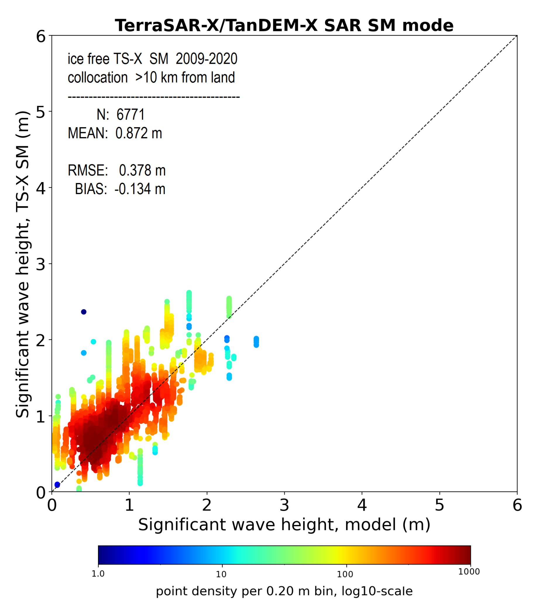
This paper aims to use SAR imagery in the Arctic nearshore zone to provide high-resolution mapping of wave height patterns and to link them to environmental variables, such as wind forcing. In this study, the empirical algorithm CWAVE_EX is used for H s estimation. The algorithm was tuned and validated using wave model hindcasts, WaveWatch-3 and MFWAM, as well as in situ measurements from the National Data Buoy Center (NDBC) by [42]. CWAVE_EX is applied in the Arctic to produce a novel high-resolution dataset of wave heights. The algorithm is able to resolve wave heights on a spatial scale of 600 m in the nearshore zone. The complete processing chain includes a number of steps to achieve high accuracy: denoising, filtering of image artefacts, SAR features estimation and examination, model functions and control of results [42]. CWAVE_EX is applied to the complete ice-free archive of the TerraSAR-X (TS-X) and TanDEM-X (TD-X) scenes over Herschel Island, Qikiqtaruk (HIQ), acquired between 2009 and 2020. Maps of significant wave heights are produced, and H s is analysed for spatial variability, seasonality and wind direction.

2. Materials and Methods

2.1. Study Area

The focus of this study is the Arctic nearshore waters around HIQ at 69.59°N, 139.09°W. HIQ was chosen because of the wealth of ancillary data available to link wave mapping to environmental variables. Previous studies have already linked the highly eroding coast to changes in storm patterns, sea ice coverage and nearshore sediment pathways (e.g., [22,23,43,44,45,46,47]). However, knowledge of the spatial wave climate is crucial to explain the observed erosion rates. Furthermore, HIQ is of high cultural value to the Inuvialuit and is on the tentative list of UNESCO World Heritage Sites submitted by Canada [48]. Coastal erosion poses a threat to this heritage, and one archaeological site has already been lost while other seasonally used buildings needed to be relocated [49]. Knowledge of changing wave patterns and their implications is therefore of great interest to HIQ.
The study area is located in the southern Beaufort Sea and is part of the Yukon–Alaska Beaufort shelf. It is bounded to the east by the Mackenzie Trough, a more than 300 m deep submarine valley approximately 15 km off the coast of HIQ (Figure 1). On the shelf, water depths reach 80 m with a generally gentle seabed. However, close to the northeast coast of HIQ the seabed is much steeper [44]. The island was formed by an ice-push event during the Wisconsin Glaciation. The westward advance of the Laurentide Ice Sheet uplifted material from Herschel Basin to form HIQ [50]. Herschel Basin, located to the southeast of the island, is characterised by water depths of up to 73 m. HIQ is separated from the mainland by Workboat Passage, a shallow water channel about 3 m deep (Figure 1) [51] (p. 188). Workboat Passage is enclosed by the gravel spits Avadlek Spit, Osborn Point and Catton (also called Calton) Point Spit [52].
The Mackenzie Delta 120 km east of HIQ, is the major source of freshwater and sediment in the study area. During the spring and summer, the river discharge results in a thick brackish plume at the ocean surface, some of which is transported westwards towards the island [44,53].
The western and northeastern coastline of HIQ is characterised by steep cliffs of up to 60 m around Collinson Head and Bell Bluff, while the coastal landscape becomes more gentle towards the southeast [54]. HIQ is almost entirely underlain by permafrost. At the coast, this leads to spectacular erosion processes, reflected in the formation of retrogressive thaw slumps and active-layer detachment slides [46,47,48]. Ref. [47] observed an increase in the erosion rates of about 50% between the periods 1970–2000 and 2000–2011. Between 2000 and 2011, the coastal retreat was measured to be 0.68 m/a. The large erosion rates result in an estimated sediment release of about 28.20 m 3 /m [47].
The Arctic is generally micro-tidal, with tides of 10 to 13 cm on the Yukon coast. In comparison, storm surges can exceed this range by up to 3 m and thus have a greater impact on coastal morphology [51] (p. 169).
The climate in the study area is dominated by long, cold winters and short summers. Average monthly temperatures can vary between −25 °C in the coldest months of December to February and 10 °C in the summer months of July and August. Overall, the annual mean temperature is −9.40 °C (1995–2007), with an increase of about 2.50 °C over the last 100 years [43]. The Beaufort Sea is dominated by NW and E winds [44], which are also observed at HIQ. Due to its exposed location, windy conditions exist throughout the year [55].
Significant wave heights in the Beaufort Sea are limited by wind speed and fetch length [17,18]. Therefore, the highest waves occur during the open-water season. This usually starts at the end of June and ends in October, when the fetch can be longer than 1000 km [23]. In general, extreme wave heights in the Beaufort Sea can reach 4 m during storm events [17,56,57]. However, the average wave height is less than 0.8 m high and rarely exceeds 1.20 m [58].
Figure 1. Map of study area. Upper right: Location of the study area near the northernmost border of the United States and Canada. Main map: Location of the study area in the Canadian Beaufort Sea around HIQ in close proximity to the Mackenzie Delta. The bathymetry with Herschel Basin and the Mackenzie Trough is shown in metre depths (Federal Publications, Inc.: Nautical charts of the Beaufort Sea, 1998–2016). Lower left: Study area with geographical names of landscape features. Blue letters indicate maritime and black indicate terrestrial features. The underlain satellite image is a true-colour Sentinel-2 composite acquired 4 August 2021 [59] combined with a hill-shaded 2 m digital surface model.
Remotesensing 15 04753 g001

2.2. Methods

Figure 2 shows an overview of the method flow used in this work and described in the following sections.

2.2.1. SAR

SAR images acquired by the twin satellites TS-X and TD-X were used to map significant wave heights around HIQ. The images were provided by the German Aerospace Centre (DLR). There is no general acquisition schedule for TS-X/TD-X, and each acquisition must be ordered by a user. However, unlike larger open archives, e.g., Sentinel-1, the TS-X/TD-X achieves a higher spatial resolution and allows the study of nearshore areas. TS-X was launched in 2007 and TD-X followed two years later in 2009. Both operate at an altitude of 514 km height in a sun-synchronous orbit with a wavelength of 3.1 cm and a frequency of 9.6 GHz, i.e., X-Band. The satellites have an 11-day repeat cycle. However, the same area can be imaged with different incidence angles on different orbits for up to three days (Table A2). In general, the incidence angles range between 20° and 55° [31]. The satellites observe the Earth in three different main modes: ScanSAR, Strip-Map and SpotLight. This paper focuses exclusively on Strip-Map (SM) data. In contrast to SpotLight images, SM scenes cover the entire nearshore zone around HIQ with a higher spatial resolution than ScanSAR. Operating in the SM mode, the satellite has a fixed antenna beam that illuminates the ground with a continuous sequence of pulses. One scene can have a length of more than 1000 km which is divided into images of variable length. The resulting individual images cover 30 km in the range direction and ca. 50 km in the azimuth direction [60].
In this work, the multi-look ground range-detected (MGD), radiometrically enhanced (RE) SM Level 1 products were used. The scenes have a pixel spacing of approximately 3.30 m in the azimuth direction (flight direction). In contrast to spatially enhanced (SE) products, the RE products are characterised by a higher radiometric accuracy [31]. All ice-free scenes covering the study area between 2009 and 2020 were processed. Specific polarisations were not required, so HH (horizontal transmit–horizontal receive) and VV (vertical transmit–vertical receive) are found in the dataset. Seven different scene footprints with different acquisition frequencies occur within the dataset as a result of ascending and descending satellite paths (Figure 3).

2.2.2. Significant Wave Height Retrieval

Due to its independence from sunlight and cloud coverage, remote sensing SAR data are an indispensable source of 2D ocean surface information for open sea and coastal applications (e.g., [38,61,62,63]). As an active sensor, SAR images the surface roughness while the radar signal returns from the illuminated objects. However, the extraction of the objects from raw SAR data is developed for static targets, while the imaging of non-static targets is associated with the defocusing, smoothing and replacing of the moving objects in the azimuth direction in the resulting SAR image. As a result, SAR imaging of moving waves is associated with several challenges. For instance, in the case of sea states with wavelengths shorter than approximately 80–100 m for TS-X/TD-X SM (depending on the incidence angle and wave amplitude), the azimuth components of individual waves cannot be mapped in a SAR image. This effect is known as the cutoff effect and has been explained by the so-called velocity bunching mechanism [64]. In the TS-X/TD-X images acquired in coastal areas, the sea state falls mainly under the cutoff. Therefore, the waves are mostly too short to be imaged in the resulting SAR scene. However, the information from these short waves is not lost during processing and enters the SAR image in the form of image noise of different characters. A series of SAR image features, e.g., GLCM (Grey-Level Co-occurrence Matrix) parameters such as homogeneity, contrast and spectral-integrated energy for different spectral bands, contain information about these waves and can be returned. The advantage of empirical methods is the possibility of a direct estimation of integrated sea state parameters from SAR features without transforming the image spectrum into a wave spectrum with subsequent integration [42].
In this study, the significant wave height was processed using the empirical algorithm CWAVE_EX developed for the estimation of integrated sea state parameters especially under difficult acquisition conditions (coastal areas, harbours and offshore construction) [34,65,66]. The algorithm is implemented in the Sea State Processor (SSP), which is designed to process SAR data from different satellites and modes in near real time [67]. The full list of TS-X/TD-X scenes used in this study can be found in Appendix A (Table A1) and the generated sea state scenes are available as text files on the ZENODO platform. For more information see Data Availability Statement and Supplementary Materials.
For TS-X/TD-X SM, the CWAVE_EX model functions were developed independently for the HH and VV polarisations. Furthermore, the algorithm was tuned and validated for a total of five satellite modes of the Sentinel-1 C-Band and TS-X X-Band using a set of over 130 SAR features [42]. The estimation of sea state parameters is based on a Normalised Radar Cross-Section (NRCS) analysis of subscenes. One of the basic variables is the SAR image spectrum obtained by Fast Fourier Transformation (FFT) applied to the ground range-detected (GRD), radiometrically calibrated, filtered, denoised, land-masked and normalised subscenes with a size of 1024 × 1024 pixels in the wave-number domain as introduced in [42]. A number of additional SAR features are used to overcome the limitations of non-linear SAR imaging, e.g., the cutoff effect, and to filter spectral signals from objects unrelated to the sea state, such as ships and wakes. All the SAR features estimated from a subscene and used in the model function are of five types:
  • NRCS and NRCS statistics (variance, skewness, kurtosis, etc.).
  • Geophysical parameters (wind speed using the XMOD-2 algorithm for X-Band [68]).
  • GLCM parameters (entropy, correlation, homogeneity, contrast, dissimilarity, energy, etc.).
  • Spectral parameters based on the image spectrum integration of different wavelength domains (0–30 m, 30–100 m, 100–400 m, etc.) and spectral width parameters (Longuet-Higgins spectral width parameter and Goda peakedness parameter).
  • Spectral parameters using products of the normalised image spectrum with an orthonormal functions (CWAVE approach [32]) and the cutoff wavelength estimated using the autocorrelation function (ACF).
When some scenes containing ice (despite visual filtering) enter the processing, the pre-filtering originally designed to remove ship artefacts becomes particularly important. This operation is based on local NRCS statistics and uses a sliding window (sub-subscenes of 150 m × 150 m correspond to average ship sizes). The pixels in the SAR sub-subscene detected as outliers (higher NRCS for ships and lower NRCS for oil or a ship’s wake) are replaced by mean values of the whole subscene. For more details, see [42].
Once the H s has been estimated using the model function, checking the results is again particularly important for regions with the possibility of floating ice. This operation consists of two-step stages based on physical and statistical analysis: the estimated wave height components (dominant swell, secondary swell and windsea) and the local wind speed are checked for agreement. Next, a number of selected SAR features are checked for tolerances. For example, the so-called Rosenthal parameter [42] amplifies the longer wavelength signals by a 1 / k -weighting, where k corresponds to the wavenumber. This means that objects such as ships or ship wakes and ice floes in a subscene significantly increase the value of this parameter and can therefore be filtered out. The estimated H s for the subscene is given the key “bad data” and is not used for further analyses.
As detailed in [42], the processing chain for the calculation of the H s consists of the following steps in the order of their implementation:
  • Radiometric calibration.
  • Scene selection, pre-filtering (ships, ice, oil and wind shadowing artefacts), denoising and normalization.
  • SAR features estimation, control and normalization.
  • The empirical model function to estimate the integrated sea state parameters.
  • Results control (filtering based on physics and statistics, and flagging).
The outputs are generated on a consistent grid with a cell size of 600 m × 600 m. More details on pre-filtering, model functions and control of the results can be found in [42]. Figure 4 shows two processed TS-X scenes under different wind conditions resulting in a moderate (Figure 4a) and relatively smooth (Figure 4b) sea state.
The processed TS-X/TD-X scenes were compared with the results of the spectral wave model hindcast from the global reanalysis WAVERYS (CMEMS) [69,70]. The model results provided with a spatial resolution of 0.2 degrees and 3-hourly steps were spatially and temporally interpolated. The following model data filtering was applied:
  • Land filtering: only data where at least one model grid point (ca. 15 km) separates a SAR subscene from the models land mask were used.
  • Ice filtering: only model data with SWH > 0.01 m were used (ice coverage is indicated by SWH = 0 in the model results).
The comparisons are shown in the scatter plot in Figure 5. As the TS-X/TD-X scenes were processed with a grid step of 600 m, a set of TS-X/TD-X values corresponds to a value of the coarse model. Therefore, the vertical distribution of the wave heights represents the local variability in the sea state.
In total, about 7000 validation samples N were used. The resulting RMSE is 0.37 m (Table 1) and corresponds to the RMSE estimated by validating the SAR sea state algorithm with global data. However, the BIAS associated with the validation of the algorithm is close to zero [42], while this model comparison resulted in an overall BIAS of 0.13 m. This shows an underestimation of the model, especially for sea states below 1 m (Table 1).

2.2.3. Weather Data

Wind data from the weather station on HIQ located at Simpson Point were collected from the climate archive of Environment and Climate Change Canada [71]. The wind speed and wind direction are recorded hourly. The station was installed in 1994 [43], but there have been a few occasions when the station has failed due to weather or wildlife interference. The wind rose in Figure 6 shows the two dominant wind regimes, i.e., NW and ESE, as recorded in the literature [43,44,45]. The wind data were used to aggregate the H s -scenes according to the dominant wind regime.

2.2.4. Statistical Analysis

The H s -dataset retrieved from the SAR imagery was analysed for the entire study area and in Regions of Interest (ROI) according to the wind regime and month (Figure 2). All the H s -scenes were linearly interpolated to a common grid. Hereby, the cell size was increased to 300 × 300 m pixel spacing. False pixel values can occur due to the influence of land on the image spectrum and SAR imaging effects in the shoaling zone [67]. Therefore, a 600 m buffer zone was implemented at the coastline and all the cell values were removed from the analysis. In addition, all the cells that were flagged as false were removed. After filtering, 175 H s -scenes remained, suitable for further analysis.
The entire dataset was analysed according to two changing variables: (1) months and (2) wind regimes. The variable “months” was divided into the classes July, August, September and October, i.e., the open-water season. July contained most of the scenes, while in October only a few scenes were available. This is due to the fact that in October the freeze-up begins [72] and several scenes had to be filtered out.
The variable “wind regime” was divided into the dominant classes E,ESE,SE (abbr. ESE) and NW,NNW,N (abbr. NW), as well as three minor wind regimes WSW,W,WNW (abbr. W), NNE,NE,ENE (abbr. NE) and SSE,S,SSW (abbr. S). The regimes were identified following an analysis of the weather data from Simpson Point, grouping the wind patterns into sectors (Table 2). The occurrence of ocean surface waves depends, among other factors, on the duration of the wind. Therefore, to obtain wave patterns representing the wind direction, stable wind regimes were fixed for each H s -scene. Stable conditions were defined as wind regimes that remained unchanged for at least six hours prior to scene acquisition. The six hours were chosen according to the storm definition used by [10]. As the minor wind regimes (i.e., W, NE and S) were underrepresented in the scene coverage, only the dominant regimes were used for further analysis.
The statistical analysis included basic statistics, such as the mean and standard deviation extraction of stacked H s -scenes. The stacks contained either all the images of the whole dataset or classes according to the variables, i.e., months and wind regimes.
The classes of each variable were tested for significant differences using the Kruskal–Wallis and Dunn’s tests from Scipy: https://scipy.org/ (accessed on 27 September 2023) package version 1.9.1. The mean H s values over each subclass per grid cell were treated as independent data groups. If the alternative hypothesis of the Kruskal–Wallis test was true (significance level α of 0.05), i.e., at least one group differed significantly from another, the Dunn’s test was used. This test determines which groups differ from each other by calculating the z-statistic for each pair. The Bonferroni adjustment was also used to control for the family-wise error rate that can occur when performing multiple comparisons [73].
Seven ROIs were selected to investigate the spatial variability within the entire H s -dataset as well as according to the variables months and wind regime. Each ROI is 5 × 5 pixels in size, covering an area of 1.5 × 1.5 km. Six ROIs (1–5, 7) are located in the nearshore waters around HIQ and Catton Point, while one ROI (6) is located offshore north of the island (Figure 7).
Throughout the data stack, the H s values within each ROI were averaged per scene. In the next step, the averaged H s values were summed up and divided by the total number of scenes. The resulting mean significant wave heights per ROI were compared using the Kruskal–Wallis and Dunn’s tests. Each ROI was treated as one group resulting in 7 groups of 175 measurements (total number of scenes). A similar procedure was used for the variable analysis. In this case, the Kruskal–Wallis and Dunn’s tests were applied to the ROIs within each class rather than between the variables.

3. Results

3.1. Significant Wave Height

Across the study area, the mean H s for the entire H s -dataset is 0.90 m and the averaged standard deviation, i.e., the standard error, is 0.38 m. The relatively high standard error within Workboat Passage is most likely due to the shallow water depth (<3 m), which can lead to a misinterpretation of the wave heights in the SAR scene [67]. The mean H s (Figure 8a) shows the spatial differences around HIQ. The enclosed areas of Workboat Passage and Thetis Bay experience a lower H s in contrast to the areas facing open water. Figure 8b shows that the standard deviation is relatively uniform in the vicinity of HIQ. However, to the northwest, the standard deviation values are slightly higher and this pattern is also visible in the offshore water.
These results are reflected in the ROI statistics. Table 3 shows the mean and standard deviation for each ROI. ROI 5 located in Thetis Bay records the lowest H s value of 0.77 m. The ROIs with the highest mean H s of over 1 m are located in the north of the island with ROI 2, ROI 3 and ROI 6. On the west side of HIQ, ROI 1 has the second lowest H s value with 0.93 m compared to the northeast/east around Bell Bluff and Collinson Head. Here, H s ranges between 0.98 and 0.99 m. Towards the mainland, ROI 7 shows high H s values with 1.03 m, especially compared to Thetis Bay a few kilometres to the north. The standard deviation in Table 3 is lowest southeast of HIQ in ROI 7 with 0.27 m. In contrast, the standard deviation northwest/north of the island ranges between 0.38 and 0.44 m with increasing values towards the offshore waters from ROI 1 and 2 to ROI 6.
Across the dataset, the Dunn’s test shows no significant difference between most ROIs. However, the test shows that the significant wave heights in Thetis Bay are significantly different from all the other ROI wave heights.

3.2. Significant Wave Height according to Wind Regimes

Figure 9 shows the spatial distribution of the mean H s by the wind regime. The most frequent wind regimes ESE and NW show opposite wave patterns. During easterly winds, H s is higher on the east side and lower on the west side of HIQ. During northwesterly winds the opposite is true.
The mean H s over the whole study area by the wind regime shows generally higher waves in the NW regime with 0.92 m. The ESE regime is characterised by lower waves with 0.81 m. The standard deviation reveals higher H s variations under the ESE conditions with 0.32 m, while the NW regime shows less variations with 0.29 m. Also, the comparison of the dominant wind regimes with the Dunn’s test shows significant differences as indicated by the box-plot in Figure 10a. The NW conditions result in a wider range of H s values, while the ESE conditions produce more outliers.
Table 4 displays the mean H s for each ROI for the dominant wind regimes ESE and NW. The opposing H s pattern between ESE and NW can be seen in ROI 1 on the western side of HIQ. Here, the difference in the mean H s is 0.48 m, with 0.65 m during the ESE conditions and 1.13 m during the NW conditions. Also, further offshore, ROI 6 shows significantly lower wave heights of 0.22 m during the easterly conditions. In contrast, the smallest difference between the wind regimes is found around Catton Point at ROI 7 with 0.07 m and within Thetis Bay, where the mean wave heights are the same under both wind directions. In addition, Thetis Bay generally records the lowest wave heights with 0.78 m, while ROI 1 records the highest waves under the NW regime with 1.13 m. The standard deviation between the regimes differs only in its distribution over the ROIs, but not in its mean standard deviation, which is the same for both wind directions. For instance, ROI 1 shows a relatively low standard deviation of 0.29 m under the ESE conditions but reaches 0.40 m under the NW conditions. The highest standard deviation is found in ROI 6 and remains high under both regimes with 0.40–0.43 m.
Figure 11 shows the result of the post hoc test. The most significant differences are found in the ESE conditions. Here, ROI 1 on the western side of HIQ is significantly different from almost all the other ROIs, except ROI 6 further offshore and ROI 5 in Thetis Bay. Also, around Collinson Head, ROI 4 shows significant differences from ROI 1, ROI 5 and ROI 6. In contrast, under the NW regime, only ROI 5 shows significant differences to any other ROI, except ROI 4. The ROIs north of the island (ROI 2, ROI 3 and ROI 6) show no significant differences under either dominant regime.

3.3. Significant Wave Height According To Months

Figure 12 shows the spatial distribution of the mean H s for each ice-free month. The spatial pattern of the wave heights is similar for all months. The H s is generally higher on the northeastern side facing offshore waters compared to the southeastern side. Also, towards the mainland around Catton Point, the significant wave heights are consistently higher than in Thetis Bay. Due to the build-up of land-fast ice in October, fewer scenes were available and therefore clear scene footprints are visible. The mean H s for the whole study area by month shows an increase towards October. July records a mean H s of 0.82 m, while October is almost 0.40 m higher at 1.20 m. However, the standard deviation remains at a similar level between 0.32 and 0.34 m throughout the open-water season.
The comparison of different months using the rank-sum test method reveals significant differences between all the months as shown in the box-plot in Figure 10b. The wave height variances over the whole study area increase continuously towards October as does the mean H s .
Table 5 displays the mean H s for each ROI by month. Almost all the ROIs show a larger H s towards October. Around Collinson Head (ROI 4) and Thetis Bay (ROI 5), the wave heights decrease between July and August but then increase towards October. Thetis Bay, represented by ROI 5, has the lowest H s values in all the months. The higher wave heights around the north/northeast side of HIQ can be seen in the relatively high mean values of ROI 2, ROI 3 and ROI 4 in contrast to ROI 1 and ROI 5 during each month. ROI 6, further offshore to the north of HIQ, has the highest H s increase of 0.59 m in October. In September and October, it records the highest mean values within these months, and in August, only ROI 7 is higher by 0.1 m. In general, ROI 7 at Catton Point shows high H s values for all the months with more than 0.9 m. The difference between Thetis Bay and Catton Point is relatively high in all the months with around 0.20 m, with the highest difference in October. In addition, the standard deviation for most ROIs is higher in October than in July or August. Only ROI 4 around Collinson Head has a lower deviation in October. ROI 7 around Catton Point has the lowest standard deviation in all the months, ranging from 0.22 to 0.31 m. In comparison, the ROIs north of the island (ROI 2 and ROI 6) have the highest values, ranging up to over 0.50 m.
The Kruskal–Wallis test shows significant differences between the ROIs in all the months, shown as a box-plot in Figure 10b. Figure 13 shows the result of the post hoc test. Most of the ROIs show no significant differences from the other ROIs around HIQ, except ROI 5 in Thetis Bay. ROI 5 is significantly different from most other ROIs, except ROI 1 and ROI 6 in July. In August, the wave height distribution is significantly different between Thetis Bay and all the other ROIs, except ROI 1. In September, there are almost no significant differences between the ROIs. In October, only ROI 5 is significantly different from ROI 2, ROI 4 and ROI 6.

4. Discussion

The results demonstrate the great potential of SAR data to provide high-resolution wave height information in environments where in situ data are scarce. Previous studies have used re-analysis data to map the spatial distribution of significant wave heights in the Beaufort Sea. For example, the MSC Beaufort Wind and Wave reanalysis data have been used [
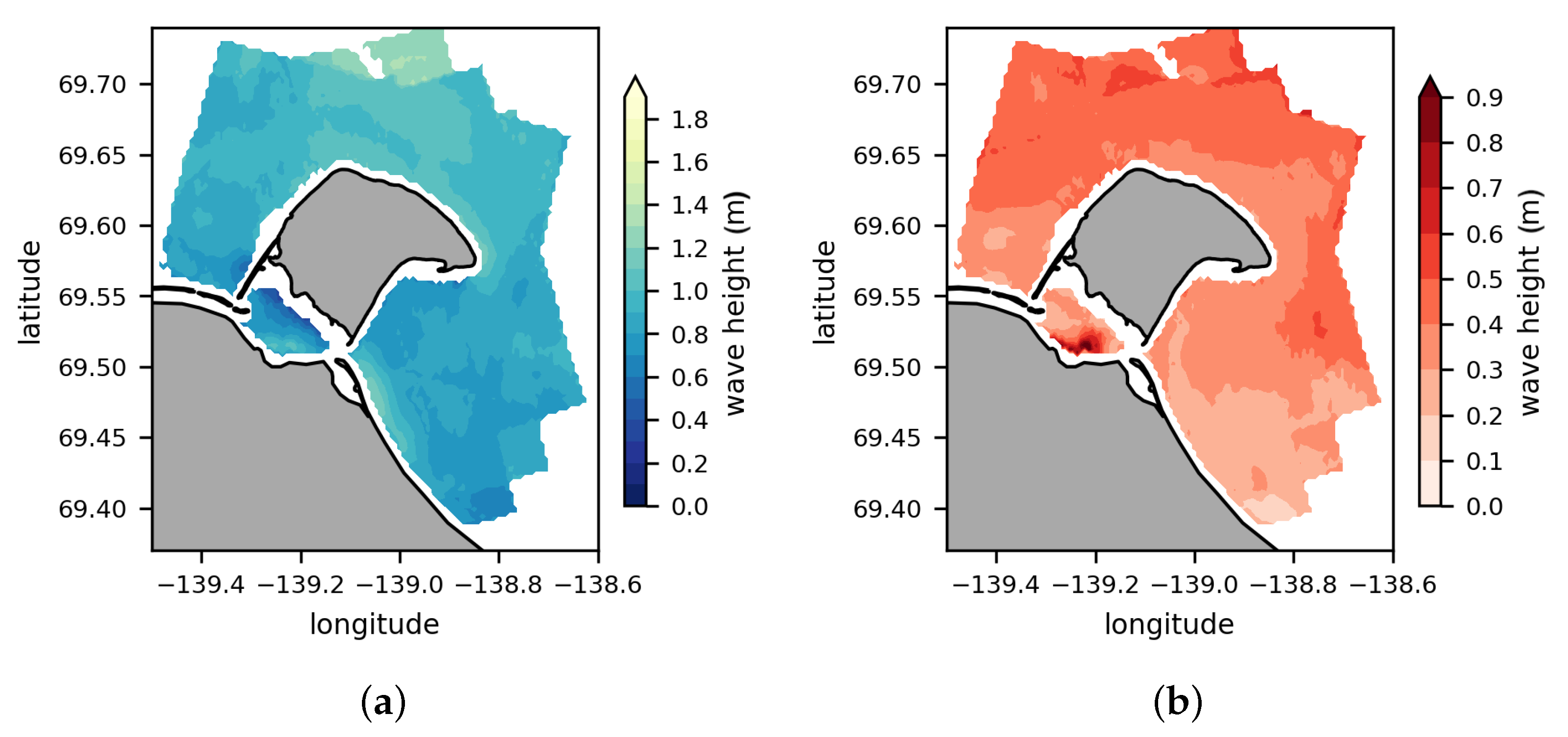
19] but are limited by their cell spacing of approximately 5.20 km. In contrast, the CWAVE_EX algorithm resolves significant wave heights with an original grid spacing of about 600 m. An analysis of the spatial wave patterns reveals distinct wave height distributions (Figure 8) not previously reported in the literature for Arctic nearshore environments. It highlights the importance of considering the spatial distribution of wave heights when trying to project the evolution of the changing Arctic coastline.
Our results suggest a clear seasonal gradient which is consistent with the existing studies. Wave heights increase throughout the entire study area towards October (Figure 12, Table 5). This is likely to be due to the general increase in storm activity towards October [10,44], which can also be seen in the local wind statistics (Figure A1). Ref [19] showed that mean significant wave heights increased by up to 0.60 m during the study period 1992 to 2013, while our results show an increase of about 0.40 m (considering the whole study area). ROI 6, located further offshore, shows an increase consistent with the results of [19] (Table 5).
The whole dataset of the spatial wave height patterns (Figure 8a) reflects the dominant NW and ESE wind regimes. The results show a bimodal distribution of the wave height according to the wind regimes (Figure 9). This is also shown in the spatial distribution of the standard deviations (Figure 8b), resulting in higher values where the wind regimes lead to a large variability in the H s values, as in ROI 1 (Figure 8b, Table 4). Especially in ROI 1, west of HIQ, the high variability in the wave heights between the wind regimes can be observed. During ESE winds, this ROI is on the lee side of HIQ and therefore experiences less wind stress, resulting in lower wave heights. The opposite occurs during NW winds. When the ROI is on the windward side, the wind transfers energy to the water surface, allowing waves to potentially fully develop [17].
Furthermore, the bimodal spatial patterns between the wind regimes may indicate the fetch-limited growth of wind-induced waves, as shown by several observational studies (e.g., [74,75,76]). The waves seen in ROI 2 and ROI 6 can develop over long distances during NW wind conditions. These ROIs face the offshore waters of the Beaufort Sea where fetch lengths can exceed 1000 km [10]. As a result, the mean wave heights are greater (Figure 10a) compared to the ESE conditions. For instance, the waves reaching Thetis Bay (ROI 5) are generated over a much shorter fetch (about 20 km under the ESE wind conditions).
Thetis Bay consistently reflects the lowest wave heights under all the wind regimes and months. Thereby, it is significantly different from any other ROI around the island. It is protected by HIQ during NW conditions [44] and by the Simpson Point sand spit [43]. In addition, the waves generated during ESE conditions are limited by the small fetch. Therefore, wind directions have a limited effect on wave heights in Thetis Bay (Table 4). Not surprisingly, Pauline Cove and Thetis Bay were used by the whaling industry in the late 19th to early 20th century for this very reason [77]. In fact, Pauline Cove is one of the few natural harbours along the Yukon coast [43].
In contrast to Thetis Bay, the northernmost point of HIQ (ROI 2), Bell Bluff (ROI 3) and Collinson Head (ROI 4) experience relatively high waves in all wind regimes and months. This can be explained by the long fetch length over the Beaufort Sea but also by the coastal morphology and hydrodynamic conditions. Collinson Head is exposed to wind stress during the ESE and NW wind regimes, while Bell Bluff and ROI 2 are only directly exposed during ESE conditions. However, the radar images during ESE conditions indicate diffraction effects at Collinson Head (Figure 14) with a leeward change in the wave propagation [78]. Thus, the wave energy is still high when entering the shadow area [79] (e.g., ROI 2). Easterly wind conditions would further lead to wave refraction at Collinson Head due to decreasing water depths [80,81] as shown in Figure 15.
Spatial wave patterns can be directly related to coastal erosion rates. Ref. [47] studied erosion rates around HIQ and concluded that the highest erosion rates are found along the NE shoreline and around Collinson Head. In contrast, much lower rates occur within Thetis Bay and on the west coast. This work can support their results. The areas with the highest erosion rates are ROIs with the highest significant wave heights (ROI 2, ROI 3 and ROI 4) as shown in Figure 8a and Table 3. These ROIs are exposed to higher waves than, e.g., Thetis Bay (Figure 9) in all the wind regimes. Particularly during NW storm events, this can result in exceptionally high erosion rates due to block failure or other types of mass movement [82]. The west coast (ROI 1) has lower volumetric erosion rates, which could be a result of its relatively sheltered position during ESE events as shown in Figure 9.
The results of this work suggest that the distance to shore does not influence the wave height north of HIQ. Based on the rank-sum test method, no significant differences occur between ROI 6 and ROIs 2 and 3 throughout the dataset. The distribution of the wave heights is similar and can be considered as deep-water wave heights according to [83]. Ref. [83] showed that deep-water wave height distribution models perform best with relative wave heights H r < 0.2 m. All three ROIs meet this threshold with mean water depths greater than 20 m and relative wave heights H r between 0.03 m and 0.05 m (Table 6). The opposite is true for Catton Point with ROI 7. Here, the relative wave height of 0.23 is very high compared to the other ROIs. This ROI is located in an area with relatively low water depths of around 4.57 m (Table 6, Figure 15). The generally high wave heights throughout the dataset may be due to an unwanted imaging effect of toppling waves [67].
In the vicinity of HIQ, waves can potentially transport suspended sediment offshore. In general, waves and wave-driven currents can contribute to the offshore mobilisation of material derived from collapsed coastal permafrost features [20]. According to [84], onshore-to-offshore sediment transport can be described as a direct function of significant wave heights. In this case, H s must be equal to or greater than 1 m to determine the sediment path offshore. On the northern side of the island, ROI 2 and ROI 6 have mean wave heights above 1 m, and therefore offshore surface sediment transport is generally possible. This assumption is supported by the results of [45]. Ref. [45] used optical satellite imagery to evaluate the distribution of the suspended sediment around HIQ by wind direction. Offshore transport can be detected with about 25 FNU up to 50 FNU in all wind directions. However, Ref. [45] indicates that offshore transport is most pronounced during ESE wind conditions north of the island. For the same wind direction, the SAR wave height calculations show mean H s values below 1 m in the northern ROIs (ROI 2 and ROI 3) (Table 4). Yet the standard deviation of 0.31 to 0.35 m indicates that an H s greater than 1 m occurs. The calculated wave heights would further suggest that higher sediment transport offshore is possible under the NW wind regime, although this assumption is not consistent with the results of [45]. However, [45] note that under ESE conditions, the background turbidity is generally higher due to the Mackenzie sediment plume east of HIQ and may therefore be decoupled from the local wave patterns.
Sediment transport along the coast around HIQ [45] may also be influenced by significant wave heights. Longshore sediment transport depends on wave characteristics, such as the significant wave height at breaking, water depth at breakpoint, breaker index and breaker angle [85]. The area around Catton Point has large H s values in all the regimes, through which large wave energy can reach the shore if it is not dissipated first. In particular, under the ESE wind regime, ROI 7 reaches the highest H s values compared to the other ROIs, which coincides with high suspended sediment concentrations [45] and longshore sediment drift [51]. However, there is a possibility that the low water depths in ROI 7 led to an overestimation of the wave heights by the CWAVE_EX algorithm [67].
The CWAVE_EX algorithm is based on high-resolution SAR imagery. It is a major improvement over many large-scale re-analysis models. The unique combination of different SAR features with image spectra and several control sequences incorporated in the SSP allows the investigation of local variations in significant wave heights. However, it is limited by the influence of land on the wave spectra and by the chaotic conditions associated with breaking waves at the shore, which reduce the imaging accuracy. With the 600 m buffer zone used in this study, it is not possible to resolve the wave climate closer to the shore. Yet this would be of great interest in processing wave impacts on the shoreline.
In situ measurements of wave heights around HIQ are scarce. Nevertheless, a comparison with previous in situ measurements shows that our results are in the same range of significant wave heights. Ref. [58] measured the wave heights on the inner Beaufort Shelf and concluded that the heights rarely exceeded 1.20 m, similar to the CWAVE_EX wave heights. Another study near King Point (about 40 km southeast of HIQ) showed wave heights of up to 0.80 m [44]. Between August 4th and 18th, the wave heights were measured near Catton Point [86], close to HIQ. During this period, the wave heights did not exceed 0.49 m, which is consistent with the relatively low wave heights around the island.

5. Conclusions

The aim of this study was to investigate the spatial variability of H s in the nearshore waters around HIQ over several years using the empirical CWAVE_EX algorithm. For this purpose, the entire ice-free TS-X/TD-X archive covering HIQ was considered. In total, 175 high-resolution H s scenes acquired between 2009 and 2020 were generated and analysed under different variables, i.e., wind regime and month.
The results show clear spatial patterns for the two dominant wind regimes, ESE and NW. Furthermore, a strong seasonal gradient can be observed, culminating in higher waves in October. The spatial patterns observed in our study reflect the traditional use of the island as a safe harbour by the Inuvialuit and explain some of the high erosion rates observed on the exposed sections of the coastline.
This approach has great potential to resolve processes at a local scale that are not covered by currently used re-analysis and wave hindcasts. Mapping significant wave heights can fill an important gap in understanding the spatial link between environmental forcing on erosion processes, suspended sediment transport, wave-driven current systems and for safe navigation along the shore. It is the first study of its kind in an Arctic environment, where data on waves and currents are otherwise scarce.
The emergence of new SAR platforms, such as Sentinel-1, will contribute to the sheer amount of data required to make this approach better suited to local environments. Yet its operationalisation would require added capacity in in situ wave monitoring. However, wave monitoring in the Arctic is in its infancy and very few stations or sensors are being deployed along the Arctic rim. This is detrimental to the development of remote sensing approaches, which rely on field observation to validate their outputs.

Supplementary Materials

The following supporting information can be downloaded at: https://www.mdpi.com/article/10.3390/rs15194753/s1.

Author Contributions

Conceptualisation, K.B. and H.L.; data curation, K.B. and A.P.; formal analysis, K.B.; investigation, K.B.; methodology, K.B., A.P. and H.L.; software, K.B. and A.P.; supervision, H.L.; visualisation, K.B.; writing—original draft, K.B. All authors have read and agreed to the published version of the manuscript.

Funding

The research leading to this study received support from the Nunataryuk project, funded by the European Union’s Horizon 2020 Research and Innovation Program under grant agreement No. 773421. We acknowledge the support of Deutsche Forschungsgemeinschaft (German Research Foundation) and the Open Access Publication Fund of the University of Potsdam.

Data Availability Statement

https://zenodo.org/ (accessed on 27 September 2023). The data used in this study is available on ZENODO: https://zenodo.org/ (accessed on 27 September 2023). The doi of the data is: https://doi.org/10.5281/zenodo.8222128 (accessed on 27 September 2023).

Acknowledgments

We would like to thank A. Roth (DLR) for supporting us in acquiring the TerraSAR-X and TanDEM-X imagery. We would like to thank J. Gimsa and K. Klein for their help during the statistical analysis and for supporting us in acquiring local weather data.

Conflicts of Interest

The authors declare no conflict of interest.

Abbreviations

The following abbreviations are used in this manuscript:
GLCMGrey-Level Co-Occurrence Matrix
HIQHerschel Island Qikiqtaruk
H s Significant Wave Height
MGDMulti-Look Ground Range Detected
NRCSNormalised Radar Cross-Section
RERadiometrically Enhanced
ROIRegion of Interest
SARSynthetic Aperture Radar
SMStripMap
SSPSea State Processor
TD-XTanDEM-X
TS-XTerraSAR-X

Appendix A

Table A1. List of TS-X and TD-X scenes used in this study. The data were acquired from the EOWEB GeoPortal: https://eoweb.dlr.de/egp/ (accessed on 27 September 2023).
DateMissionPassPolarisationLatitudeLongitude
2009-07-25TS-Xdesc.HH69.6044−139.0808
2009-08-05TS-Xdesc.HH69.6043−139.0875
2009-08-16TS-Xdesc.HH69.6049−139.0825
2009-08-27TS-Xdesc.HH69.6043−139.0794
2010-07-01TS-Xdesc.HH69.6043−139.0808
2010-07-10TS-Xasc.HH69.5906−139.0511
2010-07-12TS-Xdesc.HH69.6037−139.0831
2010-07-21TS-Xasc.HH69.5905−139.0540
2010-07-23TS-Xdesc.HH69.6039−139.0796
2010-08-01TS-Xasc.HH69.5903−139.0539
2010-08-03TS-Xdesc.HH69.6031−139.0751
2010-08-12TS-Xasc.HH69.5911−139.0497
2010-08-23TS-Xasc.HH69.5897−139.0537
2010-08-25TS-Xdesc.HH69.6038−139.0820
2010-09-03TS-Xasc.HH69.5902−139.0555
2010-09-05TS-Xdesc.HH69.6052−139.0752
2010-09-14TS-Xasc.HH69.5888−139.0572
2010-09-27TS-Xdesc.HH69.6042−139.0774
2010-10-06TD-Xasc.HH69.5909−139.0565
2011-07-07TS-Xasc.HH VV69.2641−138.7534
2011-07-21TS-Xdesc.HH HV69.3456−138.7923
2011-07-22TS-Xdesc.HH HV69.5764−139.1487
2011-07-24TS-Xasc.HH HV69.5958−139.0927
2011-09-03TS-Xdesc.HH VV69.4949−139.6426
2011-09-14TS-Xdesc.HH VV69.5269−139.2939
2011-09-25TS-Xdesc.HH VV69.4681−139.0229
2013-07-16TS-Xdesc.HH VV69.4955−139.6424
2013-07-18TS-Xasc.HH69.5896−139.0330
2013-09-09TS-Xdesc.HH VV69.5277−139.2940
2013-09-11TD-Xasc.HH69.5895−139.0291
2013-10-14TD-Xasc.HH69.5901−139.0315
2015-07-06TS-Xdesc.HH VV69.5476−139.1426
2015-07-07TS-Xdesc.VH VV69.5321−139.0839
2015-07-09TS-Xasc.HH VV69.5719−138.9514
2015-07-10TD-Xasc.HH VV69.5763−138.8736
2015-07-12TS-Xdesc.HH VV69.4675−139.0211
2015-07-15TS-Xasc.VH VV69.5363−139.0317
2015-07-17TS-Xdesc.HH VV69.5484−139.1455
2015-07-18TS-Xdesc.VH VV69.5325−139.0853
2015-07-20TS-Xasc.HH VV69.5723−138.9503
2015-07-21TS-Xasc.HH VV69.5767−138.8773
2015-07-26TS-Xasc.VH VV69.5364−139.0357
2015-07-28TS-Xdesc.HH VV69.5467−139.1450
2015-07-29TS-Xdesc.VH VV69.5316−139.0842
2015-08-03TS-Xdesc.HH VV69.4671−139.0189
2015-08-06TS-Xasc.VH VV69.5358−139.0337
2015-08-11TS-Xasc.HH VV69.5713−138.9479
2015-08-14TS-Xdesc.HH VV69.4679−139.0242
2015-08-17TD-Xasc.VH VV69.5365−139.0309
2015-09-05TS-Xdesc.HH VV69.4674−139.0201
2015-09-08TS-Xasc.VH VV69.5364−139.0344
2015-09-10TS-Xdesc.HH VV69.5472−139.1448
2015-09-11TS-Xdesc.VH VV69.5323−139.0840
2015-09-13TS-Xasc.HH VV69.5721−138.9495
2015-09-14TS-Xasc.HH VV69.5767−138.8756
2015-09-16TS-Xdesc.HH VV69.4666−139.0218
2015-09-19TS-Xasc.VH VV69.5360−139.0361
2015-09-21TS-Xdesc.HH VV69.5471−139.1410
2015-09-24TS-Xasc.HH VV69.5718−138.9507
2015-09-25TS-Xasc.HH VV69.5763−138.8779
2015-09-27TS-Xdesc.HH VV69.4675−139.0221
2015-09-30TS-Xasc.VH VV69.5363−139.0336
2015-10-02TS-Xdesc.HH VV69.5470−139.1437
2016-06-14TS-Xasc.HH VV69.5707−138.9499
2016-06-15TS-Xasc.HH VV69.5761−138.8766
2016-06-17TS-Xdesc.HH VV69.4679−139.0229
2016-06-20TS-Xasc.VH VV69.5362−139.0323
2016-06-22TS-Xdesc.HH VV69.5470−139.1461
2016-06-23TS-Xdesc.VH VV69.5323−139.0860
2016-06-25TS-Xasc.HH VV69.5715−138.9504
2016-06-26TS-Xasc.HH VV69.5750−138.8781
2016-06-28TS-Xdesc.HH VV69.4674−139.0217
2016-07-01TS-Xasc.VH VV69.5356−139.0344
2016-07-03TS-Xdesc.HH VV69.5479−139.1471
2016-07-06TS-Xasc.HH VV69.5720−138.9481
2016-07-07TS-Xasc.HH VV69.5766−138.8767
2016-07-09TS-Xdesc.HH VV69.4677−139.0216
2016-07-12TS-Xasc.VH VV69.5362−139.0346
2016-07-17TS-Xasc.HH VV69.5725−138.9481
2016-07-18TD-Xasc.HH VV69.5767−138.8736
2016-07-20TS-Xdesc.HH VV69.4673−139.0229
2016-07-23TS-Xasc.VH VV69.5361−139.0347
2016-07-25TS-Xdesc.HH VV69.5473−139.1427
2016-07-28TS-Xasc.HH VV69.5718−138.9513
2016-07-29TS-Xasc.HH VV69.5766−138.8785
2016-07-31TS-Xdesc.HH VV69.4664−139.0214
2016-08-03TS-Xasc.VH VV69.5352−139.0330
2016-08-05TS-Xdesc.HH VV69.5474−139.1428
2016-08-06TS-Xdesc.VH VV69.5319−139.0827
2016-08-08TD-Xasc.HH VV69.5718−138.9525
2016-08-09TD-Xasc.HH VV69.5760−138.8804
2016-08-11TS-Xdesc.HH VV69.4673−139.0184
2016-08-14TD-Xasc.VH VV69.5358−139.0357
2016-08-16TS-Xdesc.HH VV69.5477−139.1418
2016-08-20TS-Xasc.HH VV69.5760−138.8811
2016-08-22TS-Xdesc.HH VV69.4668−139.0192
2016-08-25TS-Xasc.VH VV69.5357−139.0371
2016-08-27TS-Xdesc.HH VV69.5471−139.1421
2016-08-30TD-Xasc.HH VV69.5723−138.9505
2016-08-31TD-Xasc.HH VV69.5767−138.8786
2016-09-02TS-Xdesc.HH VV69.4678−139.0217
2016-09-05TD-Xasc.VH VV69.5361−139.0363
2016-09-07TS-Xdesc.HH VV69.5474−139.1410
2016-09-10TD-Xasc.HH VV69.5715−138.9551
2016-09-11TD-Xasc.HH VV69.5760−138.8800
2016-09-13TS-Xdesc.HH VV69.4677−139.0204
2016-09-16TS-Xasc.VH VV69.5358−139.0336
2016-09-18TS-Xdesc.HH VV69.5469−139.1439
2016-09-19TS-Xdesc.VH VV69.5319−139.0831
2016-09-22TS-Xasc.HH VV69.5763−138.8828
2016-09-24TS-Xdesc.HH VV69.4672−139.0181
2016-09-29TS-Xdesc.HH VV69.5465−139.1435
2016-09-30TS-Xdesc.VH VV69.5314−139.0830
2016-10-03TS-Xasc.HH VV69.5766−138.8780
2016-10-05TS-Xdesc.HH VV69.4670−139.0201
2016-10-08TS-Xasc.VH VV69.5362−139.0397
2017-06-29TD-Xasc.VH VV69.5366−139.0315
2017-07-05TD-Xasc.HH VV69.5764−138.8725
2017-07-07TS-Xdesc.HH VV69.4686−139.0287
2017-07-10TS-Xasc.VH VV69.5370−139.0283
2017-07-16TS-Xasc.HH VV69.5769−138.8741
2017-07-18TS-Xdesc.HH VV69.4681−139.0227
2017-07-21TS-Xasc.VH VV69.5360−139.0304
2017-07-27TS-Xasc.HH VV69.5763−138.8729
2017-07-29TS-Xdesc.HH VV69.4671−139.0240
2017-08-07TS-Xasc.HH VV69.5777−138.8723
2017-08-09TS-Xdesc.HH VV69.4673−139.0249
2017-08-12TS-Xasc.VH VV69.5360−139.0295
2017-08-18TS-Xasc.HH VV69.5765−138.8711
2017-08-20TS-Xdesc.HH VV69.4675−139.0258
2017-08-31TS-Xdesc.HH VV69.4686−139.0241
2017-09-03TS-Xasc.VH VV69.5365−139.0314
2017-09-09TS-Xasc.HH VV69.5766−138.8731
2017-09-11TS-Xdesc.HH VV69.4680−139.0249
2017-09-14TS-Xasc.VH VV69.5357−139.0350
2017-09-25TD-Xasc.VH VV69.5365−139.0310
2017-09-28TD-Xdesc.VH VV69.5309−139.0780
2017-10-03TD-Xdesc.HH VV69.4673−139.0263
2017-10-09TD-Xdesc.VH VV69.5319−139.0782
2017-10-12TD-Xasc.HH VV69.5768−138.8758
2017-10-14TS-Xdesc.HH VV69.4670−139.0169
2017-10-17TD-Xasc.VH VV69.5365−139.0316
2018-09-18TD-Xasc.HH VV69.5771−138.8796
2018-09-29TD-Xasc.HH VV69.5766−138.8784
2018-10-10TD-Xasc.HH VV69.5761−138.8787
2019-06-22TD-Xdesc.HH VV69.3971−139.0761
2019-06-25TD-Xasc.VH VV69.5350−139.0335
2019-06-28TS-Xdesc.HH VV69.5322−139.0850
2019-07-03TS-Xdesc.HH VV69.3984−139.0782
2019-07-06TD-Xasc.VH VV69.5356−139.0327
2019-07-09TS-Xdesc.HH VV69.5322−139.0835
2019-07-17TS-Xasc.VH VV69.5365−139.0308
2019-07-28TS-Xasc.VH VV69.5360−139.0348
2019-07-31TS-Xdesc.HH VV69.5314−139.0872
2019-08-05TS-Xdesc.HH VV69.3968−139.0741
2019-08-08TS-Xasc.VH VV69.5356−139.0368
2019-08-19TD-Xasc.VH VV69.5361−139.0299
2019-08-27TD-Xdesc.HH VV69.3976−139.0768
2019-09-13TD-Xdesc.HH VV69.4391−139.1378
2019-09-16TD-Xasc.HH VV69.5775−138.8754
2019-09-18TS-Xdesc.HH VV69.3967−139.0749
2019-09-21TD-Xasc.VH VV69.5360−139.0341
2019-10-02TD-Xasc.VH VV69.5361−139.0350
2019-10-05TD-Xdesc.HH VV69.4379−139.1304
2019-10-08TD-Xasc.HH VV69.5759−138.8807
2019-10-10TS-Xdesc.HH VV69.3973−139.0705
2019-10-13TD-Xasc.VH VV69.5358−139.0367
2019-10-24TD-Xasc.VH VV69.5359−139.0390
2020-07-03TD-Xasc.VH VV69.5355−139.0300
2020-07-09TD-Xasc.HH VV69.5770−138.8717
2020-07-11TS-Xdesc.HH VV69.3975−139.0771
2020-07-14TD-Xasc.VH VV69.5362−139.0314
2020-08-05TD-Xasc.VH VV69.5359−139.0315
2020-08-24TS-Xdesc.HH VV69.3972−139.0743
2020-09-13TD-Xasc.HH VV69.5764−138.8780
Table A2. Normalised frequency in descending order of different footprints measured by orbit number within the dataset and the associated satellite pass, either descending (desc.) or ascending (asc.).
Relative Orbit NumberFrequency (%)Satellite Pass
6124.59asc.
2423.50desc.
15218.03asc.
11512.02desc.
10010.38desc.
1379.29asc.
462.19asc.
Figure A1. Wind rose diagram with wind speed and wind direction for each month during the open-water season. Data were acquired over the years 2009 to 2020 from the weather station at Simpson Point on HIQ [71]. The polar axis describes the normalised frequency of wind direction.
Remotesensing 15 04753 g0a1

References

  1. IPCC. The Physical Science Basis. In Contribution of Working Group I to the Sixth Assessment Report of the Intergovernmental Panel on Climate Change; Cambridge University Press: Cambridge, UK, 2007. [Google Scholar]
  2. Stroeve, J.; Holland, M.M.; Meier, W.; Scambos, T.; Serreze, M. Arctic sea ice decline: Faster than forecast. Geophys. Res. Lett. 2007, 34, 3498. [Google Scholar] [CrossRef]
  3. Stroeve, J.C.; Kattsov, V.; Barrett, A.; Serreze, M.; Pavlova, T.; Holland, M.; Meier, W.N. Trends in Arctic sea ice extent from CMIP5, CMIP3 and observations. Geophys. Res. Lett. 2012, 39. [Google Scholar] [CrossRef]
  4. Stroeve, J.C.; Serreze, M.C.; Holland, M.M.; Kay, J.E.; Malanik, J.; Barrett, A.P. The Arctic’s rapidly shrinking sea ice cover: A research synthesis. Clim. Chang. 2012, 110, 1005–1027. [Google Scholar] [CrossRef]
  5. Walsh, J.E. Intensified warming of the Arctic: Causes and impacts on middle latitudes. Glob. Planet. Chang. 2014, 117, 52–63. [Google Scholar] [CrossRef]
  6. Notz, D.; Community, S. Arctic Sea Ice in CMIP6. Geophys. Res. Lett. 2020, 47, e2019GL086749. [Google Scholar] [CrossRef]
  7. Mioduszewski, J.; Vavrus, S.; Wang, M. Diminishing Arctic Sea Ice Promotes Stronger Surface Winds. J. Clim. 2018, 31, 8101–8119. [Google Scholar] [CrossRef]
  8. Rinke, A.; Maturilli, M.; Graham, R.M.; Matthes, H.; Handorf, D.; Cohen, L.; Hudson, S.R.; Moore, J.C. Extreme cyclone events in the Arctic: Wintertime variability and trends. Environ. Res. Lett. 2017, 12, 094006. [Google Scholar] [CrossRef]
  9. Zhang, X.; Walsh, J.E.; Zhang, J.; Bhatt, U.S.; Ikeda, M. Climatology and Interannual Variability of Arctic Cyclone Activity: 1948–2002. J. Clim. 2004, 17, 2300–2317. [Google Scholar] [CrossRef]
  10. Atkinson, D.E. Observed storminess patterns and trends in the circum-Arctic coastal regime. Geo-Mar. Lett. 2005, 25, 98–109. [Google Scholar] [CrossRef]
  11. Overeem, I.; Anderson, R.S.; Wobus, C.W.; Clow, G.D.; Urban, F.E.; Matell, N. Sea ice loss enhances wave action at the Arctic coast. Geophys. Res. Lett. 2011, 38, 17. [Google Scholar] [CrossRef]
  12. Stopa, J.E.; Ardhuin, F.; Girard-Ardhuin, F. Wave climate in the Arctic 1992–2014: Seasonality and trends. Cryosphere 2016, 10, 1605–1629. [Google Scholar] [CrossRef]
  13. Barnhart, K.R.; Overeem, I.; Anderson, R.S. The effect of changing sea ice on the physical vulnerability of Arctic coasts. Cryosphere 2014, 8, 1777–1799. [Google Scholar] [CrossRef]
  14. Semedo, A.; Vettor, R.; Breivik, Ø.; Sterl, A.; Reistad, M.; Soares, C.G.; Lima, D. The wind sea and swell waves climate in the Nordic seas. Ocean Dyn. 2015, 65, 223–240. [Google Scholar] [CrossRef]
  15. Waseda, T.; Webb, A.; Sato, K.; Inoue, J.; Kohout, A.; Penrose, B.; Penrose, S. Correlated Increase of High Ocean Waves and Winds in the Ice-Free Waters of the Arctic Ocean. Sci. Rep. 2018, 8, 4489. [Google Scholar] [CrossRef]
  16. Liu, Q.; Babanin, A.V.; Zieger, S.; Young, I.R.; Guan, C. Wind and Wave Climate in the Arctic Ocean as Observed by Altimeters. J. Clim. 2016, 29, 7957–7975. [Google Scholar] [CrossRef]
  17. Thomson, J.; Rogers, W.E. Swell and sea in the emerging Arctic Ocean. Geophys. Res. Lett. 2014, 41, 3136–3140. [Google Scholar] [CrossRef]
  18. Thomson, J.; Fan, Y.; Stammerjohn, S.; Stopa, J.; Rogers, W.E.; Girard-Ardhuin, F.; Ardhuin, F.; Shen, H.; Perrie, W.; Shen, H.; et al. Emerging trends in the sea state of the Beaufort and Chukchi seas. Ocean Model. 2016, 105, 1–12. [Google Scholar] [CrossRef]
  19. Wang, X.L.; Feng, Y.; Swail, V.R.; Cox, A. Historical Changes in the Beaufort–Chukchi–Bering Seas Surface Winds and Waves, 1971–2013. J. Clim. 2015, 28, 7457–7469. [Google Scholar] [CrossRef]
  20. Aré, F.E. Thermal abrasion of sea coasts (part I). Polar Geogr. Geol. 1988, 12, 1. [Google Scholar] [CrossRef]
  21. Jones, B.M.; Arp, C.D.; Jorgenson, M.T.; Hinkel, K.M.; Schmutz, J.A.; Flint, P.L. Increase in the rate and uniformity of coastline erosion in Arctic Alaska. Geophys. Res. Lett. 2009, 36, 3. [Google Scholar] [CrossRef]
  22. Lantuit, H.; Overduin, P.P.; Couture, N.; Wetterich, S.; Aré, F.; Atkinson, D.; Brown, J.; Cherkashov, G.; Drozdov, D.; Forbes, D.L.; et al. The Arctic Coastal Dynamics Database: A New Classification Scheme and Statistics on Arctic Permafrost Coastlines. Estuaries Coasts 2012, 35, 383–400. [Google Scholar] [CrossRef]
  23. Solomon, S.M. Spatial and temporal variability of shoreline change in the Beaufort-Mackenzie region, northwest territories, Canada. Geo-Mar. Lett. 2005, 25, 127–137. [Google Scholar] [CrossRef]
  24. Günther, F.; Overduin, P.P.; Yakshina, I.A.; Opel, T.; Baranskaya, A.V.; Grigoriev, M.N. Observing Muostakh disappear: Permafrost thaw subsidence and erosion of a ground-ice-rich island in response to arctic summer warming and sea ice reduction. Cryosphere 2015, 9, 151–178. [Google Scholar] [CrossRef]
  25. Nielsen, D.M.; Pieper, P.; Barkhordarian, A.; Overduin, P.; Ilyina, T.; Brovkin, V.; Baehr, J.; Dobrynin, M. Increase in Arctic coastal erosion and its sensitivity to warming in the twenty-first century. Nat. Clim. Chang. 2022, 12, 1. [Google Scholar] [CrossRef]
  26. Carmack, E.; Wassmann, P. Food webs and physical–biological coupling on pan-Arctic shelves: Unifying concepts and comprehensive perspectives. Prog. Oceanogr. 2006, 71, 446–477. [Google Scholar] [CrossRef]
  27. Wegner, C.; Holdemann, J.; Dmitrenko, I.; Kirillov, S.; Kassens, H. Seasonal variations in Arctic sediment dynamics—evidence from 1-year records in the Laptev Sea (Siberian Arctic). Glob. Planet. Chang. 2005, 48, 126–140. [Google Scholar] [CrossRef]
  28. Lemmen, D.S.; Warren, F.J.; James, T.S.; Clarke, C.S.L.M. (Eds.) Canada’s Marine Coasts in a Changing Climate; Government of Canada = Gouvernement du Canada: Ottawa, ON, Canada, 2016. [Google Scholar]
  29. Grifoll, M.; Martínez de Osés, F.X.; Castells, M. Potential economic benefits of using a weather ship routing system at Short Sea Shipping. WMU J. Marit. Aff. 2018, 17, 195–211. [Google Scholar] [CrossRef]
  30. Héquette, A.; Jenner, K.A.; Hill, P.R. Beach Morphodynamics and Sediment Transport at Tibjak Beach, Canadian Beaufort Sea Coast; Geological Survey of Canada: Ottawa, ON, Canada, 1990.
  31. Breit, H.; Fritz, T.; Balss, U.; Lachaise, M.; Niedermeier, A.; Vonavka, M. TerraSAR-X SAR Processing and Products. IEEE Trans. Geosci. Remote Sens. 2010, 48, 727–740. [Google Scholar] [CrossRef]
  32. Schulz-Stellenfleth, J.; König, T.; Lehner, S. An empirical approach for the retrieval of integral ocean wave parameters from synthetic aperture radar data. J. Geophys. Res. 2007, 112, 12613. [Google Scholar] [CrossRef]
  33. Stopa, J.E.; Mouche, A. Significant wave heights from Sentinel-1 SAR: Validation and applications. J. Geophys. Res. Oceans 2017, 122, 1827–1848. [Google Scholar] [CrossRef]
  34. Pleskachevsky, A.; Jacobsen, S.; Tings, B.; Schwarz, E. Estimation of sea state from Sentinel-1 Synthetic aperture radar imagery for maritime situation awareness. Int. J. Remote Sens. 2019, 40, 4104–4142. [Google Scholar] [CrossRef]
  35. Bruck, M. Sea State Measurements using TerraSAR-X/TanDEM-X Data. Ph.D. Thesis, Christian-Albrechts-Universität zu Kiel, Kiel, Germany, 2015. [Google Scholar]
  36. Gao, D.; Liu, Y.; Meng, J.; Jia, Y.; Fan, C. Estimating significant wave height from SAR imagery based on an SVM regression model. Acta Oceanol. Sin. 2018, 37, 103–110. [Google Scholar] [CrossRef]
  37. Kumar, N.K.; Savitha, R.; Al Mamun, A. Ocean wave height prediction using ensemble of Extreme Learning Machine. Neurocomputing 2018, 277, 12–20. [Google Scholar] [CrossRef]
  38. Shao, W.; Ding, Y.; Li, J.; Gou, S.; Nunziata, F.; Yuan, X.; Zhao, L. Wave Retrieval Under Typhoon Conditions Using a Machine Learning Method Applied to Gaofen-3 SAR Imagery. Can. J. Remote Sens. 2019, 45, 723–732. [Google Scholar] [CrossRef]
  39. Wu, K.; Li, X.M.; Huang, B. Retrieval of Ocean Wave Heights From Spaceborne SAR in the Arctic Ocean With a Neural Network. J. Geophys. Res. Oceans 2021, 126, e2020JC016946. [Google Scholar] [CrossRef]
  40. Wang, H.; Yang, J.; Lin, M.; Li, W.; Zhu, J.; Ren, L.; Cui, L. Quad-polarimetric SAR sea state retrieval algorithm from Chinese Gaofen-3 wave mode imagettes via deep learning. Remote Sens. Environ. 2022, 273, 112969. [Google Scholar] [CrossRef]
  41. Quach, B.; Glaser, Y.; Stopa, J.E.; Mouche, A.A.; Sadowski, P. Deep Learning for Predicting Significant Wave Height From Synthetic Aperture Radar. IEEE Trans. Geosci. Remote Sens. 2021, 59, 1859–1867. [Google Scholar] [CrossRef]
  42. Pleskachevsky, A.; Tings, B.; Wiehle, S.; Imber, J.; Jacobsen, S. Multiparametric sea state fields from synthetic aperture radar for maritime situational awareness. Remote Sens. Environ. 2022, 280, 113200. [Google Scholar] [CrossRef]
  43. Burn, C.R.; Zhang, Y. Permafrost and climate change at Herschel Island (Qikiqtaruq), Yukon Territory, Canada. J. Geophys. Res. 2009, 114, 546. [Google Scholar] [CrossRef]
  44. Hill, P.R.; Blasco, S.M.; Harper, J.R.; Fissel, D.B. Sedimentation on the Canadian Beaufort Shelf. Cont. Shelf Res. 1991, 11, 821–842. [Google Scholar] [CrossRef]
  45. Klein, K.P.; Lantuit, H.; Heim, B.; Fell, F.; Doxaran, D.; Irrgang, A.M. Long-Term High-Resolution Sediment and Sea Surface Temperature Spatial Patterns in Arctic Nearshore Waters Retrieved Using 30-Year Landsat Archive Imagery. Remote Sens. 2019, 11, 2791. [Google Scholar] [CrossRef]
  46. Lantuit, H.; Pollard, W.H. Fifty years of coastal erosion and retrogressive thaw slump activity on Herschel Island, southern Beaufort Sea, Yukon Territory, Canada. Geomorphology 2008, 95, 84–102. [Google Scholar] [CrossRef]
  47. Obu, J.; Lantuit, H.; Fritz, M.; Pollard, W.H.; Sachs, T.; Günther, F. Relation between planimetric and volumetric measurements of permafrost coast erosion: A case study from Herschel Island, western Canadian Arctic. Polar Res. 2016, 35, 30313. [Google Scholar] [CrossRef]
  48. Radosavljevic, B.; Lantuit, H.; Pollard, W.; Overduin, P.; Couture, N.; Sachs, T.; Helm, V.; Fritz, M. Erosion and Flooding—Threats to Coastal Infrastructure in the Arctic: A Case Study from Herschel Island, Yukon Territory, Canada. Estuaries Coasts 2016, 39, 900–915. [Google Scholar] [CrossRef]
  49. Olynyk, D.M. Summary of the significance of and threats to cultural resources located at the historic settlement area on Herschel Island territorial park of Yukon. In Heritage at Risk: ICOMOS World Report 2006/2007 on Monuments and Sites in Danger; Petzet, M., Ziesemer, J., Eds.; E. Reinhold: Altenburg, Germany, 2008; pp. 212–214. [Google Scholar]
  50. Mackay, J.R. Glacier ice-thrust features of the Yukon coast. Geogr. Bull. 1959, 13, 5–21. [Google Scholar]
  51. Pelletier, B.R.; Medioli, B.E. Environmental Atlas of the Beaufort Coastlands; Geological Survey of Canada Open File 7619; Natural Resources Canada: Ottawa, ON, Canada, 2014. [CrossRef]
  52. Burn, C.R.; Hattendorf, J.B. Place Names. In Herschel Island; Burn, C.R., Ed.; Wildlife Management Advisory Council (North Slope): Whitehorse, YT, Canada, 2012; pp. 20–27. [Google Scholar]
  53. Mulligan, R.P.; Perrie, W. Circulation and structure of the Mackenzie River plume in the coastal Arctic Ocean. Cont. Shelf Res. 2019, 177, 59–68. [Google Scholar] [CrossRef]
  54. Burn, C.R. Permafrost. In Herschel Island; Burn, C.R., Ed.; Wildlife Management Advisory Council (North Slope): Whitehorse, YT, Canada, 2012; pp. 65–71. [Google Scholar]
  55. Burn, C.R. Climate. In Herschel Island; Burn, C.R., Ed.; Wildlife Management Advisory Council (North Slope): Whitehorse, YT, Canada, 2012; pp. 48–53. [Google Scholar]
  56. Nose, T.; Webb, A.; Waseda, T.; Inoue, J.; Sato, K. Predictability of storm wave heights in the ice-free Beaufort Sea. Ocean Dyn. 2018, 68, 1383–1402. [Google Scholar] [CrossRef]
  57. Rogers, W.E.; Thomson, J.; Shen, H.H.; Doble, M.J.; Wadhams, P.; Cheng, S. Dissipation of wind waves by pancake and frazil ice in the autumn Beaufort Sea. J. Geophys. Res. Oceans 2016, 121, 7991–8007. [Google Scholar] [CrossRef]
  58. Hill, P.R.; Nadea, O.C. Storm-dominated Sedimentation on the Inner Shelf of the Canadian Beaufort Sea. SEPM J. Sediment. Res. 1989, 59, 455–468. [Google Scholar] [CrossRef]
  59. ESA. European Space Agency: Copernicus Open Access Hub. Available online: https://scihub.copernicus.eu/ (accessed on 30 August 2022).
  60. AIRBUS. TerraSAR-X Image Product Guide: Basic and Enhanced Radar Satellite Imagery. Airbus Def. Space 2015, 2, 1–24. [Google Scholar]
  61. Li, X.; Lehner, S.; Rosenthal, W. Investigation of Ocean Surface Wave Refraction Using TerraSAR-X Data. IEEE Trans. Geosci. Remote Sens. 2010, 48, 830–840. [Google Scholar] [CrossRef]
  62. Wiehle, S.; Pleskachevsky, A.; Gebhardt, C. Automatic bathymetry retrieval from SAR images. CEAS Space J. 2019, 11, 105–114. [Google Scholar] [CrossRef]
  63. Yang, Y.J.; Singha, S.; Mayerle, R. A deep learning based oil spill detector using Sentinel-1 SAR imagery. Int. J. Remote Sens. 2022, 43, 4287–4314. [Google Scholar] [CrossRef]
  64. Alpers, W.; Bruening, C. On the Relative Importance of Motion-Related Contributions to the SAR Imaging Mechanism of Ocean Surface Waves. IEEE Trans. Geosci. Remote. Sens. 1986, GE-24, 873–885. [Google Scholar] [CrossRef]
  65. Lehner, S.; Pleskachevsky, A.; Velotto, D.; Jacobsen, S. Meteo-Marine Parameters and Their Variability Observed by High Resolution Satellite Radar Images. Oceanography 2013, 26, 80–91. [Google Scholar] [CrossRef]
  66. Rikka, S.; Pleskachevsky, A.; Uiboupin, R.; Jacobsen, S. Sea state in the Baltic Sea from space-borne high-resolution synthetic aperture radar imagery. Int. J. Remote Sens. 2018, 39, 1256–1284. [Google Scholar] [CrossRef]
  67. Pleskachevsky, A.L.; Rosenthal, W.; Lehner, S. Meteo-marine parameters for highly variable environment in coastal regions from satellite radar images. ISPRS J. Photogramm. Remote Sens. 2016, 119, 464–484. [Google Scholar] [CrossRef]
  68. Li, X.M.; Lehner, S. Algorithm for Sea Surface Wind Retrieval From TerraSAR-X and TanDEM-X Data. IEEE Trans. Geosci. Remote Sens. 2014, 52, 2928–2939. [Google Scholar] [CrossRef]
  69. CMEMS. Product User Manual: For the Global Ocean Wave Multi Year Product. Available online: https://catalogue.marine.copernicus.eu/documents/PUM/CMEMS-GLO-PUM-001-032.pdf (accessed on 1 June 2023).
  70. Law-Chune, S.; Aouf, L.; Dalphinet, A.; Levier, B.; Drillet, Y.; Drevillon, M. WAVERYS: A CMEMS global wave reanalysis during the altimetry period. Ocean Dyn. 2021, 71, 357–378. [Google Scholar] [CrossRef]
  71. Government of Canada Historical Weather Data; Government of Canada: Ottawa, ON, Canada. Available online: https://climate.weather.gc.ca/historical_data/search_historic_data_e.html (accessed on 23 August 2022).
  72. Williams, B.; Carmack, E. Ocean Water and Sea Ice. In Herschel Island; Burn, C.R., Ed.; Wildlife Management Advisory Council (North Slope): Whitehorse, YT, Canada, 2012. [Google Scholar]
  73. Virtanen, P.; Gommers, R.; Oliphant, T.E.; Haberland, M.; Reddy, T.; Cournapeau, D.; Burovski, E.; Peterson, P.; Weckesser, W.; Bright, J.; et al. SciPy 1.0: Fundamental Algorithms for Scientific Computing in Python. Nat. Methods 2020, 17, 261–272. [Google Scholar] [CrossRef]
  74. Phillips, O.M. On the generation of waves by turbulent wind. J. Fluid Mech. 1957, 2, 417. [Google Scholar] [CrossRef]
  75. Romero, L.; Melville, W.K. Airborne Observations of Fetch-Limited Waves in the Gulf of Tehuantepec. J. Phys. Oceanogr. 2010, 40, 441–465. [Google Scholar] [CrossRef]
  76. Shin, Y.; Cifuentes-Lorenzen, A.; Howard Strobel, M.M.; O’Donnell, J. Waves in Western Long Island Sound: A Fetch–Limited Coastal Basin. J. Geophys. Res. Oceans 2021, 126, 224. [Google Scholar] [CrossRef]
  77. Bockstoce, J.R. Whaling. In Herschel Island; Burn, C.R., Ed.; Wildlife Management Advisory Council (North Slope): Whitehorse, YT, Canada, 2012; pp. 158–168. [Google Scholar]
  78. Burcharth, H.F.; Hawkins, S.J.; Zanuttigh, B.; Lamberti, A. Design tools related to engineering. In Environmental Design Guidelines for Low Crested Coastal Structures; Burcharth, H.F., Hawkins, S.J., Zanuttigh, B., Lamberti, A., Eds.; Elsevier: Amsterdam, The Netherlands, 2007; pp. 203–333. [Google Scholar] [CrossRef]
  79. Violante-Carvalho, N.; Arruda, W.Z.; Carvalho, L.M.; Rogers, W.E.; Passaro, M. Diffraction of irregular ocean waves measured by altimeter in the lee of islands. Remote Sens. Environ. 2021, 265, 112653. [Google Scholar] [CrossRef]
  80. Arthur, R.S. Refraction of water waves by islands and shoals with circular bottom-contours. Trans. Am. Geophys. Union 1946, 27, 168. [Google Scholar] [CrossRef]
  81. Guillou, N.; Chapalain, G. Effects of waves on the initiation of headland-associated sandbanks. Cont. Shelf Res. 2011, 31, 1202–1213. [Google Scholar] [CrossRef]
  82. Jones, B.M.; Farquharson, L.M.; Baughman, C.A.; Buzard, R.M.; Arp, C.D.; Grosse, G.; Bull, D.L.; Günther, F.; Nitze, I.; Urban, F.; et al. A decade of remotely sensed observations highlight complex processes linked to coastal permafrost bluff erosion in the Arctic. Environ. Res. Lett. 2018, 13, 115001. [Google Scholar] [CrossRef]
  83. James, J.P.; Panchang, V. Investigation of Wave Height Distributions and Characteristic Wave Periods in Coastal Environments. J. Geophys. Res. Oceans 2022, 127, 569. [Google Scholar] [CrossRef]
  84. Bailard, J.A. Modeling On-Offshore Sediment Transport in the Surfzone. In Coastal Engineering 1982; Edge, B.L., Ed.; American Society of Civil Engineers: New York, NY, USA, 1982; pp. 1419–1438. [Google Scholar] [CrossRef]
  85. Komar, P.D.; Inman, D.L. Longshore sand transport on beaches. J. Geophys. Res. 1970, 75, 5914–5927. [Google Scholar] [CrossRef]
  86. Gimsa, J. Arctic Nearshore Current Dynamics and Wave Climate under Declining Sea Ice Conditions Potential Impacts on Sediment Pathways: A Case Study From Herschel Island–Qikiqtaruk, Yukon Coast, Canada. Master’s Thesis, University of Potsdam, Postdam, Germany, 2019. [Google Scholar]
Figure 2. Flowchart of the method. Red rectangles are main inputs, yellow circles are processing steps, light blue rectangles are common outputs and dark blue rectangles are main outputs.
Remotesensing 15 04753 g002
Figure 3. Total frequency of scene footprints within the dataset, where each grid cell represents the sum of occurrences. The underlying grey area represents study area with HIQ at its centre.
Remotesensing 15 04753 g003
Figure 4. Example of processed H s with 600 m grid step using the SSP with the empirical CWAVE_EX algorithm. The two SAR images (a,b) are RE, MGD products and were acquired under different wind conditions. The wind conditions 6 h prior to the scene acquisition are represented in the wind roses in (a,b). Figure (a) was acquired under decreasing wind speeds from 10.83 m/s to 8.33 m/s, with the wind coming predominantly from the NW, producing wave heights up to 2 m. Figure (b) was acquired under increasing wind speeds from 1.11 m/s to 5.56 m/s, with the wind coming predominantly from the SE, producing wave heights generally lower than 0.46 m (third quartile).
Remotesensing 15 04753 g004
Figure 5. Comparison of TS-X/TD-X SM ice-free scenes with hindcast model results. Due to the coarser resolution of the model (about 15 km), several SAR wave height values collocated with the model grid points are visible in the vertical H s distribution.
Remotesensing 15 04753 g005
Figure 6. Wind rose diagram with wind speed and wind direction from HIQ for the years 2009 to 2020. Only data collected during the open-water season, i.e., July, August, September and October, were used.
Remotesensing 15 04753 g006
Figure 7. Location of the ROIs. ROIs 1 to 5 (black) are in close proximity to HIQ, while ROIs 6 and 7 (red) are located further away.
Remotesensing 15 04753 g007
Figure 8. Significant wave height statistics for the stacked H s -dataset (2009–2020). Figure (a) is the mean significant wave height and (b) is the standard deviation. Both parameters were calculated per grid cell.
Remotesensing 15 04753 g008
Figure 9. Mean significant wave height for the stacked Hs-dataset (2009–2020) by the dominant wind regimes calculated per grid cell. Wind directions are indicated by wind roses in the lower left corner of each plot.
Remotesensing 15 04753 g009
Figure 10. Box-plot of the Kruskal–Wallis rank-sum test of significant wave height values by (a) wind regime and (b) month. The boundaries of the rectangles indicate the 25th and 75th percentiles, and the horizontal bars indicate the median. The dashed vertical bars indicate the upper and lower limits of the distribution.
Remotesensing 15 04753 g010
Figure 11. Dunn’s test results showing the comparison of ROIs (see Figure 7) across wind regimes with a significance level of p = 0.05 . The null-hypothesis H 0 is defined as the groups are equal, where p < 0.05 rejects H 0 . Only the most frequent wind regimes are shown.
Remotesensing 15 04753 g011
Figure 12. Mean significant wave heights for the stacked Hs-dataset (2009–2020) by month, calculated per grid cell.
Remotesensing 15 04753 g012
Figure 13. Dunn’s test results showing ROI comparison over months with a significance level of p = 0.05 . The null-hypothesis H 0 is defined as the groups are equal, where p < 0.05 rejects H 0 .
Remotesensing 15 04753 g013
Figure 14. TerraSAR-X MGD RE SM HH scene from 9 July 2019 15:59:45 UTC. The scene was acquired under stable SE wind conditions.
Remotesensing 15 04753 g014
Figure 15. Interpolated bathymetry on a 300 m × 300 m grid ((Federal Publications, Inc.: Nautical charts of the Beaufort Sea, 1998–201)) with ROIs as described in Figure 7.
Remotesensing 15 04753 g015
Table 1. RMSE distribution estimated using the CWAVE_EX algorithm. RMSE, BIAS, sample size N and fraction of the dataset are shown for different sea state conditions indicated by H s groups.
Wind H s DomainRMSE (m)BIAS (m)NFraction (%)
0.0 < H s < 0.50.432−0.306160623.72
0.5 < H s < 1.00.337−0.142290942.96
1.0 < H s < 1.50.406−0.051164224.25
1.5 < H s 0.3350.1236149.07
Total0.378−0.1356771100.00
Table 2. The different wind regimes based on wind data from Simpson Point [71] and their normalised frequency and rank within the H s -dataset. A scene is assigned a regime if it has not changed in the six hours prior to scene acquisition.
Wind RegimeAbbreviationFrequency (%)
E,ESE,SEESE52.87
NW,NNW,NNW33.33
WSW,W,WNWW14.94
NNE,NE,ENENE3.45
SSE,S,SSWS6.90
Table 3. Mean significant wave height (m) and standard deviation (std) (m) of ROIs over the entire H s -dataset.
ROIMeanStd
10.930.38
21.050.42
31.000.35
40.990.32
50.770.31
61.040.44
71.030.27
Table 4. Mean significant wave height (m) and standard deviation (std) (m) ROIs over the most frequent wind regimes.
ROIRegime ESERegime NW
MeanStdMeanStd
10.650.291.130.40
20.910.311.020.31
30.910.321.070.35
41.040.350.930.25
50.780.330.780.32
60.890.431.110.40
71.110.291.040.27
Table 5. Mean significant wave height (m) and standard deviation (std) (m) of ROIs over months.
ROIJulyAugustSeptemberOctober
MeanStdMeanStdMeanStdMeanStd
10.850.350.850.310.940.401.190.46
21.000.500.960.291.040.351.360.47
30.920.300.910.241.050.391.220.45
40.930.320.880.291.030.301.300.28
50.740.270.680.320.850.270.880.37
60.870.320.960.351.160.471.470.52
70.980.211.040.271.080.311.110.34
Table 6. Mean water depth (m) and relative wave height H r = H s / d e p t h (m) based on interpolated bathymetry (Federal Publications, Inc.: Nautical charts of the Beaufort Sea, 1998–201).
ROIDepth H r
119.790.05
223.040.05
323.780.04
412.570.08
510.640.07
637.070.03
74.570.23
Disclaimer/Publisher’s Note: The statements, opinions and data contained in all publications are solely those of the individual author(s) and contributor(s) and not of MDPI and/or the editor(s). MDPI and/or the editor(s) disclaim responsibility for any injury to people or property resulting from any ideas, methods, instructions or products referred to in the content.

