
Quantifying the Physical Impact of Bottom Trawling Based on High-Resolution Bathymetric Data


1
Department of Marine Geology, Leibniz Institute for Baltic Sea Research Warnemünde, 18119 Rostock, Germany
2
Marine Geosystems, GEOMAR Helmholtz Centre for Ocean Research, 24148 Kiel, Germany
*
Author to whom correspondence should be addressed.
Remote Sens. 2022, 14(12), 2782; https://doi.org/10.3390/rs14122782
Submission received: 25 April 2022
/
Revised: 26 May 2022
/
Accepted: 3 June 2022
/
Published: 10 June 2022
(This article belongs to the Special Issue Multibeam Echosounder Measurements – Addressing Variability and Expanding the Horizon)
Abstract
:Simple Summary
We develop a method to quantify the physical disturbance of the seafloor due to bottom trawling. The method is based on bathymetric data. It uses the volume of sediment displaced during the trawling to quantify the physical impact.
Abstract
Bottom trawling is one of the most significant anthropogenic pressures on physical seafloor integrity. The objective classification of physical impact is important to monitor ongoing fishing activities and to assess the regeneration of seafloor integrity in Marine Protected Areas. We use high-resolution bathymetric data recorded by multibeam echo sounders to parameterize the morphology of trawl mark incisions and associated mounds in the Fehmarn Belt, SW Baltic Sea. Trawl marks are recognized by continuous incisions or isolated depressions with depths up to about 25 cm. Elevated mounds fringe a subset of the trawl marks incisions. A net resuspension of sediment takes place based on the volumetric difference between trawl mark incisions and mounds. While not universally applicable, the volume of the trawl mark incisions is suggested as an indicator for the future monitoring of the physical impact of bottom trawling in the Baltic Sea basins.
1. Introduction
Bottom trawling is a fishing technique where a net, held open by beams or otter boards, is dredged over the seafloor [1,2]. This fishing technique, in comparison to other anthropogenic activities that physically stress the seabed, causes more pressure on the marine environment than all other stressors combined [1,2]. Trawling down to 200 m regularly affects more than 70% of European Seas [3], and it affects an area of 1.5 × 10⁷ km2 yearly on global continental shelf seas [4,5]. The most obvious direct effect of bottom trawling is exerted on demersal fish and benthic invertebrate fauna and is accompanied by changes in community diversity [6]. Moreover, direct effects of mobile bottom trawling on the structure and sorting of surface sediments and morphology due to sediment re-layering and resuspension exist [4,7], further influencing abiotic environmental boundary conditions. Our current knowledge of the effects of mobile bottom trawling on seafloor habitats is extremely variable across different communities, seafloor compositions, and trawling gear.
Therefore, rapid methods to assess the physical impact of bottom fishing on the seabed are required to better understand and manage the impact of trawling activity on marine ecosystems. Without active fishery management, the growing demand for limited marine resources would lead to a continuous loss of marine ecosystems and sustainable fisheries [8,9,10]. Effective marine management requires both a reliable data basis and methods to assess the fishery activity [2,11].
An important step in monitoring fisheries was the introduction of the Vessel Monitoring System (VMS) in 2006. VMS is used by authorities to track activities of fishing vessels above a certain size [12] over larger areas. Commercial fishing VMS data are highly useful for investigating the large-scale effects of bottom trawling. However, they do not offer the spatial resolution required to link fishing pressure to spatial changes in seafloor integrity, benthic habitats, local biodiversity, and the impact on biogeochemical fluxes [13,14]. In addition, in the German Baltic Sea, extensive areas have been fished by vessels with lengths smaller than 12 m, which are not covered by VMS. Therefore, the data basis is not sufficient to be considered for political decision making [10].
Acoustic remote sensing by side-scan sonar (SSS) or multibeam echo sounders (MBESs) can complement VMS information in assessing the physical impact of bottom trawling. Synthetic aperture sonars would allow higher resolution seafloor images compared to SSS and MBES [15], but its application, especially in turbid shallow waters, is not routinely possible at the present time. Several case studies have demonstrated that standard SSS can image bottom fishing activity [16,17,18]. SSS combines the advantages to survey large areas with high spatial resolution. However, it is still challenging to digitize trawl tracks from SSS mosaics for quantitative interpretation. A basic approach is to manually digitize trawl mark features, which is time consuming, and the result often depends on the individual human expert. A further disadvantage when using SSS data for interpreting small-scale features is the lack of morphological information, with SSS only providing information about seafloor characteristics and substrate. In comparison to SSS, MBESs have a lower areal coverage, especially in water depths above 20 m to 30 m, but in return are capable of directly mapping high resolution bathymetric data containing information about the shape of seafloor features.
In this study, a workflow was developed that automatically captures trawl marks and associated mound structures created by the trawling gear. The workflow was developed based on MBES-derived bathymetric data recorded in the Fehmarn Belt, located in the SW Baltic Sea. The morphological parametrization of the trawl marks was used to calculate an index to classify the impact of physical trawling on the seafloor surface. This MBES-based index can be used for all Baltic Sea basins (and comparable regions) where trawl marks are preserved for longer time periods.
2. Materials and Methods
2.1. Regional Settings of the Study Area
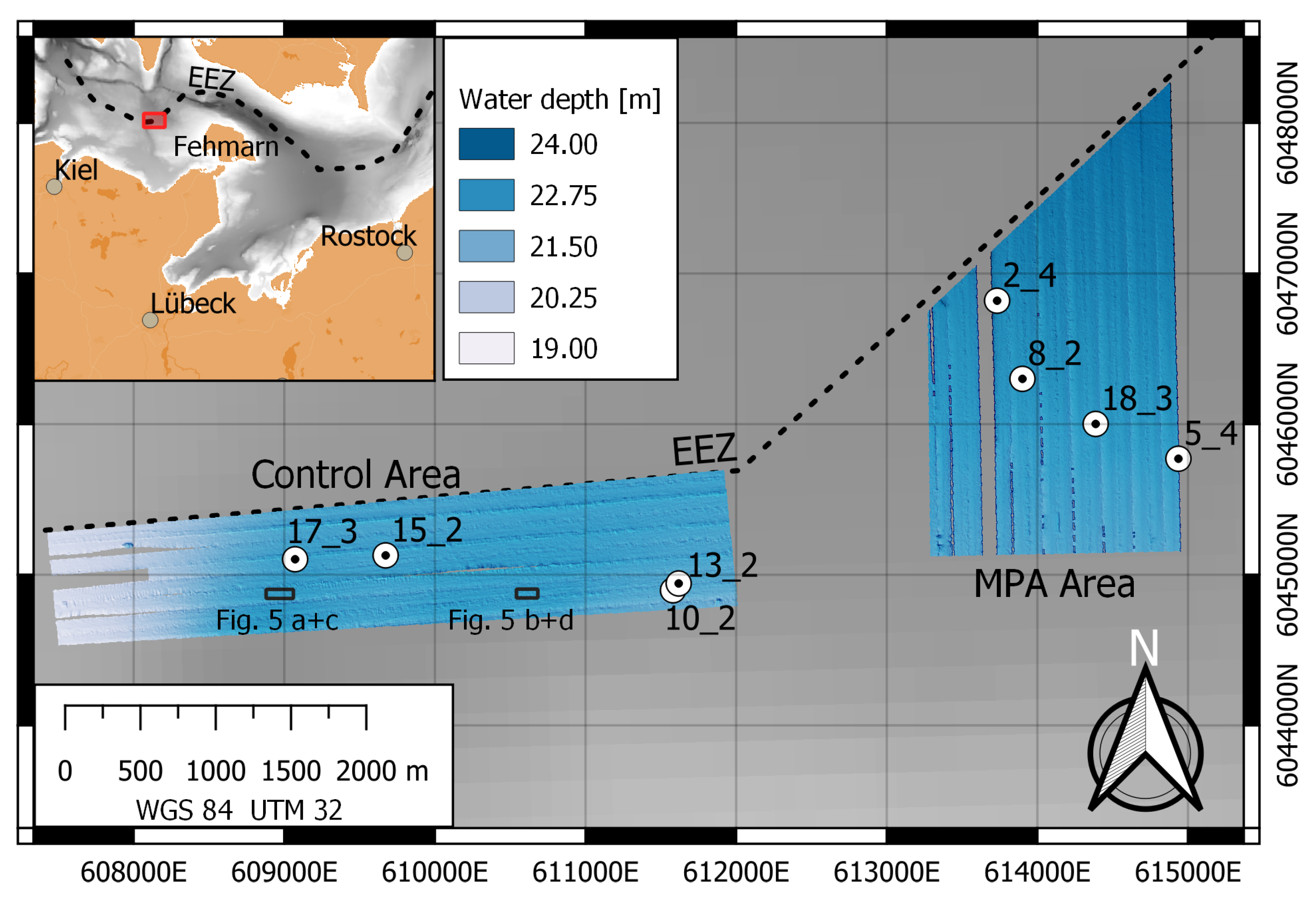
The study site is located 17 km west of the island Fehmarn in the German EEZ of the Baltic Sea and includes 4.7 km2 of the designated Marine Protection Area (MPA) “Fehmarn Belt” [19] and a 3.7 km2 Control area (Control), which are spaced 1.7 km apart. The first survey of the study site was carried out in 2020 on the 28th/29th of May and the second one in 2021 on the 11th of June. An overview of the investigation site is shown in Figure 1. Geologically, to the south-east, the sites adjoin an abrasion platform, which extends west of Fehmarn and is composed of lag-deposits [20]. Lag deposits are composed of coarse sand to gravelly material on underlying till, where the wave action washes out the finer material, leaving the coarse sediment behind [21]. Commonly, abrasion platforms are surrounded by sandy sediment. Due to the prevailing west winds, most of the material that is remobilized offshore Fehmarn is transported alongshore in an eastwards direction. With the main working area located west of the abrasion platform, the reported sediment composition by [22] is predominantly composed of silt and fine sand. A homogeneous sediment composition in the Baltic Sea basins, including our investigation site, is well documented [23]. Typically, the sediment composition consists mainly of silt with high organic content. A high organic content combined with a high proportion of fine sediments is indicative of cohesive sediment properties. From the Baltic Sea basins, it is known that trawl mark traces are preserved over long periods of time [24].
2.2. Multibeam Echosounder
During the survey EMB267 onboard RV Elisabeth Mann Borgese in 2021, the hull-mounted multibeam echosounder system R2Sonic 2024 (R2SONIC, Inc., Austin, TX, USA) was used to record bathymetric data. The user-controllable settings of the MBES are reported in Table 1 and were kept constant throughout the survey. For onboard data acquisition, the software QINSY (version 8) was used. The processing of the MBES data was conducted utilizing the software Qimera (version 2.2.2). The processing of the bathymetric data followed a standard procedure. It included a roll calibration, a sound speed correction, and the computation of the sounding footprints. To perform the sound speed correction, vertical sound velocity profiles of the water column were measured prior to the MBES survey by a Base X sound velocity profiler. The weak spline filter available in Qimera was applied to remove soundings with significant offsets from the local mean water depth. After the processing in Qimera was finished, soundings and ship track data were exported in an ASCII format.
2.3. Side-Scan Sonar
To demonstrate the transition from an abrasion platform to the basin sediments, side-scan sonar data recorded during cruise EMB238 in 2020 are shown. The data were recorded using a Klein 4000 dual-frequency side-scan sonar (100 and 400 kHz), of which the high frequency is shown here. Data were processed using SonarWiz (Chesapeake), applying manual bottom tracking to remove the water column and an empirical gain normalization. The data were exported in a GeoTIFF format with 0.5 m resolution.
2.4. Ground Truthing
Due to unexpected military operations during the research survey prohibiting the use of bottom-contacting gear, the acoustic ground-truthing had to rely on multicorer (MUC) sampling during a prior research cruise of RV Elisabeth Mann Borgese (EMB238) in 2020 at the same site. To achieve an absolute sampling accuracy of about 1 m, an underwater positioning system (USBL) was mounted on the MUC. The sediment cores taken by the MUC have a maximum penetration depth of 50 cm and were sealed directly after recovery and stored in an upright position. In the laboratory, each short core was cut into 1 cm thick slices. From the center of each slice, a sub-sample was taken for grain size analysis. The sub-samples were chemically treated for 4 h with 5% HCl (hydrochloric acid) at 60 °C to remove carbonate content and for 24 h with 15% H2O2 (hydrogen peroxide) at 60 °C to remove organic matter. In between and after chemical treatments, the samples were rinsed with distilled water until pH neutrality. To evaluate the grain size distribution, the particle analyzer Mastersizer 3000, Malvern Panalytical, was used.
2.5. Data Processing
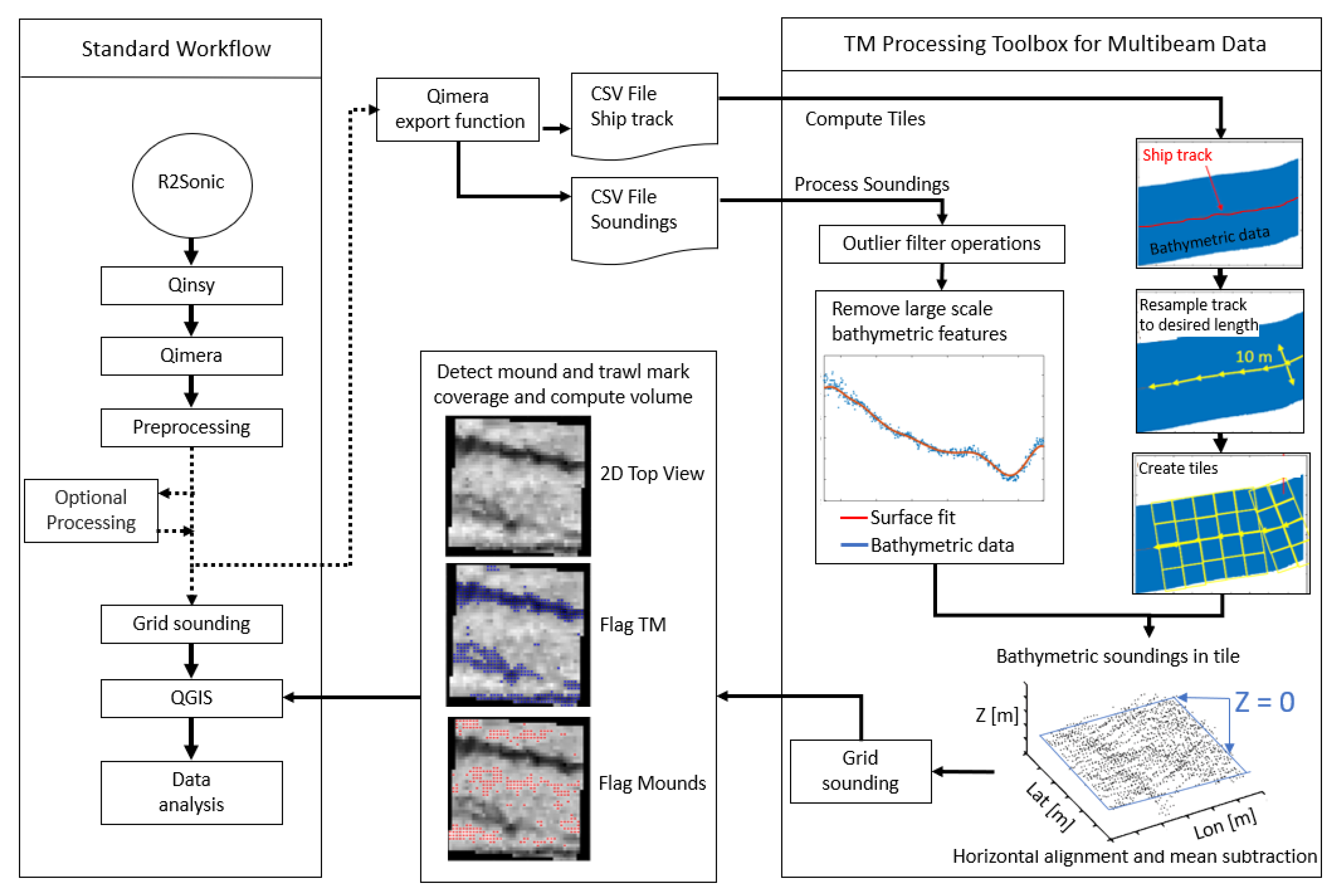
The data processing workflow for trawl mark detection combines a newly developed MATLAB processing tool (The MathWorks, Inc., Natick, MA, USA, version 2018) and QGIS (QGIS version 3.16.1, www.qgis.org) software. An overview of the processing workflow is shown in Figure 2. Accessibility to the code is described in the Supplementary Materials Section. The MATLAB toolbox is integrated as an interface between the data export from Qimera and the data import to QGIS. A major advantage of the workflow design is that the bathymetric data processing within Qimera does not interfere with the import function of the MATLAB toolbox. In this way, the MATLAB toolbox can be used independently of the Qimera processing workflow. The MATLAB toolbox requires ASCII point clouds including Easting, Northing, depth, ping number, and beam number. Shiptrack information is provided by a timestamp (yyyymmddHHMMSS.sss), Easting and Northing.
The following operations are part of the MATLAB processing tool and are described in detail following this overview. Initially, outliers are removed from the data to guarantee stable processing and reliable results. A smoothed surface computed for each ping is subtracted, which effectively removes large-scale bathymetric features. Preprocessing of the data required about 1 day on a standard office computer. Following the export of the ship tracks, 10 m × 10 m tiles were computed along the ship track. The positions of the filtered bathymetric soundings are allocated to the individual tiles. For all soundings located within a tile, a zero-mean surface is calculated, and the soundings are rotated to fit a horizontal surface. For each survey line, a global grid with a constant grid size is created. By allocating the global grid coordinates to each tile, the built-in MATLAB “gridddata” function interpolates the bathymetric soundings to a surface. As a result, each tile is included in the global grid framework and contains a zero-mean bathymetry surface with a constant grid spacing. A threshold is applied to locate all surface points within trawl marks and associated mounds. By summation over the elevation values of all remaining surface points, the volume for trawl marks and mounds was computed. Additionally, the surface area of all valid soundings and the areal coverage percentage of the trawl mark incisions and mound features can be computed. As the final step, the results are exported in the GeoTIFF format for visualization. The GeoTIFF itself consists of multiple bands, containing the bathymetry, the filtered residual bathymetry, the volume and coverage percentage of trawl marks, and the mounds per tile. The average calculation time for a single tile, depending on the CPU, is between 0.02 and 0.06 s.
2.6. Outlier Filtering
The first of five filter stages removes all pings (a ping comprises all data generated by a distinct sound transmission) that contain less than valid soundings of the 1024 available beams. It is assumed these pings are of low quality. The second filter flags all beam angles that contain less than of the maximum number of pings per profile. The maximum amount of pings per profile depends on the length of the individual survey lines. The third filter flags the outer 35 beams on each side. These beams revealed a poor signal-to-noise ratio, which was presumably caused by rapidly changing water column conditions. Following the smoothed surface subtraction, the fourth filter flags values deviating more than ±0.5 m from the zero-mean bathymetry. If tiles overlap by more than (e.g., due to changes in the heading of the research vessel along the survey line), only one tile is kept, and the other is discarded. All flagged soundings are removed before the gridding process.
2.7. Surface Filter Operation
To remove large-scale bathymetric features—such as large current-induced bedforms—from the surface data without affecting small scale features—such as trawl marks— the inbuild MATLAB smooth function was used. The function uses a moving filter to calculate smoothed values for a sliding window with the size of of the 1024 maximum number of soundings per ping. For the moving filter, a robust version of a local regression fit (MathWorks, Inc., version 2018) using a weighted linear least square assigns zero weight to data points outside the six mean absolute deviation (MAD), where
Here, is the value of each depth sounding, and n is the number of soundings. This method removes the large-scale shape of the seafloor without affecting the small-scale morphological features induced by trawling.
2.8. Size of Tiles and Threshold Level
To quantify a morphological trawling impact, trawl marks and mounds must be separated from the natural surface roughness of the corrected bathymetry. To make this distinction for all tiles across the investigation site, the surface values within all tiles must share the same expected value. This is achieved by the zero mean correction of the tiles. However, if the selected tile area is too small, the probability increases that the expected value (0 m for the zero mean corrected tiles) is biased by extreme depth values, which distorts the comparison of different tiles. With increasing tile size, the statistics become more robust at the expense of horizontal resolution, causing a trade-off between quality and resolution. We chose a tile size of 10 × 10 m, containing a maximum of 1600 soundings at a grid resolution of 0.25 m. If there are less than 1600 valid soundings per tile, only the actual number of values is used for the calculations of the results reported in Table 2. After applying the zero mean corrections, the variability of the remaining surface values mainly corresponds to the natural roughness distribution of the seafloor. The average standard deviation along all tiles is 2.2 cm. Anthropogenic features such as trawl marks and mounding have such a significant effect on seafloor roughness that their surface values are located outside of two standard deviations (4.44 cm). However, we set the threshold more conservatively to 5 cm. This threshold was used to automatically mark the trawl mark incisions and mounds, as displayed in Figure 3a,b.
3. Results
An overview of the bathymetric data in the MPA and Control area of Fehmarn Belt is given in Figure 1. Removal of the outer 35 beams reduced the overall coverage, partially causing gaps between the lines. The water depths vary between 19 m and 24 m. The shallowest depths are reached in the eastern part of the Control area, while the deepest area is located in the northern part of the MPA site.
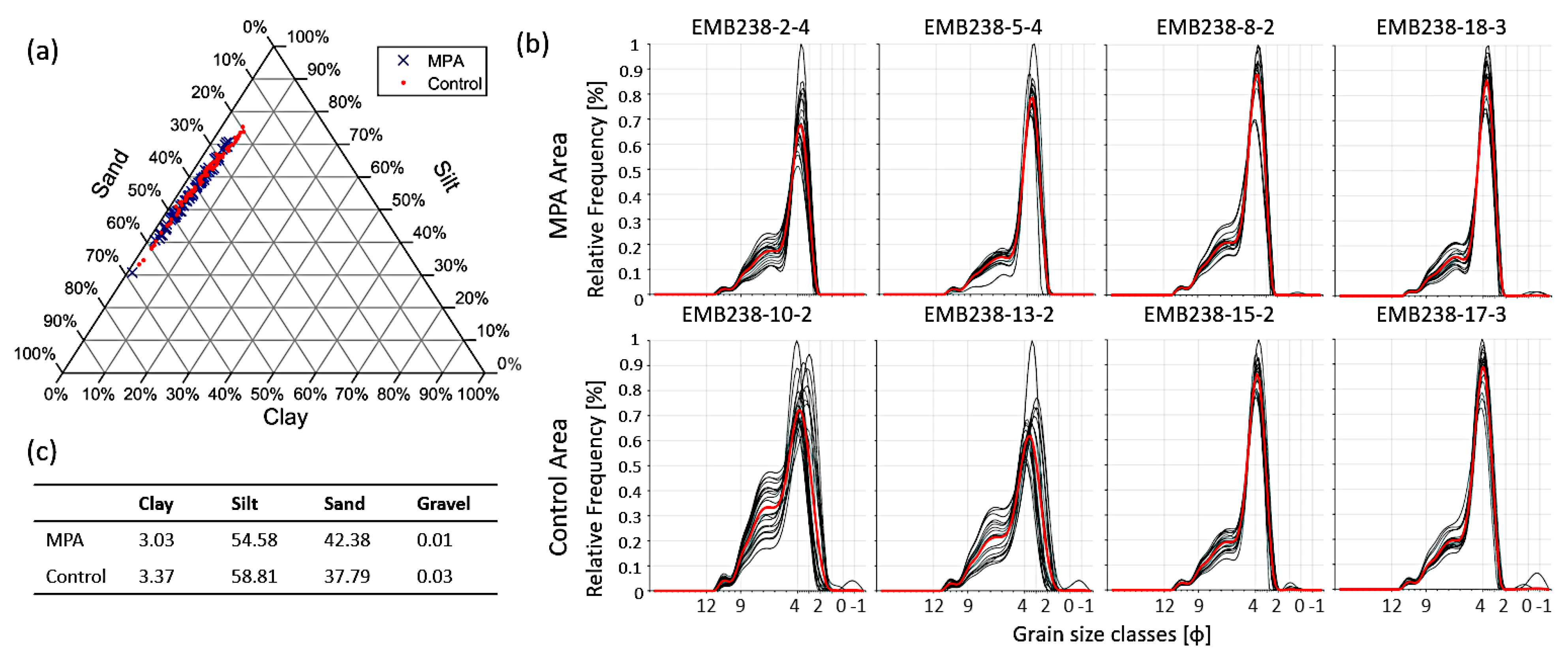
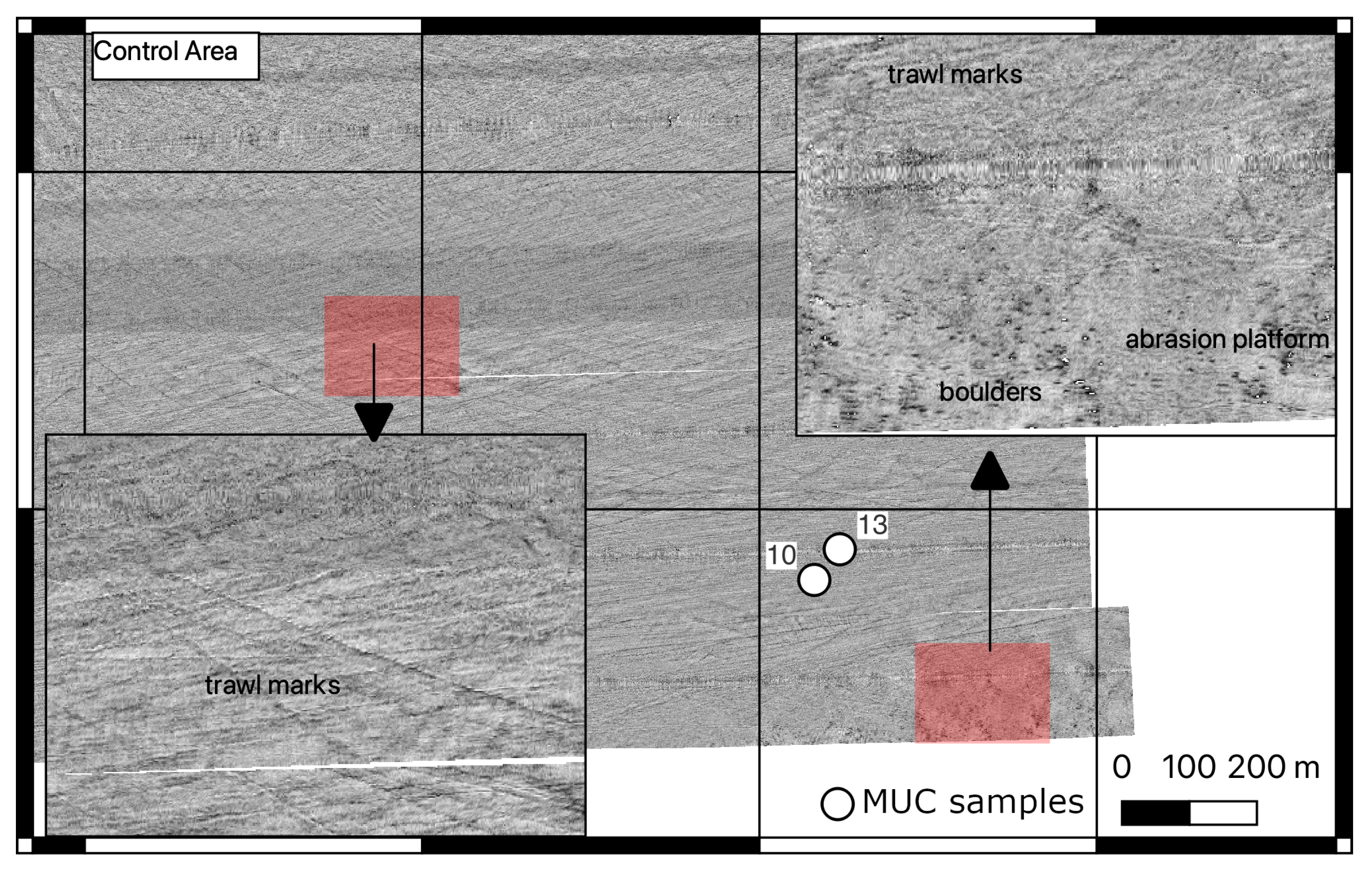
The results of the grain size analysis are similar for the MPA and Control area, with a silt content of 55% and 59% respectively, clay content of 3%, and a sand content of 38% and 42% respectively (Figure 4). Gravel content in the samples is negligible. The increased sand content in the Control area is caused by samples 10-2 and 13-2, which were retrieved close to the abrasion platform west of Fehmarn (Figure 5). The onset of the abrasion platform, including the presence of boulders, is observed in backscatter mosaics (marked in Figure 5). The backscatter images are otherwise dominated by the presence of trawl marks, which are recognizable by alternating backscatter intensities over small scales.
Trawl marks and associated mounds are also observed in the bathymetry grids (example insets shown in Figure 3a,b). Only deeper incisions are accompanied by elevated mounds. In rare cases, mound elevation reaches 30 cm, but most preserved mounds are elevated by 5 cm to 20 cm compared to the surrounding seafloor.
The incision depth of the trawl marks is focused in Figure 3c,d. Their maximum incision depths exceed 25 cm; however, the majority of trawl marks show depths between 10 and 15 cm. Trawl marks can either be continuous features (Figure 3b) or correspond to a series of isolated depressions (Figure 3a). The latter occurs when otter boards are lifted off the seafloor at regular intervals. A further noticeable feature is the merging of different trawl marks, which increase the incision depth (examples can be observed in the south of Figure 3d).
The clear segmentation of trawl marks and mounds following processing allows for an area-wide calculation of morphological parameters (Table 2). Here, a slightly stronger impact of trawling activity is apparent in the Control area, where 5.29% of the seafloor is covered by trawl marks, compared to 3.05% in the MPA site. In total, the volume of trawl mark incisions is 11,357 m3 in the Control and 6620 m3 in the MPA site. Less area is covered by mounds compared to the area covered by trawl marks, with 2.03% in the Control and 0.93% in the MPA site. This is in line with observations at a smaller scale (Figure 3). The total volume of the mounds is 3700 m3 in the Control and 1697 m3 in the MPA site. Therefore, the volume of sediment missing in the trawl marks exceeds the volume of sediment comprising the mounds by factors of 3.1 and 3.9, respectively. Furthermore, the volumetric sediment deficit was calculated from the difference between the sediment volume missing due to the trawl marks and the volume of the mounds (Table 2). The volumetric sediment deficit is 7676 m3 in the Control and 4923 m3 in the MPA site. To normalize the volume in m3 to an area of 1 km2, the sediment deficit is divided by the total area covered by tiles (Table 2). This is equal to 2722 m3 km−2 missing sediment in the Control area and 1709 m3 km−2 missing sediment in the MPA area.
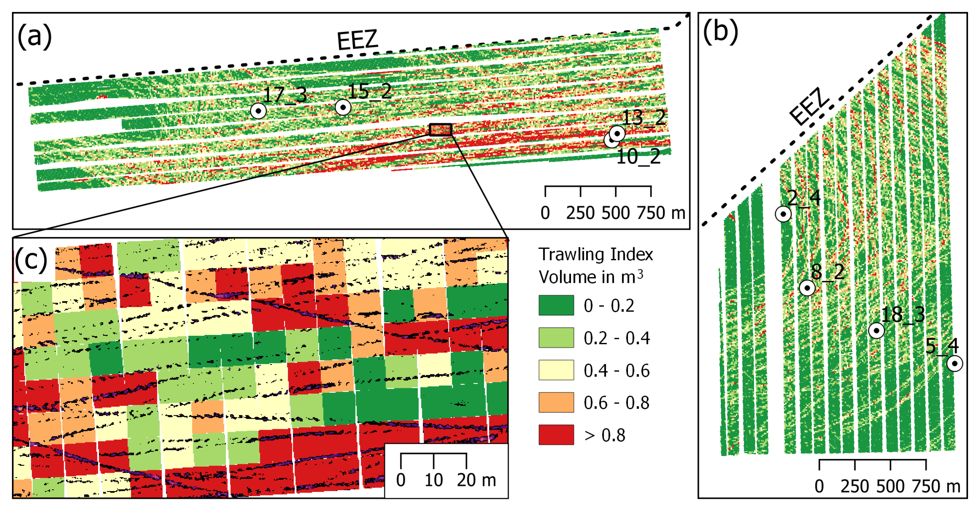
Given that trawl mark incisions are reliably associated with trawl mark activity, while mounds are not always observed (Figure 3), the volume of missing sediment can be utilized as an index of the past trawling intensity. The amount of missing sediment in m per 10 m × 10 m tile is displayed in Figure 6. A classification of the displaced sediment in five classes allows a graphical representation of the impact of trawling on seafloor integrity. It is observed that the strongest impact is located in the southern part of the Control area, directly adjacent to the abrasion platform. Northwards, the morphological impact decreases. At the very south of the Control area, in the region of the abrasion platform where boulders occur, no trawling impact is visible. In the MPA area, the largest physical impact is observed towards the north, while the physical impact decreases towards the south.
4. Discussion
A general limitation when tracking the physical impact of bottom trawling with acoustic methods is the water depth and sediment composition on the seafloor, which needs to be sufficiently cohesive to preserve trawl marks. When quickly remobilized by current or wave action, the physical impact on the seafloor surface (not accounting for disturbance of the sediment column, which may be of ecological importance [25]) is not long-lasting and is not tracked by acoustic methods. With this limitation in mind, recent studies convincingly defined trawl mark density—and thus the indirectly physical impact of bottom trawling—by using the number of trawl marks per km [16,17]. A disadvantage of that approach that made it not applicable in our area is the required digitization of trawl marks to calculate their lengths. Due to the heterogeneous appearance and oftentimes non-continuous nature of the trawl marks, sometimes resembling a series of holes rather than an elongated line (Figure 3), this is a task that is difficult to automate and is time-consuming for human experts. Potentially, this could be achieved by training a neural network similar to recent approaches in boulder mapping [26]. However, the training of a model to recognize trawl marks would be difficult because of the different shapes and scales involved (from holes with few decimeters in diameter to several-kilometer-long lines) [27]. In recent years, new methods based on morphological parameters to classify seafloor features on larger spatial scales were developed [28,29]. Since trawl marks are significant local depressions compared to the surrounding seafloor, parameters such as slope and bathymetric positioning index can be used for their visualization. However, the morphological appearances of trawl marks comprise both linear depressions and isolated holes. Therefore, it is difficult to automatically derive a local trawling intensity from several interacting parameters, as has been suggested for ridges and valley bottoms [28,29,30]. A manual interpretation, on the other hand, is infeasible, especially when considering regular monitoring approaches to map the physical integrity of the seafloor over time. A further disadvantage of using length to identify physical impact is the merging of trawl marks in areas of high impact (Figure 3d). Here, the total impact would be underestimated because the different trawl mark generations cannot be differentiated. Further analysis would be required to assess the impact of such underestimation.
The incision depth of trawl marks in the Fehmarn Belt is in line with other studies conducted in the Baltic Sea [31] or in comparable settings (e.g., [32]). The calculation of sediment displacement in small (10 m × 10 m) tiles as conducted in this study does not require knowledge of individual trawl marks and thus can be rapidly applied over larger areas of interest. The volumetric difference between trawl marks and associated mounds agrees with a 30% increased net sediment transport between Baltic Sea basins induced by bottom trawling, which was recently postulated by Porz et al. [33] based on a combination of models and fieldwork. Assuming a porosity of 60% for near-surface deposits, a density of 2.65 g cm and using the difference between incision and mound values (Table 2), a maximum of 5218 tons of sediment were resuspended from the original trawling sites in the MPA area (1812 tons per km) and 8137 tons of sediment in the Control area (2721 tons per km). These values are likely underestimated due to the applied threshold value, and the underestimation of narrow trawl mark incision depths during the gridding of the MBES point cloud. A disadvantage of the method is the potential impact of morphological features such as ripple fields or pockmarks on the volume calculation. At the current state, the method cannot be applied in areas where such features occur in the Baltic Sea. However, ripples and dunes typically occur rather close to the coastline and not in the Baltic Sea basins, which show a smooth morphology [23,34,35]. Additionally, areas with pronounced morphological features (e.g., the boulders in the south of Figure 5) cause damage to bottom-touching gear and are thus generally avoided by fishing vessels.
Figure 6 represents the cumulative physical impact of trawling over several years. Trawl marks in cohesive sediment below the wave base and in areas of low sedimentation rates may be preserved for several years [32]. Therefore, the sediment displacement within the trawl marks can be thought of as a long-term impact that—in the Baltic Sea basins—will disappear only over longer time periods. To capture the restoration of physical impacts over shorter periods of time, the mounds piled up by the otter boards may be more promising. The mounds are remobilized faster, as is apparent by the fact that not all trawl marks are accompanied by mounds (Figure 3a,b). Therefore, the volume of mounds could be used as an indicator for recent bottom fishing activity or regeneration of natural seafloor conditions in newly established fishery-exclusion areas. Conceivably, the method is also applicable to quantify the impact of anchor scours, as recently surveyed by [36].
5. Conclusions
An index measuring the physical impact of bottom trawling on the seafloor was developed based on high-resolution bathymetric data, measuring the sediment displaced during trawling in 10 m × 10 m cells. The index is applicable to the Baltic Sea basins (and comparable regions) with cohesive seafloor sediments and absent morphological features of natural origin. Because the index is calculated with minor involvement of human expert knowledge, it can be used for monitoring purposes. Future work will include studies on the impact of survey settings and instrument type and the impact of different fishing gear on seafloor integrity.
Supplementary Materials
The following datafiles can be downloaded at https://www.mdpi.com/article/10.3390/rs14122782/s1, Figure S1 shows the MBES trackline planning during the EMB267 survey. To get access to the GitHub repository containing the MATLAB code of the MBES Processing Toolbox, please use the following link: https://github.com/SchoenkeM/MBES_Processing_Toolbox/releases/latest. Version 1.0.0 was used in this publication.
Author Contributions
Conceptualization, P.F. and M.S.; methodology, M.S. and P.F.; software, M.S.; formal analysis, M.S.; investigation, M.S., P.F. and D.C.; resources, P.F.; data curation, M.S. and P.F.; writing—original draft preparation, M.S. and P.F.; writing—review and editing, D.C.; visualization, M.S.; project administration, P.F.; funding acquisition, P.F. All authors have read and agreed to the published version of the manuscript.
Funding
This research was funded by the Bundesministerium für Bildung und Forschung (BMBF), project ”DAM pilot mission: Exclusion of mobile bottom-contact fishing in marine protected areas of the German EEZ of the North Sea and Baltic Sea”, grant number 03F0848A.
Data Availability Statement
The MBES raw data presented in this study are stored on dedicated servers at the Leibniz Institute for Baltic Sea Research Warnemünde and are available from the corresponding author at reasonable request. The point cloud data (ship logs and soundings) used for the calculations are available under https://doi.org/10.5281/zenodo.6597161 (last accessed: 7 June 2022).
Acknowledgments
We gratefully thank the master and crew of RV Elisabeth Mann Borgese for their support during our research cruises EMB238 and EMB267. We would like to thank the other scientists on those cruises for their tremendous support, who always found time to assist us despite the lack of staff and time due to Coronavirus restrictions. We gratefully thank our technician Frank Pohl for their extraordinary support during the fieldwork. Further, we would like to thank our intern Emmi Schleweis who did an excellent job with the particle size analysis in the lab. The constructive comments of two reviewers improved the manuscript.
Conflicts of Interest
The authors declare no conflict of interest.
References
- Micallef, A.; Krastel, S.; Savini, A. (Eds.) Submarine Geomorphology; Springer International Publishing: Springer International Publishing, 2018; Volume 2018, pp. 503–552. [Google Scholar] [CrossRef]
- Grip, K.; Blomqvist, S. Marine nature conservation and conflicts with fisheries. AMBIO 2020, 49, 1328–1340. [Google Scholar] [CrossRef] [PubMed] [Green Version]
- Amoroso, R.O.; Pitcher, C.R.; Rijnsdorp, A.D.; McConnaughey, R.A.; Parma, A.M.; Suuronen, P.; Eigaard, O.R.; Bastardie, F.; Hintzen, N.T.; Althaus, F.; et al. Bottom trawl fishing footprints on the world’s continental shelves. Proc. Natl. Acad. Sci. USA 2018, 115, E10275–E10282. [Google Scholar] [CrossRef] [PubMed] [Green Version]
- Oberle, F.K.; Storlazzi, C.D.; Hanebuth, T.J. What a drag: Quantifying the global impact of chronic bottom trawling on continental shelf sediment. J. Mar. Syst. 2016, 159, 109–119. [Google Scholar] [CrossRef]
- Bradshaw, C.; Tjensvoll, I.; Sköld, M.; Allan, I.J.; Molvaer, J.; Magnusson, J.; Naes, K.; Nilsson, H.C. Bottom trawling resuspends sediment and releases bioavailable contaminants in a polluted fjord. Environ. Pollut. 2012, 170, 232–241. [Google Scholar] [CrossRef]
- Mazor, T.; Pitcher, C.R.; Rochester, W.; Kaiser, M.J.; Hiddink, J.G.; Jennings, S.; Amoroso, R.; McConnaughey, R.A.; Rijnsdorp, A.D.; Parma, A.M.; et al. Trawl fishing impacts on the status of seabed fauna in diverse regions of the globe. Fish Fish. 2021, 2021. 22, 72–86. [Google Scholar] [CrossRef]
- Palanques, A.; Puig, P.; Guillén, J.; Demestre, M.; Martín, J. Effects of bottom trawling on the Ebro continental shelf sedimentary system (NW Mediterranean). Cont. Shelf Res. 2014, 72, 83–98. [Google Scholar] [CrossRef]
- Pope, J.G. Input and Output Controls: The Practice of Fishing Effort and Catch Management in Responsible Fisheries. In A Fishery Manager’s Guidebook, 2nd ed.; John Wiley & Sons, Inc.: Hoboken, NJ, USA, 2009; pp. 220–252. [Google Scholar] [CrossRef]
- European Commission. Roadmap for Maritime Spatial Planning: Achieving Common Principles in the EU. COM (2008) 791 final. Off. J. Eur. Union 2008, 2008, 12. [Google Scholar]
- Benn, A.R.; Weaver, P.P.; Billet, D.S.; van den Hove, S.; Murdock, A.P.; Doneghan, G.B.; le Bas, T. Human activities on the deep seafloor in the North East Atlantic: An assessment of spatial extent. PLoS ONE 2010, 5, e12730. [Google Scholar] [CrossRef] [Green Version]
- Smith, C.J.; Banks, A.C.; Papadopoulou, K.N. Improving the quantitative estimation of trawling impacts from sidescan-sonar and underwater-video imagery. ICES J. Mar. Sci. 2007, 64, 1692–1701. [Google Scholar] [CrossRef] [Green Version]
- Russo, T.; D’Andrea, L.; Parisi, A.; Cataudella, S. VMSbase: An R-Package for VMS and logbook data management and analysis in fisheries ecology. PLoS ONE 2014, 9, e100195. [Google Scholar] [CrossRef]
- Mérillet, L.; Kopp, D.; Robert, M.; Salaün, M.; Méhault, S.; Bourillet, J.F.; Mouchet, M. Are trawl marks a good indicator of trawling pressure in muddy sand fishing grounds? Ecol. Indic. 2018, 85, 570–574. [Google Scholar] [CrossRef] [Green Version]
- Piet, G.J.; Hintzen, N.T. Indicators of fishing pressure and seafloor integrity. ICES J. Mar. Sci. 2012, 69, 1850–1858. [Google Scholar] [CrossRef]
- Hansen, R.E. Mapping the ocean floor in extreme resolution using interferometric synthetic aperture sonar. Proc. Meet. Acoust. 2019, 38, 10. [Google Scholar] [CrossRef] [Green Version]
- Bruns, I.; Holler, P.; Capperucci, R.M.; Papenmeier, S.; Bartholomä, A. Identifying trawl marks in north sea sediments. Geosciences 2020, 10, 422. [Google Scholar] [CrossRef]
- Gournia, C.; Fakiris, E.; Papatheodorou, G.; Geraga, M.; Williams, D.P. Automatic detection of trawl-marks in sidescan sonar images through spatial domain filtering, employing haar-like features and morphological operations. Geosciences 2019, 9, 214. [Google Scholar] [CrossRef] [Green Version]
- Hinz, H.; Prieto, V.; Kaiser, M.J. Trawl disturbance on benthic communities: Chronic effects and experimental predictions. Ecol. Appl. 2009, 19, 761–773. [Google Scholar] [CrossRef]
- Bundesamt für Naturschutz. Managementplan für das Naturschtzgebiet “Fehmarnbelt” (MPFmb). In Bundesanzeiger; 8 February 2022; BAnz AT 08.02.2022 B6; pp. 1–132. [Google Scholar]
- Feldens, P.; Diesing, M.; Schwarzer, K.; Heinrich, C.; Schlenz, B. Occurrence of flow parallel and flow transverse bedforms in Fehmarn Belt (SW Baltic Sea) related to the local palaeomorphology. Geomorphology 2015, 231, 53–62. [Google Scholar] [CrossRef]
- Tauber, F.; Lemke, W. Map of sediment distribution in the western Baltic Sea (1: 100,000), Sheet “Darß”. Dtsch. Hydrogr. Z. 1995, 47, 171–178. [Google Scholar] [CrossRef]
- BSH. Anleitung zur Kartierung des Meeresbodens Mittels Hochauflösender Sonare in den Deutschen Meeresgebieten; Report; Bundesamt für Seeschifffahrt und Hydrographie (BSH): Hamburg and Rostock, Germany, 2016. [Google Scholar]
- Tauber, F. Meeresbodensedimente in der Deutschen Ostsee: Fehmarn, Karte Nr. 2932. Maßstab 1:100 000; Map; Bundesamt für Seeschifffahrt und Hydrographie (BSH): Hamburg and Rostock, Germany, 2012; ISBN 978-3-86987-381-7. [Google Scholar]
- Bunke, D.; Leipe, T.; Moros, M.; Morys, C.; Tauber, F.; Virtasalo, J.J.; Forster, S.; Arz, H.W. Natural and Anthropogenic Sediment Mixing Processes in the South-Western Baltic Sea. Front. Mar. Sci. 2019, 6, 677. [Google Scholar] [CrossRef]
- Kaiser, M.J.; Collie, J.S.; Hall, S.J.; Jennings, S.; Poiner, I.R. Modification of marine habitats by trawling activities: Prognosis and solutions. Fish Fish. 2002, 3, 114–136. [Google Scholar] [CrossRef]
- Feldens, P.; Westfeld, P.; Valerius, J.; Feldens, A.; Papenmeier, S. Automatic detection of boulders by neural networks. A comparison of multibeam echo sounder and side-scan sonar performance. Hydrogr. Nachrichten 2021, 119, 6–17. [Google Scholar]
- Cai, Z.; Fan, Q.; Feris, R.S.; Vasconcelos, N. A Unified Multi-scale Deep Convolutional Neural Network for Fast Object Detection. In ECCV 2016: Computer Vision—ECCV 2016; Springer: Cham, Switzerland, 2016; Volume 9908, pp. 354–370. [Google Scholar] [CrossRef] [Green Version]
- Pendleton, E.A.; Sweeney, E.M.; Brothers, L.L. Optimizing an Inner-Continental Shelf Geologic Framework Investigation through Data Repurposing and Machine Learning. Geosciences 2019, 9, 231. [Google Scholar] [CrossRef] [Green Version]
- de Oliveira, N.; Bastos, A.C.; da Silva Quaresma, V.; Vieira, F.V. The use of Benthic Terrain Modeler (BTM) in the characterization of continental shelf habitats. Geo-Mar. Lett. 2020, 40, 1087–1097. [Google Scholar] [CrossRef]
- Janowski, L.; Wroblewski, R.; Rucinska, M.; Kubowicz-Grajewska, A.; Tysiac, P. Automatic classification and mapping of the seabed using airborne LiDAR bathymetry. Eng. Geol. 2022, 301, 106615. [Google Scholar] [CrossRef]
- Hoffmann, J.J.; Schneider von Deimling, J.; Schröder, J.F.; Schmidt, M.; Held, P.; Crutchley, G.J.; Scholten, J.; Gorman, A.R. Complex Eyed Pockmarks and Submarine Groundwater Discharge Revealed by Acoustic Data and Sediment Cores in Eckernförde Bay, SW Baltic Sea. Geochem. Geophys. Geosyst. 2020, 21, e2019GC008825. [Google Scholar] [CrossRef]
- Bradshaw, C.; Jakobsson, M.; Brüchert, V.; Bonaglia, S.; Mörth, C.M.; Muchowski, J.; Stranne, C.; Sköld, M. Physical Disturbance by Bottom Trawling Suspends Particulate Matter and Alters Biogeochemical Processes on and Near the Seafloor. Front. Mar. Sci. 2021, 8, 683331. [Google Scholar] [CrossRef]
- Porz, L.; Zhang, W.; Schrum, C. Natural and anthropogenic influences on the development of mud depocenters in the southwestern Baltic Sea. Oceanologia, 2022; in press. [Google Scholar] [CrossRef]
- Feldens, P.; Schwarzer, K.; Hübscher, C.; Diesing, M. Genesis and Sediment Dynamics of a Subaqueous Dune Field in Fehmarn Belt (South-Western Baltic Sea). In Ergebnisse aktueller Küstenforschung: Beiträge der 26. Jahrestagung des Arbeitskreises "Geographie der Meere und Küsten", 25–27 April 2008 in Marburg (Marburger Geographische Schriften); Marburger Geographische Schriften: Marburg, Germany, 2009; pp. 80–97. [Google Scholar]
- Beisiegel, K.; Tauber, F.; Gogina, M.; Zettler, M.L.; Darr, A. The potential exceptional role of a small Baltic boulder reef as a solitary habitat in a sea of mud. Aquat. Conserv. Mar. Freshw. Ecosyst. 2019, 29, 321–328. [Google Scholar] [CrossRef]
- Watson, S.J.; Ribó, M.; Seabrook, S.; Strachan, L.J.; Hale, R.; Lamarche, G. The footprint of ship anchoring on the seafloor. Sci. Rep. 2022, 12, 7500. [Google Scholar] [CrossRef]
Figure 1.
Overview of the investigation sites MPA and Control in the southern Baltic Sea. The location of short sediment cores used for sedimentological ground-truthing is shown by white circles. The associated labels show the station number during cruise EMB238.
Figure 1.
Overview of the investigation sites MPA and Control in the southern Baltic Sea. The location of short sediment cores used for sedimentological ground-truthing is shown by white circles. The associated labels show the station number during cruise EMB238.

Figure 2.
Overview of the processing workflow. The soundings and ship track data were exported from Qimera in ASCII format to serve as the input data set for the MBES processing tool. In both cases, the x,y-components of the data correspond to UTM coordinates in meters (UTM 32N WGS84), while the z-component represents the measured water depth in meters. Ping and beam numbers were used for filtering purposes. For the output, the soundings were rasterized in the GeoTIFF format with a grid resolution of 0.25 m.

Figure 3.
(a,b) show the elevation of the seafloor relative to the zero-mean surface with depressions in red and mounds in blue colors. Data are based on the 2021 multibeam survey. (c,d) show the same regions, respectively, but focus on the depressions, which are almost exclusively trawl marks. In the south of (d), the merging of several trawl marks into one can be observed. Refer to Figure 1 for locations.

Figure 4.
Summary of the grain size analysis. The sample locations are shown in Figure 1. (a) The ternary sand–silt–clay plot demonstrates low clay contents and the sedimentological similarity between the MPA and Control site. (b) Grain size distributions of the individual samples. Each sample was measured 12 times, with the red curve showing the average results. The table (c) shows the average of sediment data categorized by grain size class and split between MPA and Control site.

Figure 5.
Side-scan sonar backscatter map in the south-eastern part of the Control area. Backscatter values are homogeneous throughout the Control and MPA area, and backscatter features are dominated by trawl marks only recognizable at small scales. Notable is the abrasion platform in the south, where boulders are present on the seafloor and trawl marks disappear.

Figure 6.
Visualization of the proposed displaced sediment trawling index based on the volume of the trawl mark incisions per 10 m × 10 m tile. High values, displayed in red colors, indicate a high physical impact. Shown are (a) the Control area, (b) the MPA area and (c) a zoomed-in view with the trawl mark incision depths (compare with Figure 3c,d). The locations of sediment cores are indicated by white circles. The analysis is based on the 2021 multibeam echo sounder survey.


Table 1.
Multibeam echosounder parameters during data acquisition.
| Parameter | EMB267, Survey 2021 |
|---|---|
| Fan angle [°] | 140 |
| Frequency [kHz] | 400 |
| Puls length [μs] | 15 |
| Source level [dB] | 194 |
| Gain [dB] | 7 |
| Spreading [ ] | 40 |
| Absorption [ ] | 110 |
| Soundings per ping | 1024 |
| Snippet data | yes |
| Multi-frequency data | no |
| Absolute dB values | no |
| Avg. survey speed [kn] | 4.5–5 |
Table 2.
Morphological parameters of the identified trawl marks and mounds; values are rounded to two decimal digits.
Table 2.
Morphological parameters of the identified trawl marks and mounds; values are rounded to two decimal digits.
| Parameter | MPA Area | Control Area |
|---|---|---|
| Number of tiles | 29,160 | 29,069 |
| Tile’s coverage [km] | 2.88 | 2.82 |
| Area covered by trawl marks [%] | 3.05 | 5.29 |
| Area covered by trawl marks [km] | 0.09 | 0.15 |
| Volume of trawl marks [m] | 6620 | 11,375 |
| Area covered by mounds [%] | 0.93 | 2.03 |
| Area covered by mounds [km] | 0.01 | 0.04 |
| Volume of mounds [m] | 1697 | 3700 |
Publisher’s Note: MDPI stays neutral with regard to jurisdictional claims in published maps and institutional affiliations. |
© 2022 by the authors. Licensee MDPI, Basel, Switzerland. This article is an open access article distributed under the terms and conditions of the Creative Commons Attribution (CC BY) license (https://creativecommons.org/licenses/by/4.0/).
Share and Cite
MDPI and ACS Style
Schönke, M.; Clemens, D.; Feldens, P. Quantifying the Physical Impact of Bottom Trawling Based on High-Resolution Bathymetric Data. Remote Sens. 2022, 14, 2782. https://doi.org/10.3390/rs14122782
AMA Style
Schönke M, Clemens D, Feldens P. Quantifying the Physical Impact of Bottom Trawling Based on High-Resolution Bathymetric Data. Remote Sensing. 2022; 14(12):2782. https://doi.org/10.3390/rs14122782
Chicago/Turabian StyleSchönke, Mischa, David Clemens, and Peter Feldens. 2022. "Quantifying the Physical Impact of Bottom Trawling Based on High-Resolution Bathymetric Data" Remote Sensing 14, no. 12: 2782. https://doi.org/10.3390/rs14122782
Note that from the first issue of 2016, this journal uses article numbers instead of page numbers. See further details here.