
GNSS-IR Measurements of Inter Annual Sea Level Variations in Thule, Greenland from 2008–2019
by
 , , , and
Trine S. Dahl-Jensen
1,* ,
,
Ole B. Andersen
1,
Simon D. P. Williams
2,
Veit Helm
3 and
Shfaqat A. Khan
1 1
Danish National Space Centre, Technical University of Denmark, 2800 Lyngby, Denmark
2
National Oceanography Center, Liverpool L3 5DA, UK
3
Alfred Wegener Institute, Helmholtz Centre for Polar and Marine Research, 27570 Bremerhaven, Germany
*
Author to whom correspondence should be addressed.
Remote Sens. 2021, 13(24), 5077; https://doi.org/10.3390/rs13245077
Submission received: 5 November 2021
/
Revised: 8 December 2021
/
Accepted: 9 December 2021
/
Published: 14 December 2021
(This article belongs to the Section Ocean Remote Sensing)
Abstract
:Studies of global sea level often exclude Tide Gauges (TGs) in glaciated regions due to vertical land movement. Recent studies show that geodetic GNSS stations can be used to estimate sea level by taking advantage of the reflections from the ocean surface using GNSS Interferometric Reflectometry (GNSS-IR). This method has the immediate benefit that one can directly correct for bedrock movements as measured by the GNSS station. Here we test whether GNSS-IR can be used for measurements of inter annual sea level variations in Thule, Greenland, which is affected by sea ice and icebergs during much of the year. We do this by comparing annual average sea level variations using the two methods from 2008–2019. Comparing the individual sea level measurements over short timescales we find a root mean square deviation (RMSD) of 13 cm, which is similar to other studies using spectral methods. The RMSD for the annual average sea level variations between TG and GNSS-IR is large (18 mm) compared to the estimated uncertainties concerning the measurements. We expect that this is in part due to the TG not being datum controlled. We find sea level trends from GNSS-IR and TG of −4 and −7 mm/year, respectively. The negative trend can be partly explained by a gravimetric decrease in sea level as a result of ice mass changes. We model the gravimetric sea level from 2008–2017 and find a trend of −3 mm/year.
1. Introduction
Global sea level is currently rising at a rate of 3 mm/year as a result of ongoing climate change [1,2]. The distribution of local sea level rise is not uniform and thus some areas experience significantly higher than average sea level rise while other areas experience decreasing sea level [2,3].
Local relative sea level change is traditionally measured using Tide Gauges (TGs) while global sea level studies are often based on a combination with satellite altimetry. In general there are not many TGs in the arctic regions, which reduces the possibility of studying the local sea level change. Furthermore, in order to use TGs for studies of global eustatic sea level change, the TG measurements need to be corrected for bedrock movements of the solid earth. In glaciated regions, such as Greenland, the bedrock movement is large and complicated to model and is a combination of elastic movement caused by ongoing ice mass variability and a viscoelastic component caused by past ice variability over thousands of years (also known as the glacial isostatic adjustment). There is a large uncertainty on the modeled uplift, and therefore TG data from these areas are typically omitted from studies of global eustatic sea level [1,4].
Recent studies show that, under the right conditions, relative sea level change can be measured using GNSS Interferometric Reflectometry (GNSS-IR) [5,6]. Usage of GNSS stations to measure sea level has the immediate benefit that the bedrock movement is simultaneously measured with a high precision at the site allowing the local eustatic sea level to be calculated directly. The uncertainty on individual measurements of sea level is considerably higher using GNSS-IR compared to TGs. However, averages taken over a day are almost directly comparable and correlate very well [6]. A higher accuracy on the individual measurements can potentially be found using inverse modelling methods when necessary [7].
Larson et al. [6] studied sea level variations using GNSS-IR from a GNSS station installed at Friday Harbour, Washington. Though the GNSS station was installed with the purpose of studying tectonic movement, they found good agreement with a nearby TG for monthly averages over a 10 year period. The area is in some ways ideal for reflectometry studies as it experiences little vertical land movement and is not affected by sea ice. Kim and Park [8] use GNSS-IR to study sea level in St. Michael, Alaska using a GNSS station installed in 2018 and compare with nearby TGs. The results are promising, however, the closest TG with actual sea level data is in Unalakleet, 74 km from St. Michael.
In this study we will test whether GNSS-IR can be used for measurements of inter annual sea level variations in a complicated glaciated region affected by large vertical land movement, sea ice and icebergs.
In Greenland, an extensive network of 58 permanent geodetic GNSS stations, called GNET, have been installed on bedrock between 2007 and 2009 [9,10]. The main purpose of GNET is to investigate changes in the Greenland ice sheet by continuously measuring bedrock uplift. Tabibi et al. [11] used four GNET stations as well as four Antarctic stations to study tidal constituents in Arctic regions from GNSS-IR. Unfortunately the four used GNET stations (KULL, QAAR, PLPK and KULU) are not co-located with a TG for direct comparison.
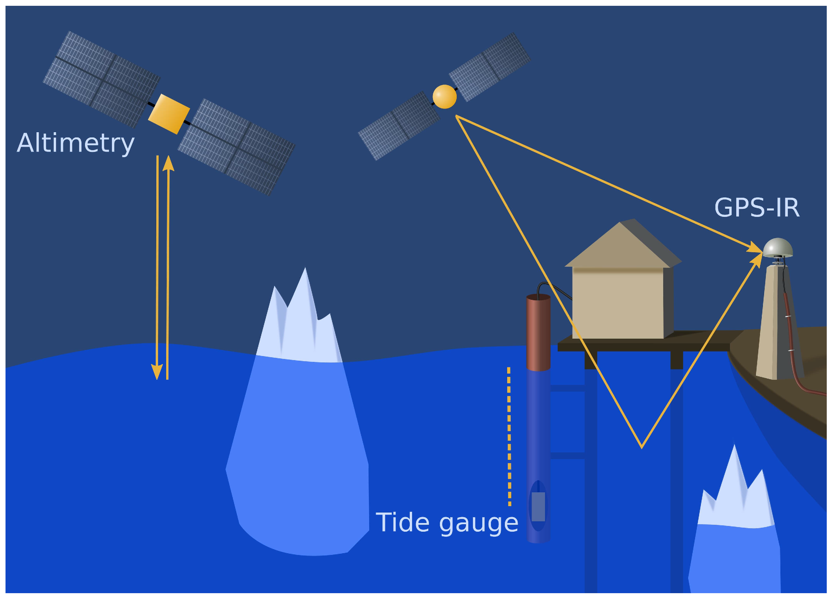
Here, we compare sea level variations measured by GNSS-IR from a GNET GNSS station located at Thule Airbase with results from a nearby TG station together with satellite altimetry data. The three methods are illustrated in Figure 1. GNSS-IR and TG both measure the local sea level variations while altimetry measures the absolute sea level. In order to compare the GNSS-IR and TG measurements with altimetry we will have to correct for vertical bedrock movement, as measured by the GNSS station.
2. Materials and Methods
2.1. Sea Level Measurements
The TG in Thule is maintained by DTU Space and measures sea level every 5 min. It is not datum controlled, thus, there may be gross errors that are unidentified in the data set. It was installed in 2006, however, the data from the TG was of poor quality until late 2007 when it was maintained and moved to a new location. Therefore, only data from 2008 and onwards are used in this study. The station was returned to the original position in September 2015 (Figure 2c). We include the data after this date in this study as the data quality is similar to the 2008–2015 period and otherwise the usable time period will be short.
The GNSS station in Thule is located approximately 60 m from the coast in a bay close to the harbor (Figure 2). The distance between the TG and the GNSS station is less than 2 km from 2008–2015 and shorter after the move. From GNSS-IR we have sub daily estimates of sea surface height from 2002 to early 2020. However, only data from the period covered by the TG is used in this study.
We used the same methodology to measure sea level using GNSS Signal to Noise Ratio (SNR) measurements as described in Larson et al. [6] and Williams et al. [12]. Individual satellite passes are split into ascending and descending nodes and masked using a pre-selected elevation and azimuth mask to select satellite passes where the main reflector should be the water surface. The measured SNR data are translated to a linear scale from decibels-hertz and a low-order polynomial is used to remove the direct signal effect. Spectral analysis of the residual SNR as a function of the wavelength of the carrier signal and the elevation angle of the satellite should produce a peak at a frequency that is related to the height of the antenna above the horizontal reflecting surface, the primary observation in GNSS-IR water level studies. We include corrections for non-stationary reflector height (the effect) [13] and tropospheric delay [14]. We use an initial elevation mask of between 2 and 20 and an azimuth range of between 160 and 290. During the initial Quality Control (QC) process passes with an average azimuth lower than 170, higher than 270 or an estimated reflector height lower than 17 m were removed. The final, iterative, QC process is described in Williams et al. [12]. Maps illustrating the reflection zones (fresnel zones) are included in the supplementary material.
The altimetry data used in this study are the ESA CCI DTU/TUM sea level anomaly [15]. It is based on data from ERS-1, ERS-2, Envisat and Cryosat-2. The data used here is from the period covered by Envisat and Cryosat-2 and an average is calculated over the area between 68.5 and 72 degrees west and 76 and 77 north (Figure 2d).
Both TG and GNSS-IR observations were analyzed using the response method extended with the orthotide formalism [16] in order to remove the tidal signal. The advantage of using this method is as follows: by assuming a smooth admittance function described by a relatively low number of parameters within each tidal band (orthotide parameters) a solution for any constituent can be inferred and hence corrected for. For 2016, removing the ocean tides reduces the RMS of the observed sea level from the TG from 72 cm to 15 cm.
After removing the tides, all sea level data are filtered in order to enhance the inter annual signal. The annual and semi-annual signal is removed using a least squares fit of the two harmonics [17]. By removing the annual and semi-annual signal, the influence of potential gaps in the data on annual average sea level will be smaller. The error in the annual average sea levels from GNSS-IR and TG as well as the annual measured uplift are estimated by calculating the standard deviation of the daily measurement over all periods of 60 daily values. After that the average value of this standard deviation for each year is calculated and from that the standard deviation of the mean is calculated using the number of daily measurements from that year.
The uncertainty of the annual altimetry results are estimated as the standard deviation of the mean from the monthly sea levels after filtering out the annual and bi-annual signal.
In order to be able to compare GNSS-IR and TG results with the altimetry, we need to correct for vertical land movement. For this we use daily positions of the same GNSS station [9,10]. The GNSS station in Thule covers a period from 1999 to present and daily positions are available throughout 2019 with minor gaps.
In order to avoid differences in the annual averages of the TG and GNSS-IR sea level measurements due to gaps in the data series, only data from days where there is data from both methods are used to calculate the annual values.
2.2. Sea Level Change Due to Reduced Gravity
As ice mass is lost in e.g., Greenland and Antarctica, the local gravity attraction drops, resulting in decreasing sea levels. To estimate this gravitational effect, we convolve ice mass change with the Green’s functions for geoid anomaly derived by Wang et al. [18] for elastic Earth model iasp91 with refined crustal structure from Crust 2.0. We use ice mass changes from both Greenland, Antarctica and other glaciers as these may all influence sea levels in Thule.
For the ice mass changes in Antarctica we use the gridded mass balance product from Groh and Horwath [19] which is available until mid 2016. The annual mean sea level change due to reduced gravitational effect from Antarctica is 0.05 mm which is at least an order of magnitude smaller than for Greenland or other glaciers due to the long distance from Thule. The uncertainty on the gravitational results in 2016-2018 is altered to account for this added uncertainty.
For Greenland we interpolate a 2 × 2 km grid of annual ice height changes from 2007–2015 and a 2.5 × 2.5 km grid from 2016–2017 using altimeter data from NASA’s ATM flights [20] supplemented with high resolution ICESat laser altimetry data from 2003 to 2009 [21] and Cryosat-2 data (2011–2017) [22], complemented with ENVISAT data from 2009 to 2012 [23]. The method used to create the height change grid is described in detail by Khan et al. [23].
Mass changes from other glaciers are extracted from an update of the model by Marzeion et al. [24] and available until 2017. They model mass changes of all glaciers in the Randolph Glacier Inventory [25] from temperature and precipitation. They use measurements of the mass balance of 255 glaciers to estimate model parameters and carry out a leave-one-out validation as well as a validation using geodetic data.
The errors in the sea level variations from the reduced gravity are estimated by calculating the sea level change as a result of the estimated error of the Greenland ice height changes [26] and adding the uncertainty from the other glaciers and the Earth model. In the calculations we assume that the error on the ice height data from 2016–2017 is the same as for the previous years. The uncertainty related to the mass loss from other glaciers is calculated in a similar manner by calculating the uplift resulting from the estimated errors of the glacier mass changes. For the Earth model we use an uncertainty in gravity related sea level change of 2% of the annual signal as suggested by Wang et al. [18]. Data from Antarctica is available from 2008–2015 and errors from ice mass changes in Antarctica are not included during this period since the gravity related sea level change resulting from these changes are at least an order of magnitude smaller than from Greenland and other glaciers. For 2016 to 2018, where the data set from Antarctica is not available, we add an error corresponding to the average gravity related sea level change contribution from Antarctica during the period by propagation of errors.
3. Results
We compare the sea level change in Thule measured using three different methods: GNSS-IR, TG and satellite altimetry.
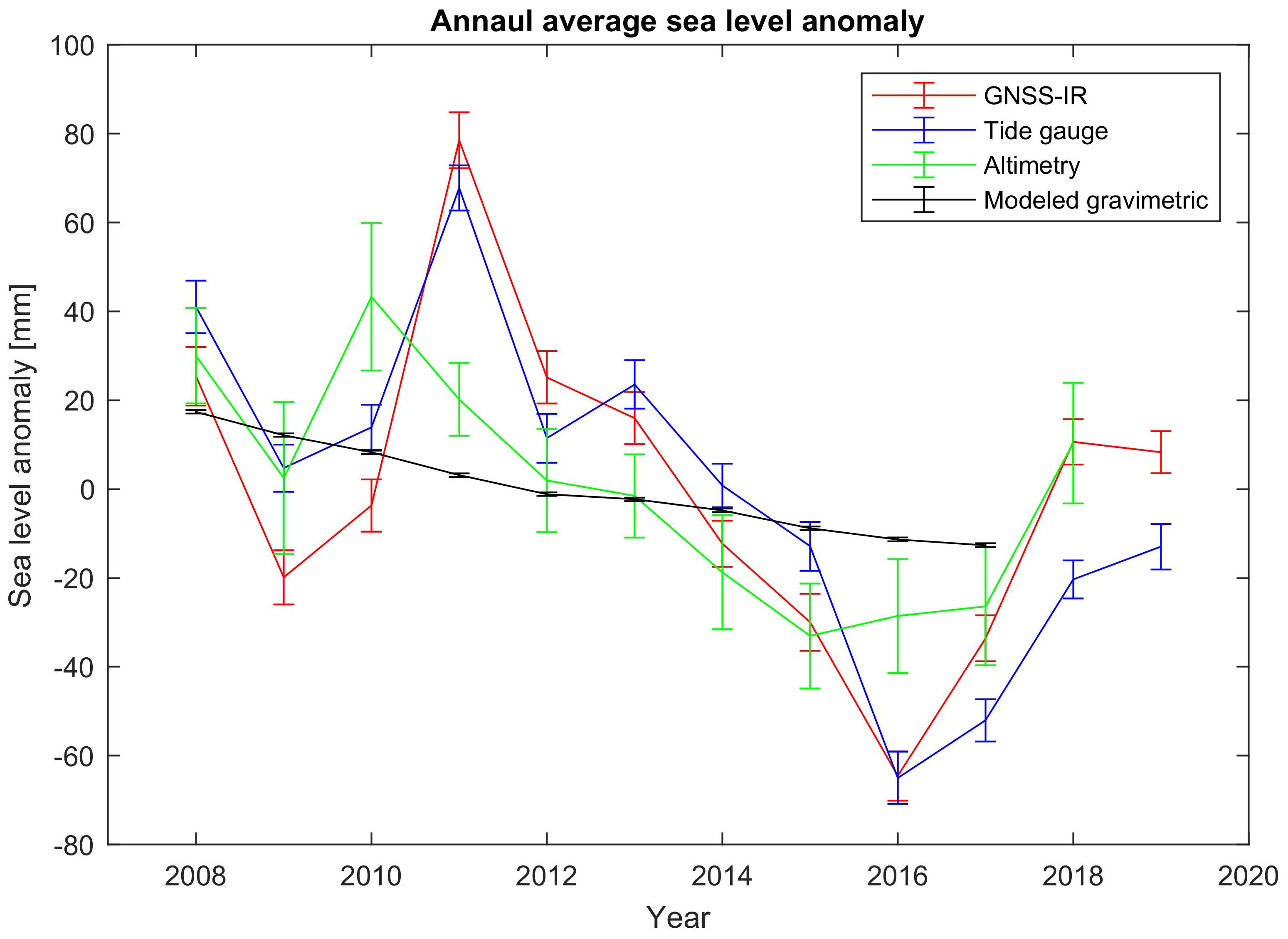
The annual average sea level anomaly using each method is shown in Figure 3. Monthly sea level results from TG, GNSS-IR and altimetry can be found in the supplementary material. Since the TG is not datum controlled, it is not possible to compare the absolute sea level using the three methods. Instead, we compare inter annual changes in the sea level. To directly compare sea level measured using GNSS and TG with altimetry, GNSS-IR and TG results are corrected for vertical land movement as measured by the GNSS station. Since the estimated error on the measured uplift is an order of magnitude smaller than on the sea level and the same vertical uplift correction is done for GNSS-IR and TG sea levels, the error of the uplift measurement is not included in the error bars.
We estimate a linear correlation between annual sea level from GNSS-IR and TG of 0.87. The linear trend in sea level is −4 ± 7 mm/year and −7 ± 5 mm/year for GNSS-IR and TG, respectively. The linear trend in annual sea level measured by altimetry is −5 ± 4 mm/year.
The estimated uncertainty of the annual average sea level measurements using TG and GNSS varies between 4 and 6 mm. The estimated uncertainty of the annual Altimetry results is between 2 and 8 mm and depends strongly on the satellite altimeter used, with considerably larger error estimates for Envisat than for Cryosat-2. It can be seen that though the three timeseries show similar variations they still differ more than would be expected from the estimated measurement errors. The RMSD between annual GNSS-IR and TG sea level changes is 18 mm which is considerably higher than the estimated errors. For the altimetry results, the RMSD with TG and GNSS-IR is 31 and 24 mm, respectively. Deviations larger that the uncertainty is not unexpected between altimetry and the other methods as the TG and GNSS-IR are local measurements, while the sea level from altimetry is calculated over an area off the coast (Figure 2).
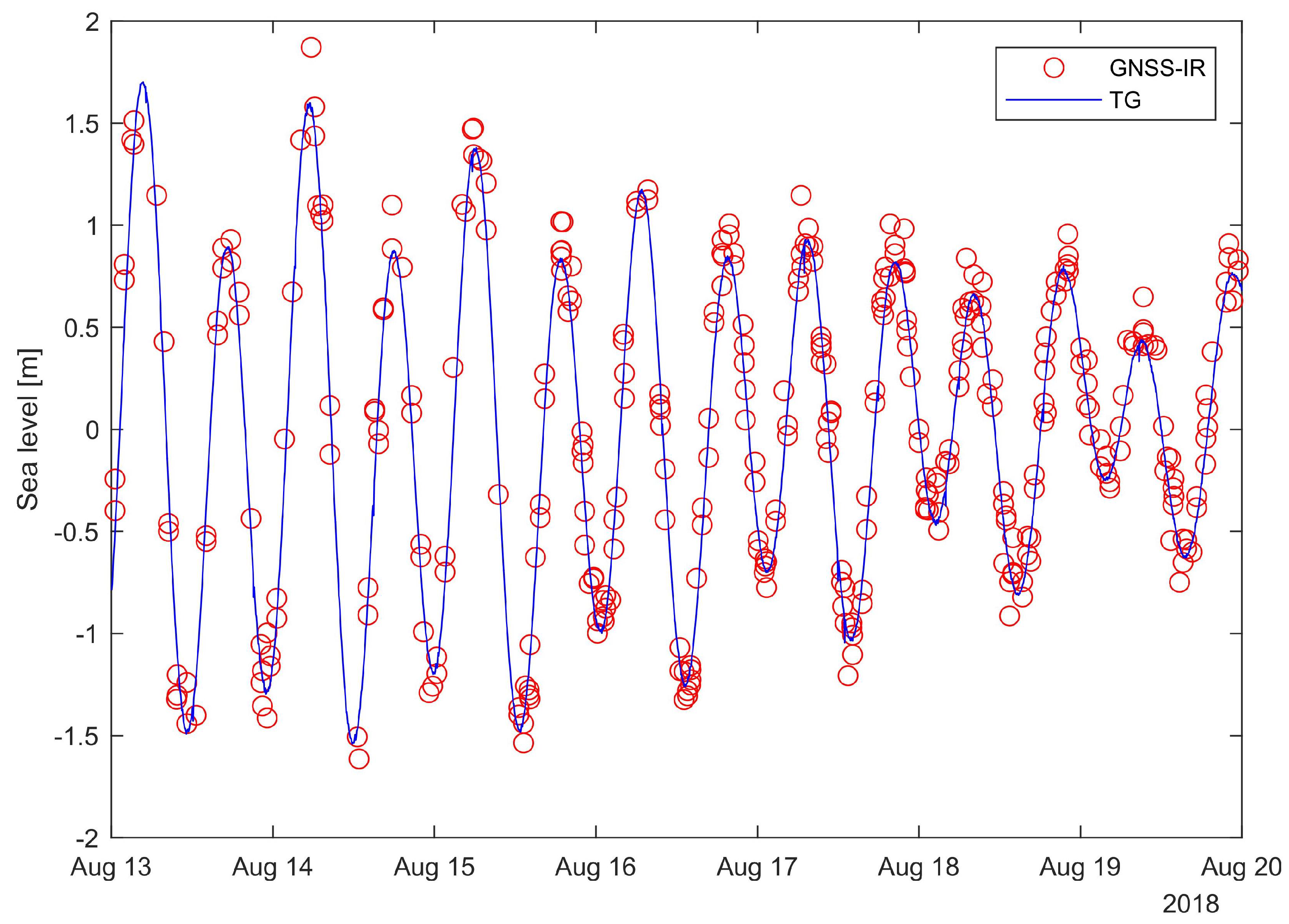
Figure 4 shows one week of sea level variation from August 2018 using GNSS-IR and TG. Note that the TG in Thule is not datum controlled and therefore the mean sea level is subtracted from both time series and the sea level variations compared. The Root Mean Square Deviation (RMSD) of individual measurements of sea level variation is 13 cm for August 2018 which compares well with other spectral SNR studies [5,6]. Figures of individual GNSS-IR measurements for the full year 2018 can be found in the supplementary material. If we instead compare daily values of sea level from GNSS-IR and TG for the whole study period the correlation between the two is 0.84 and the RMS deviation is 65 mm.
Figure 3 also includes the modeled gravity related sea level change. The average gravity related sea level has been altered such that the average is the same as the average of GNSS-IR and TG sea levels over the covered period. The trend in the modeled gravitational sea level is −3 ± 0.4 mm/year while it is −8 ± 9 mm/year and −10 ± 7 mm/year for GNSS-IR and TG, respectively, for this period. The inter annual variations in the gravity related sea level are very small compared to the measured sea level and therefore it is unlikely that the large year-to-year variations are related to gravitational effects. The large year-to-year variations combined with the relatively short timescale also result in large uncertainties on the trends. Thus one should be careful when comparing the trends as the large year-to-year variations will strongly affect the calculated trend.
4. Discussion
We have compared inter annual sea level variations in Thule measured by GNSS-IR, TG and satellite altimetry. We find that the annual variations from GNSS-IR are comparable with those from TG, but that the differences are larger than the estimated errors.
The sea level trends also differ between the three methods but due to high uncertainties on the trends they are within the estimated errors. We expect that the high uncertainties on the trends are a result of the large inter annual variations in the sea level compared to the trend, combined with a relatively short time series when it comes to long term studies.
The standard deviation of the daily GNSS-IR and TG measurements, used to estimate the error, is 110 and 94 mm respectively. For comparison, the RMSD between the two is 65 mm. This indicates that our estimated errors on the two measurements may be too large. This is especially true since the two methods are expected to deviate in winter due to sea ice formation, which introduces a difference that is not a measurement error in traditional terms. If we instead look at the annual averages, the RMSD between TG and GNSS-IR is 18 mm, which is about 4 times the estimated error of the mean. This may seem strange as the RMSD was smaller than the standard deviation for the daily measurements, used to estimate the errors. We expect that this is related to the fact that a considerable part of the difference between the two data sets is not random errors on the individual measurements. These differences will be passed to the means and are not captured by the estimated errors.
The ocean around Thule is covered by sea ice during much of the year and only consistently ice free a couple of months each year. Strandberg et al. [27] show that there are significant changes in the SNR from the GNSS station when sea ice is present. Furthermore, TGs estimate sea level by measuring the pressure at a certain position in the water column while GNSS-IR estimates the distance from GNSS antenna and to the sea surface. Therefore, one source of such non-random deviations could be differences in sea ice cover from year to year, as this would affect the two measurements differently. However, if a similar comparison is done using only data from August and September, where the water is assumed to be ice free, the correlation is 0.69 and the RMSD 37 mm. Thus, the correlation decreases and the RMSD is larger than for the full year average. The increase in RMSD and decrease in correlation is likely due to the use of much less data in total when we limit the mean to this period. However, the RMSD is still large compared to what we would expect from the daily and individual measurements and thus we do not believe that inter annual variations in sea ice alone can explain the differences that we observe.
Other studies comparing sea levels extracted from GNSS-IR with TGs, generally find lower RMSD than we do here. Larson et al. [13] compares GNSS-IR from Kachemak Bay, Alaska, with tide gauge data over one year. They find a RMSD of 23 mm for the daily means. In another study, Larson et al. [6] analyse 10 years of sea level data at Friday Harbor, Washington, and find an RMSD between daily sea levels from GNSS-IR and TG of 21 mm. Both mentioned studies were conducted using one-antenna geodetic GNSS stations, which were installed with the purpose of measuring land motion. Thus, the GNSS equipment used is comparable to the station installed in Thule.
The significant deviations between TG and GNSS-IR may be partly due to the TG not being datum controlled and thus there may be small unknown shifts or drifts in the data series. These could happen at the time of maintenance or be related to changes in the equipment. There have been no changes in the GNSS antenna during the period of interest, but there has been a couple of changes to the TG. The TG sensor was exchanged in 2008, 2015 and 2017. In 2015 the TG was also moved to a different location (Figure 2). On top of this there is an unknown amount of other maintenance jobs which could also disturb the time series as the TG is not datum controlled.
If we compare the sea level from GNSS-IR and TG until 2015 where the TG was moved the RMSD is 13 mm. Though the RMSD on the annual averages are smaller than for the full period it is still large compared to the estimated errors and though the move may explain some of the difference it does not explain all.
The sea level estimates from altimetry differs significantly from both GNSS-IR and TG results. Thus the altimetry does not indicate the source of the discrepancy between the two. The large discrepancies in sea level variations between the local measurements and altimetry in 2010–2011 is likely related to the transition from Envisat to Cryosat-2 measurements during the first half of 2011. Cryosat-2 uses a new Synthetic Aperture Radar altimetric technology, which greatly reduces footprint. This result in an increased amount of data from leads in the sea-ice compared to its pre-decessor, Envisat. As sea level is generally low during the winter season, this causes the altimeter to miss the 2011 peak in sea level.
The modeled gravity related sea level shows a negative trend that is smaller than measured by GNSS-IR and TG but within the uncertainties on these trends. Thus, changes in the gravity field as a result of ice mass changes in the region can explain why we observe a negative sea level trend in Thule. The inter-annual variations, however, are much smaller than what we observe and must be a result of other effects.
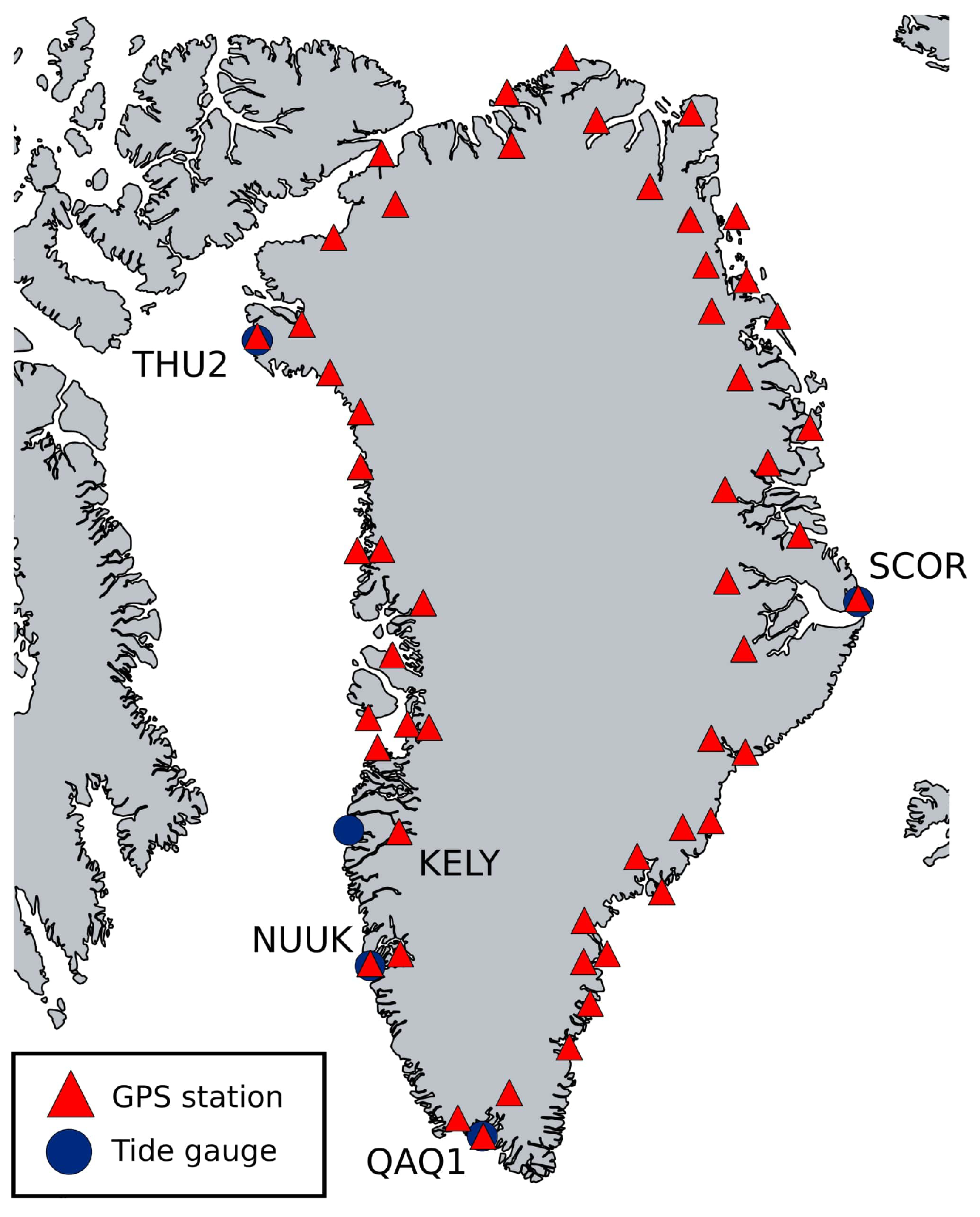
Figure 5 shows a map of all GNET GNSS stations in Greenland as well as TGs with a temporal overlap with the nearest GPS station. There are currently 4 TGs in operation in Greenland: Thule (close to THU2), Scoresbysund (close to SCOR), Godthaab (close to NUUK) and Qaqortoq (close to QAQ1). Unfortunately, neither the Scoresbysund, Nuuk or Qaqortoq GNSS station have a view of the open ocean which is suitable for GNSS-IR purposes. The TG station near KELY was located in Sisimiut but it has not been in operation since 1999. Furthermore, the nearest GNSS station in KELY does not see the open water. Thus, Thule is currently the only place in Greenland where we can directly compare inter annual changes in sea level measured by TG and GNSS-IR.
5. Conclusions
Our results show that the sea level variations measured by GNSS-IR and TG match well on short timescales (Figure 4) and are comparable to other studies. However, there are considerable differences in the inter annual variation that cannot be explained by differences in sea ice cover. We suspect that this difference is related to maintenance on the non-datum controlled TG station. The TG is corrected for uplift using position data from the GNSS station but there may be changes e.g., during maintenance not captured by this. The altimetry differs significantly from both the two local measurements and thus cannot be used to indicate whether one or the other is most representative of the sea level in Thule. Modeled gravity related sea level has a negative trend of −3 ± 0.4 mm/year with only small inter annual variations. We suggest that the GNSS-IR method should be further tested in glaciated areas, preferably against a datum controlled TG.
Since the uncertainty on individual measurements is high [5,28] and the measurement frequency is controlled by the passing of satellites, GNSS-IR cannot replace tide gauges, and should instead be seen as a potential supplement. The technique has the immediate benefit that we have an on-site measurement of vertical land movement and the results can be used directly for studies of eustatic sea level change. This is especially useful in places with large vertical land movements such as glaciated regions and in tectonically active areas.
We suggest that the option of using GNSS stations for sea level monitoring is taken into consideration when installing new GNSS stations in coastal areas and that the stations are installed with an open view of the ocean when feasible.
Supplementary Materials
The following are available online at https://www.mdpi.com/article/10.3390/rs13245077/s1.
Author Contributions
Methodology, T.S.D.-J.; Formal analysis, T.S.D.-J.; data processing, S.D.P.W. (reflectometry) and V.H. (ice heights); writing—original draft preparation, T.S.D.-J.; writing—review and editing, All; visualization, T.S.D.-J.; supervision, S.A.K. and O.B.A. All authors have read and agreed to the published version of the manuscript.
Funding
S.A. Khan, O.B. Andersen and T.S. Dahl-Jensen was funded by the INTAROS GA No. 727890 funded by European Union’s Horizon 2020 Research and Innovation Programme.
Institutional Review Board Statement
Not applicable.
Informed Consent Statement
Not Applicable.
Data Availability Statement
Data sources are referenced in the text. The GNSS data from the station in Thule (THU2) is publicly available from the UNAVCO website (https://www.unavco.org/data/gps-gnss/gps-gnss.html, accessed on 1 December 2021). The mass change data from Antarctica can be downloaded from the Technical University of Dresden (https://data1.geo.tu-dresden.de/ais_gmb/, accessed on 1 December 2021). The ESA CCI DTU/TUM altimetry product is available at https://ftp.space.dtu.dk/pub/ARCTIC_SEALEVEL/DTU_TUM_V3_2019/, accessed on 1 December 2021. The data from the tide gauge in Thule is available at https://ftp.space.dtu.dk/pub/Sealevel/, accessed on 1 December 2021.
Conflicts of Interest
The authors declare no conflict of interest.
References
- Spada, G.; Galassi, G. New estimates of secular sea level rise from tide gauge data and GIA modelling. Geophys. J. Int. 2012, 191, 1067–1094. [Google Scholar] [CrossRef] [Green Version]
- Church, J.; White, N.; Coleman, R.; Lambeck, K.; Mitrovica, J. Estimates of the regional distribution of sea level rise over the 1950–2000 period. J. Clim. 2004, 17, 2609–2625. [Google Scholar] [CrossRef]
- Hsu, C.W.; Velicogna, I. Detection of sea level fingerprints derived from GRACE gravity data. Geophys. Res. Lett. 2017, 44, 8953–8961. [Google Scholar] [CrossRef]
- Woeppelmann, G.; Letetrel, C.; Santamaria, A.; Bouin, M.N.; Collilieux, X.; Altamimi, Z.; Williams, S.D.P.; Miguez, B.M. Rates of sea-level change over the past century in a geocentric reference frame. Geophys. Res. Lett. 2009, 36. [Google Scholar] [CrossRef]
- Lofgren, J.S.; Haas, R.; Scherneck, H.G. Sea level time series and ocean tide analysis from multipath signals at five GPS sites in different parts of the world. J. Geodyn. 2014, 80, 66–80. [Google Scholar] [CrossRef] [Green Version]
- Larson, K.M.; Ray, R.D.; Williams, S.D.P. A 10-Year Comparison of Water Levels Measured with a Geodetic GPS Receiver versus a Conventional Tide Gauge. J. Atmos. Ocean. Technol. 2017, 34, 295–307. [Google Scholar] [CrossRef] [Green Version]
- Strandberg, J.; Hobiger, T.; Haas, R. Improving GNSS-R sea level determination through inverse modeling of SNR data. Radio Sci. 2016, 51, 1286–1296. [Google Scholar] [CrossRef] [Green Version]
- Kim, S.K.; Park, J. Monitoring Sea Level Change in Arctic using GNSS-Reflectometry. In Proceedings of the 2019 International Technical Meeting of the Institute of Navigation, Reston, VA, USA, 28–31 January 2019; pp. 665–675. [Google Scholar] [CrossRef]
- Khan, S.A.; Sasgen, I.; Bevis, M.; van Dam, T.; Bamber, J.L.; Wahr, J.; Willis, M.; Kjaer, K.H.; Wouters, B.; Helm, V.; et al. Geodetic measurements reveal similarities between post-Last Glacial Maximum and present-day mass loss from the Greenland ice sheet. Sci. Adv. 2016, 2, e1600931. [Google Scholar] [CrossRef] [PubMed] [Green Version]
- Bevis, M.; Wahr, J.; Khan, S.A.; Madsen, F.B.; Brown, A.; Willis, M.; Kendrick, E.; Knudsen, P.; Box, J.E.; van Dam, T.; et al. Bedrock displacements in Greenland manifest ice mass variations, climate cycles and climate change. Proc. Natl. Acad. Sci. USA 2012, 109, 11944–11948. [Google Scholar] [CrossRef] [Green Version]
- Tabibi, S.; Geremia-Nievinski, F.; Francis, O.; van Dam, T. Tidal analysis of GNSS reflectometry applied for coastal sea level sensing in Antarctica and Greenland. Remote Sens. Environ. 2020, 248, 111959. [Google Scholar] [CrossRef]
- Williams, S.D.P.; Bell, P.S.; McCann, D.L.; Cooke, R.; Sams, C. Demonstrating the Potential of Low-Cost GPS Units for the Remote Measurement of Tides and Water Levels Using Interferometric Reflectometry. J. Atmos. Ocean. Technol. 2020, 37, 1925–1935. Available online: https://journals.ametsoc.org/jtech/article-pdf/37/10/1925/5010618/jtechd200063.pdf (accessed on 1 December 2021). [CrossRef]
- Larson, K.M.; Ray, R.D.; Nievinski, F.G.; Freymueller, J.T. The Accidental Tide Gauge: A GPS Reflection Case Study From Kachemak Bay, Alaska. IEEE Geosci. Remote Sens. Lett. 2013, 10, 1200–1204. [Google Scholar] [CrossRef] [Green Version]
- Williams, S.D.P.; Nievinski, F.G. Tropospheric delays in ground-based GNSS Multipath Reflectometry— Experimental evidence from coastal sites. J. Geophys. Res. Solid Earth 2017, 122, 2310–2327. [Google Scholar] [CrossRef] [Green Version]
- Rose, S.K.; Andersen, O.B.; Passaro, M.; Ludwigsen, C.A.; Schwatke, C. Arctic Ocean Sea Level Record from the Complete Radar Altimetry Era: 1991–2018. Remote Sens. 2019, 11, 1672. [Google Scholar] [CrossRef] [Green Version]
- Andersen, O. Shallow water tides in the northwest European shelf region from TOPEX/POSEIDON altimetry. J. Geophys. Res.-Ocean. 1999, 104, 7729–7741. [Google Scholar] [CrossRef]
- Khan, S.A.; Wahr, J.; Leuliette, E.; van Dam, T.; Larson, K.M.; Francis, O. Geodetic measurements of postglacial adjustments in Greenland. J. Geophys. Res.-Solid Earth 2008, 113. [Google Scholar] [CrossRef] [Green Version]
- Wang, H.; Xiang, L.; Jia, L.; Jiang, L.; Wang, Z.; Hu, B.; Gao, P. Load Love numbers and Green’s functions for elastic Earth models PREM, iasp91, ak135, and modified models with refined crustal structure from Crust 2.0. Comput. Geosci. 2012, 49, 190–199. [Google Scholar] [CrossRef]
- Groh, A.; Horwath, M. The method of tailored sensitivity kernels for GRACE mass change estimates. Geophys. Res. Abstr. 2016, 18, EGU2016-12065. [Google Scholar]
- Krabill, W. IceBridge ATM L2 Icessn Elevation, Slope, and Roughness, [1994–2010]; National Snow and Ice Data Center: Boulder, CO, USA, 2011. [Google Scholar]
- Zwally, H.J.; Schutz, R.; Bentley, C.; Bufton, J.; Herring, T.; Minster, J.; Spinhirne, J.; Thomas, R. GLAS/ICESat L2 Antarctic and Greenland Ice Sheet Altimetry Data, Version 34; Indicate Subset Used; NASA National Snow and Ice Data Center: Boulder, CO, USA, 2014. [Google Scholar] [CrossRef]
- Helm, V.; Humbert, A.; Miller, H. Elevation and elevation change of Greenland and Antarctica derived from CryoSat-2. Cryosphere 2014, 8, 1539–1559. Available online: https://tc.copernicus.org/articles/8/1539/2014/tc-8-1539-2014.pdf (accessed on 1 December 2021). [CrossRef] [Green Version]
- Khan, S.A.; Kjaer, K.H.; Korsgaard, N.J.; Wahr, J.; Joughin, I.R.; Timm, L.H.; Bamber, J.L.; van den Broeke, M.R.; Stearns, L.A.; Hamilton, G.S.; et al. Recurring dynamically induced thinning during 1985 to 2010 on Upernavik Isstrom, West Greenland. J. Geophys. Res.-Earth Surf. 2013, 118, 111–121. [Google Scholar] [CrossRef] [Green Version]
- Marzeion, B.; Jarosch, A.H.; Hofer, M. Past and future sea-level change from the surface mass balance of glaciers. Cryosphere 2012, 6, 1295–1322. [Google Scholar] [CrossRef] [Green Version]
- RGI Consortium. Randolph Glacier Inventory—A Dataset of Global Glacier Outlines: Version 6.0. In Global Land Ice Measurements from Space; Technical Report; Digital Media: Denver, CO, USA, 2017. [Google Scholar] [CrossRef]
- Khan, S.A.; Kjaer, K.H.; Bevis, M.; Bamber, J.L.; Wahr, J.; Kjeldsen, K.K.; Bjork, A.A.; Korsgaard, N.J.; Stearns, L.A.; van den Broeke, M.R.; et al. Sustained mass loss of the northeast Greenland ice sheet triggered by regional warming. Nat. Clim. Chang. 2014, 4, 292–299. [Google Scholar] [CrossRef]
- Strandberg, J.; Hobiger, T.; Haas, R. Coastal Sea Ice Detection Using Ground-Based GNSS-R. IEEE Geosci. Remote. Sens. Lett. 2017, 14, 1552–1556. [Google Scholar] [CrossRef]
- Larson, K.M.; Lofgren, J.S.; Haas, R. Coastal sea level measurements using a single geodetic GPS receiver. Adv. Space Res. 2013, 51, 1301–1310. [Google Scholar] [CrossRef] [Green Version]
Figure 1.
Illustration of the three methods used for measuring sea level in Thule in this study.

Figure 2.
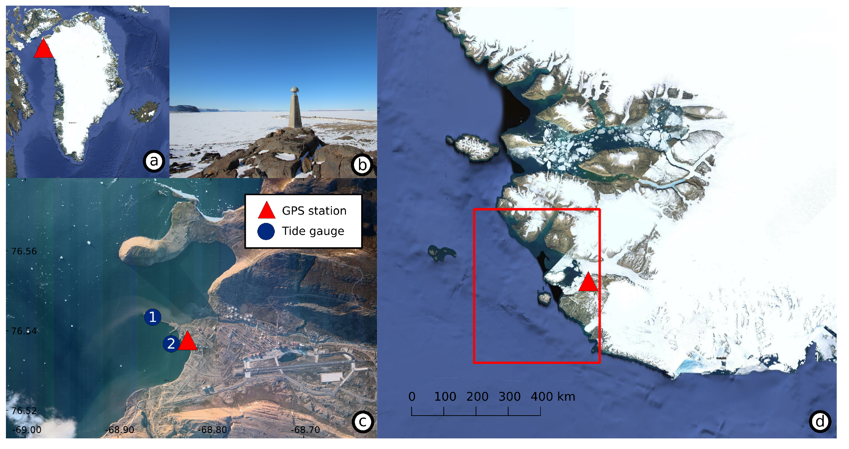
Maps illustrating the study area. (a) Map of Greenland. Thule is marked by the red triangle. (b) Picture of the GNSS station in Thule with the view over the ocean. (c) Map of Thule with GNSS- and TG station locations. 1 marks the position of the TG until September 2015 and 2 marks the position since then. (d) The red rectangle illustrates the area used for sea level extraction from altimetry.
Figure 2.
Maps illustrating the study area. (a) Map of Greenland. Thule is marked by the red triangle. (b) Picture of the GNSS station in Thule with the view over the ocean. (c) Map of Thule with GNSS- and TG station locations. 1 marks the position of the TG until September 2015 and 2 marks the position since then. (d) The red rectangle illustrates the area used for sea level extraction from altimetry.

Figure 3.
Annual average sea level change at Thule using GNSS-IR, TG and altimetry. The error bars illustrate the annual standard deviation of the mean as described in Section 2. The figure also includes variations in the modeled gravity related sea level.
Figure 3.
Annual average sea level change at Thule using GNSS-IR, TG and altimetry. The error bars illustrate the annual standard deviation of the mean as described in Section 2. The figure also includes variations in the modeled gravity related sea level.

Figure 4.
Individual measurements of sea level variation using GNSS Interferometric Reflectometry (GNSS-IR) and Tide Gauge (TG) from one week in August 2018 (13 to 19 of August).
Figure 4.
Individual measurements of sea level variation using GNSS Interferometric Reflectometry (GNSS-IR) and Tide Gauge (TG) from one week in August 2018 (13 to 19 of August).

Figure 5.
Map of Greenland with indication of GNET GNSS stations and tide gauges with data overlapping the nearest GPS station.
Figure 5.
Map of Greenland with indication of GNET GNSS stations and tide gauges with data overlapping the nearest GPS station.

Publisher’s Note: MDPI stays neutral with regard to jurisdictional claims in published maps and institutional affiliations. |
© 2021 by the authors. Licensee MDPI, Basel, Switzerland. This article is an open access article distributed under the terms and conditions of the Creative Commons Attribution (CC BY) license (https://creativecommons.org/licenses/by/4.0/).
Share and Cite
MDPI and ACS Style
Dahl-Jensen, T.S.; Andersen, O.B.; Williams, S.D.P.; Helm, V.; Khan, S.A. GNSS-IR Measurements of Inter Annual Sea Level Variations in Thule, Greenland from 2008–2019. Remote Sens. 2021, 13, 5077. https://doi.org/10.3390/rs13245077
AMA Style
Dahl-Jensen TS, Andersen OB, Williams SDP, Helm V, Khan SA. GNSS-IR Measurements of Inter Annual Sea Level Variations in Thule, Greenland from 2008–2019. Remote Sensing. 2021; 13(24):5077. https://doi.org/10.3390/rs13245077
Chicago/Turabian StyleDahl-Jensen, Trine S., Ole B. Andersen, Simon D. P. Williams, Veit Helm, and Shfaqat A. Khan. 2021. "GNSS-IR Measurements of Inter Annual Sea Level Variations in Thule, Greenland from 2008–2019" Remote Sensing 13, no. 24: 5077. https://doi.org/10.3390/rs13245077
Note that from the first issue of 2016, this journal uses article numbers instead of page numbers. See further details here.