
Developing and Testing a Deep Learning Approach for Mapping Retrogressive Thaw Slumps


1
Alfred Wegener Institute Helmholtz Centre for Polar and Marine Research, 14473 Potsdam, Germany
2
Remote Sensing Technology Institute (IMF), German Aerospace Center (DLR), 82234 Weßling, Germany
3
Data Science in Earth Observation, Technical University of Munich (TUM), 80333 Munich, Germany
4
Institute of Geosciences, University of Potsdam, 14476 Potsdam, Germany
*
Author to whom correspondence should be addressed.
Remote Sens. 2021, 13(21), 4294; https://doi.org/10.3390/rs13214294
Submission received: 22 September 2021
/
Revised: 8 October 2021
/
Accepted: 11 October 2021
/
Published: 26 October 2021
(This article belongs to the Special Issue Dynamic Disturbance Processes in Permafrost Regions)
Abstract
:In a warming Arctic, permafrost-related disturbances, such as retrogressive thaw slumps (RTS), are becoming more abundant and dynamic, with serious implications for permafrost stability and bio-geochemical cycles on local to regional scales. Despite recent advances in the field of earth observation, many of these have remained undetected as RTS are highly dynamic, small, and scattered across the remote permafrost region. Here, we assessed the potential strengths and limitations of using deep learning for the automatic segmentation of RTS using PlanetScope satellite imagery, ArcticDEM and auxiliary datasets. We analyzed the transferability and potential for pan-Arctic upscaling and regional cross-validation, with independent training and validation regions, in six different thaw slump-affected regions in Canada and Russia. We further tested state-of-the-art model architectures (UNet, UNet++, DeepLabv3) and encoder networks to find optimal model configurations for potential upscaling to continental scales. The best deep learning models achieved mixed results from good to very good agreement in four of the six regions (maxIoU: 0.39 to 0.58; Lena River, Horton Delta, Herschel Island, Kolguev Island), while they failed in two regions (Banks Island, Tuktoyaktuk). Of the tested architectures, UNet++ performed the best. The large variance in regional performance highlights the requirement for a sufficient quantity, quality and spatial variability in the training data used for segmenting RTS across diverse permafrost landscapes, in varying environmental conditions. With our highly automated and configurable workflow, we see great potential for the transfer to active RTS clusters (e.g., Peel Plateau) and upscaling to much larger regions.
1. Introduction
The changing climate of the Arctic, with both measured and projected air temperatures and precipitation rapidly increasing [1,2], has a significant impact on permafrost [3,4,5]. As permafrost soils store about twice the amount of carbon as that found in the atmosphere [6,7], permafrost thaw and resulting carbon feedbacks are expected to have a significant impact on the global climate [8]. Rising permafrost ground temperatures have been observed across almost the entire Arctic permafrost region [3]. As a result of warming, permafrost becomes more vulnerable to disturbances of [9] and degradation in ground ice-rich landscapes due to thermokarst and thermo-erosion.
Retrogressive thaw slumps (RTS) are typical landforms related to processes of rapidly thawing and degrading hillslope permafrost [10]. Although these mass-wasting processes have been observed in different Arctic regions in the past decades [11,12,13], many recent field and remote sensing studies found increasing occurrence and faster progression in various permafrost regions [12,14,15,16,17,18].
As RTS typically have a small size (<10 ha, with a few exceptions reaching up to ~1 km²), as well as a wide range of appearances and dynamics, their detection and monitoring on the regional to continental scale would require globally available imagery at sufficiently high spatial and temporal resolutions. Their formation is bound to specific environmental and permafrost conditions, such as ice-rich permafrost and sloped terrains [10,12,19], thus limiting their presence to regional clusters. Particularly, regions with massive amounts of buried ice, as preserved in the moraines of former glaciations [17,20,21], or regions with thick syngenetic ice-wedges in yedoma permafrost [22,23], or with very fine grained marine deposits that were raised above sea level following deglaciation and thus formed very icy epigenetic permafrost, can be prone to RTS development [18]. Furthermore, increasing temperatures and precipitation have likely caused the increased formation and growth of RTS [21,24].
Fairly well-studied regions for the occurrence of thaw slumps are typically clustered and located in former ice-marginal regions of the Laurentide Ice Sheet in NW Canada, most notably the Peel Plateau [17,21] and Banks Island [16], or moraines of formerly glaciated mountain ranges, e.g., the Brooks Range in northern Alaska [20,25]. Intensively studied regions in Siberia include the Yamal Peninsula [13,26], Kolguev Island [27], Bolshoy Lyakhovsky Island [22] and the Yana Basin with its famous Batagaika mega slump [14,28]. However, the latter is, atypically, not part of a larger cluster of RTS. The total quantity and distribution of RTS in the Arctic remains unknown.
Several remote sensing studies have used very high-resolution (VHR) satellite data, but RTS are typically delineated manually, which is a labor-intensive task and therefore prohibitive for larger regions. The use of airborne [29,30] or UAV data [31] to survey small areas with RTS is becoming more popular. These datasets allow for the creation of elevation data and multiple observations, thus providing a basis for more automated approaches [29,30,31]. Highly automated approaches, which will be required to map RTS across larger regions and multiple time steps, are fairly scarce so far. Nitze et al. [32] used a random forest machine learning approach to map RTS and other permafrost disturbances, such as lake dynamics and wildfire, on Landsat data across four large north–south transects in the Arctic covering ~2.2 million km2. For the indirect detection of RTS and thaw-related erosion features, Lara et al. [33] measured changes in lake color as a proxy for rapid thermo-erosion dynamics in a watershed-scale study in NW Alaska using Landsat. However, the coarse resolution of Landsat (30 m) proved to be a highly limiting factor in detecting RTS features accurately [32]. A combination of Landsat and Sentinel-2 imagery was used to assess RTS dynamics with the LandTrendr disturbance detection algorithm over a ~8 million km2 region of East Siberia for a 20-year period from 2000 to 2019 [34].
Automated approaches applied to higher-resolution data (better than 5 m ground resolution), such as high-resolution RapidEye and PlanetScope imagery or very high-resolution DigitalGlobe/Maxar imagery, pose specific challenges for image classification and specifically object detection. On such data, pixel-based approaches are no more feasible, and object-based image approaches (OBIA) need to be applied [35]. Traditionally, this has been accomplished with the segmentation followed by classification of image objects. Over the past few years, deep learning (DL) techniques have grown in popularity for object detection or segmentation in imagery of any kind, e.g., bio-medical images or everyday photography.
In remote sensing, DL approaches are also growing in popularity [36] for typical applications such as image segmentation and classification, due to their ability to take spatial context into account. This includes, e.g., the mapping of landslides [37,38,39]. Furthermore, DL-based image segmentation has been particularly applied on VHR data, such as Worldview, GeoEye, etc., to automatically detect comparably small objects, such as buildings [40,41,42] or individual trees [43]. Due to many DL algorithms, such as Mask R-CNN, requiring a fixed amount of input bands, e.g., one or three, and to avoid overfitting, several studies have focused on input band selection and optimization [44,45,46].
In permafrost remote sensing, deep learning applications are very scarce so far. They have been applied for mapping and segmenting ice-wedge polygons [47,48,49] and for detecting infrastructure across the Arctic permafrost region [50]. DL for detecting and tracking RTS was used by Huang et al. [51,52], who tested the applicability of the DeepLabv3+ DL architecture for detecting and monitoring RTS on the Tibetan Plateau using Planet data. They received a high detection quality similar to manual digitization [52], which enabled them to track RTS in space and time within a confined region.
Based on these promising achievements, we here aim to:
(1) test the feasibility of applying DL methods on PlanetScope and auxiliary data to detect and map RTS across different Arctic permafrost regions;
(2) identify the particular advantages and challenges;
(3) discuss the further requirements for using AI-based techniques to eventually map RTS across the circum-Arctic permafrost zone.
2. Materials and Methods
2.1. Study Regions
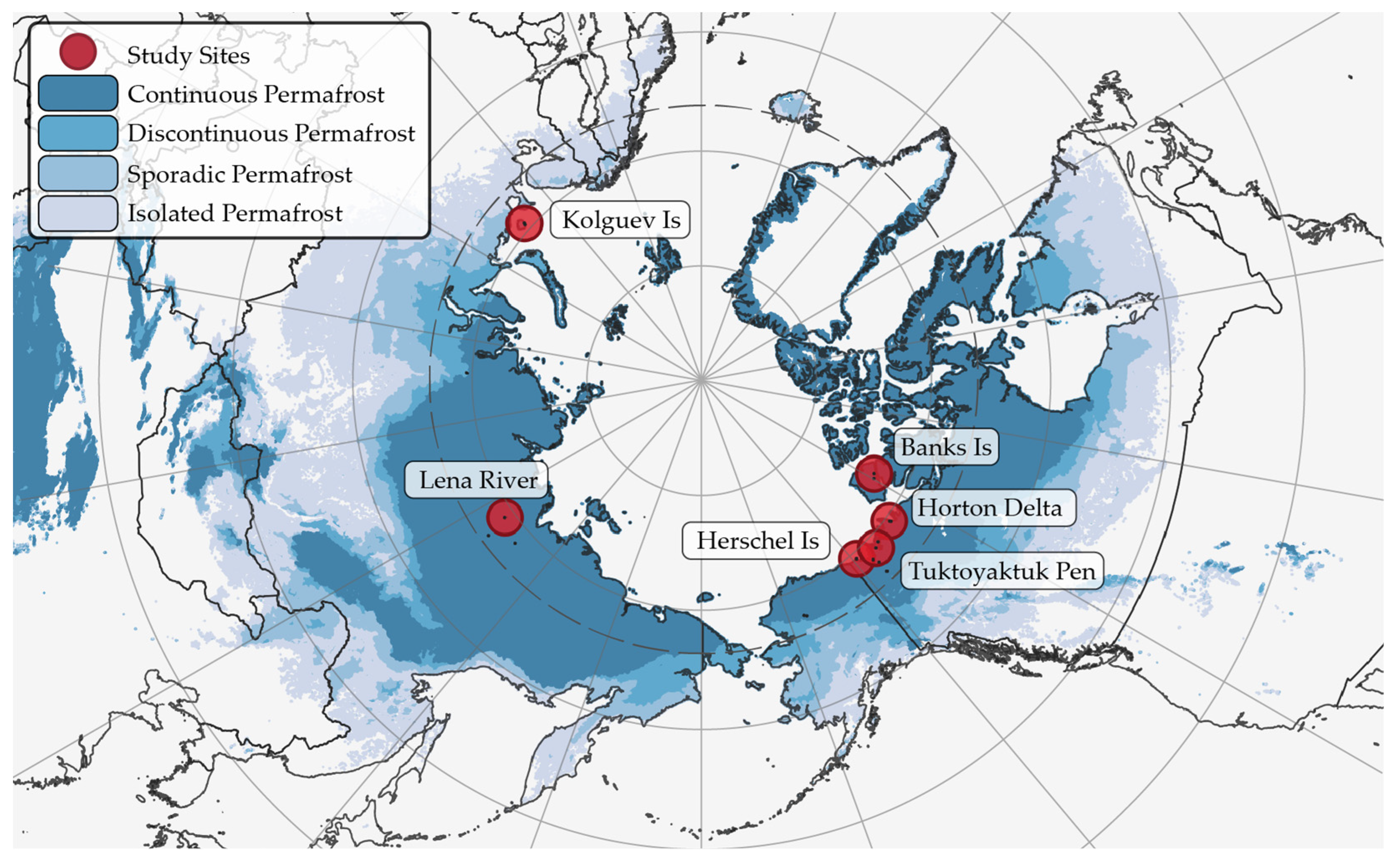
We selected six different sites across the Arctic in Canada and Russia that are affected by RTS (Figure 1; Table 1). These locations were chosen to contain a sufficient number of RTS, and to represent a broad variety of environmental conditions (sparse tundra to taiga) and geographic settings (RTS at coast, river, or lake shores, hillslopes, and moraines). Study sites with a spatially extensive occurrence of RTS (e.g., Horton Delta, Banks Island, Kolguev Island) were each split into two subsets. All sites/subsets have an area of 100 km² (10 × 10 km) to ensure the best possible comparison and normalization to each other.
2.1.1. Banks Island
The Banks Island study site consists of two subsets and is located in the eastern RTS-rich part of Banks Island in NW Canada (see Figure A1 and Figure A2). This region is characterized by glacial moraine deposits (Jesse Moraine) of the former Laurentide Ice Sheet, which contains buried massive ground ice [16,53]. The region is subject to massive permafrost degradation as indicated by strong ice-wedge degradation [54] and abundant RTS [16], which mostly form along lake shores and valley slopes. The vegetation is sparse tundra according to the Circum-Arctic Vegetation Map (CAVM) subzone C [55]. The selected site has some of the largest and most active RTS known globally (see Figure A1d). The region has rolling terrain with an abundance of lakes and river valleys. Modeled ground temperatures are −14 to −15 °C [56].
2.1.2. Herschel Island
This study site covers large parts of Herschel Island in NW Canada (see Figure A3). The Herschel Island site contains large highly active RTS, which have been frequently studied over the past decade [12,57]. Similar to many other RTS-rich sites in NW Canada, Herschel Island is located along the margins of the Laurentide Ice Sheet. The substrate is dominated by permafrost with massive buried glacial ice remnants [58]. The vegetation is dominated by shrubby tundra (erect dwarf shrub tundra) of CAVM Zone E [55]. Due to the rolling hilly nature of the island, there are many small stream catchments, but only a few smaller lakes and ponds. Thaw slumps are predominantly located on the SE shore. Modeled ground temperatures are −5 to −6 °C [56].
2.1.3. Horton Delta
This study site consists of two subsets and is located just south of the Horton River delta in NW Canada at a steep cliff on the Beaufort Sea coast (see Figure A4 and Figure A5). This region was located at the front of a Laurentide Ice Sheet lobe and is known to be affected by RTS [21]. The site is characterized by rolling terrain with steep coastal cliffs and partially deeply incised valleys. Vegetation here is classified as dwarf shrub tundra of CAVM subzone D/E [55]. Lakes are very sparse, but larger valleys with rivers are present within this site. Thaw slumps are predominantly located on top of the coastal cliffs. Smaller RTS are also found along steep valley slopes in close proximity to the coast. Modeled ground temperatures are −7 to −8 °C [56].
2.1.4. Kolguev Island
Kolguev is an island off the coast of Arctic European Russia. It is characterized by ice-rich permafrost with tabular ice [27]. Vegetation here is dominated by Tundra of CAVM Zone D [55]. The study site has a rolling terrain with steep coastal bluffs. RTS are most abundant on these coastal bluffs in the NW of the island. Lakes are very sparse in this region (see Figure A6 and Figure A7). Modeled ground temperatures are 0 to 1 °C [56], though the presence of RTS and therefore ground-ice suggests lower temperatures.
2.1.5. Lena River
This study site is located in the lower reaches of the Lena River on the east side of the river close to the foothills west of the Verkhoyansk Mountain Range in northeastern Siberia. This site is likely a terminal moraine of an ancient outlet glacier from the mountain range, which underwent several glaciations during the Quaternary period [59]. The glacial history of this region is not documented in detail. Vegetation here is boreal forest, and the region is lake-rich. RTS typically formed along the lake’s shores. Former stabilized RTS are also abundant and mostly covered by dense shrubs (see Figure A8). The presence of RTS in this region is only sparsely documented in the literature [32]. Modeled ground temperatures are −7 to −8 °C [56].
2.1.6. Tuktoyaktuk Peninsula
This region is located on the Tuktoyaktuk Peninsula in NW Canada. It is a rolling, glacially (Laurentide Ice Sheet) shaped lowland with massive ground ice [19,60]. The vegetation here is shrubby tundra of CAVM Zone E [55] close to the tundra–taiga ecotone. This region has a large abundance of lakes [61,62]. Thaw slumps typically form along lake shores (see Figure A9). Modeled ground temperatures are −6 to −7 °C [56].
2.2. Data
For training data collection, as well as model training, validation and inference, we used a variety of data. Our primary data source was the PlanetScope [63] multispectral optical data for the years 2018 and 2019. We further used additional datasets, such as the ArcticDEM [64] and Tasseled Cap Landsat Trends [32]. Furthermore, for collecting ground truth, we additionally used the ESRI and Google Satellite layers.
2.2.1. PlanetScope
We used PlanetScope satellite images [63] as our primary data source. PlanetScope data are acquired by a constellation of more than 120 satellites in orbit. They have a spatial resolution of 3.15 m and four spectral bands in the visual (red, green, blue; RGB) and near-infrared (NIR) wavelengths. The high number of satellites in orbit allows for sub-daily temporal resolution, particularly at high-latitudes, where data overlap becomes increasingly dense for satellites following a polar orbit [65]. However, non-obstructed views of the ground are severely limited, particularly in high-latitude coastal regions, due to persistent cloud cover and cloud shadows, haze, and long snow periods. Furthermore, the generally low sun elevations in high-latitude environments can lead to low signal-to-noise ratios.
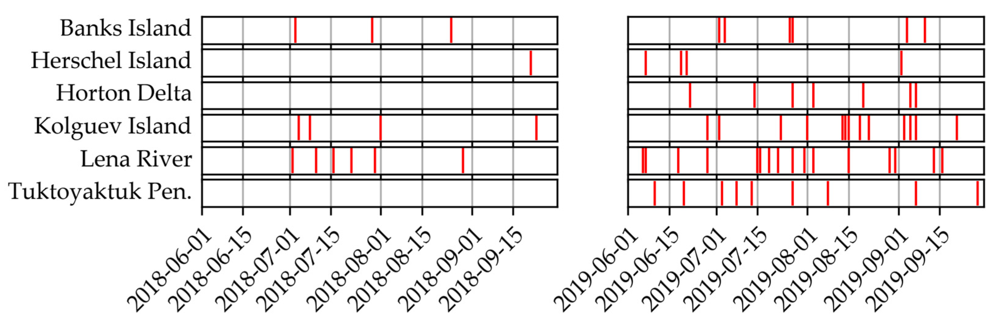
For data selection, we applied the following selection criteria: maximum 10% cloud cover, 90% area coverage, and an observation period from 1 June until 30 September during the years 2018 and 2019. Furthermore, we selected image dates by visual inspection to ensure consistent temporal sampling, where possible. As cloud-free periods (the main limiting factor) tended to be temporally clustered, we omitted several clear sky image dates within short periods (e.g., five consecutive days with clear skies), as these will not provide additional value for training the model. The image dates and IDs are indicated in Figure 2 and Supplementary Table S1. Due to further satellite launches, the number of PlanetScope images increased significantly over our observation period. Thus, available imagery was rather sparse before 2019, but became increasingly abundant after that.
Finally, we downloaded data through the porder download program [66] and Planet Explorer interface. We chose the “analytic_sr,udm2” bundle, which includes surface reflectance data, udm (unusable data mask), udm2 and metadata files. We chose to clip output data automatically to the respective AOI extents, which allowed us to optimize the allocated data quota and to ensure the completeness of all ground truth datasets. Finally, we calculated the Normalized Difference Vegetation Index (NDVI) for each scene as an additional input layer. We used the udm2 data mask to mask out remaining clouds, shadows and snow/ice in the PlanetScope and all auxiliary datasets.
2.2.2. Arctic DEM
We used the ArcticDEM [64] (version 3, Google Earth Engine Dataset: “UMN/PGC/ArcticDEM/V3/2m_mosaic”) to calculate slope and detrended elevation data. The ArcticDEM is available for all land areas north of 60° latitude, but contains minor data gaps.
We calculated the relative (detrended) elevation by subtracting the mean elevation within a circular window (structuring element) with a diameter of 50 pixels (100 m). The relative elevation was used to determine the local pixel position within the surroundings and to remove the influence of the regional elevation. Finally, we rescaled the relative elevation values with an offset of 50 and factor of 300 to minimize the size of data of the unsigned Integer16 type. Furthermore, we calculated the slope in degrees. For both calculations we used the ee.Terrain.slope function in the Google Earth Engine (GEE).
We downloaded the data (relative elevation and slope) for the training sites (buffered by 5 km) from GEE with the native projection (NSIDC Sea Ice Polar Stereographic North, EPSG: 3413) and a spatial resolution of 2 m. We chose GEE over the original data portal due to the simpler accessibility of data, as well as its capacity for slope calculation and process automation. After downloading, all individual tiles were merged into virtual mosaics using gdalbuildvrt to simplify data handling and permit efficient data storage. We later reprojected both datasets, elevation and slope, to the projection, spatial resolution and image extent of individual PlanetScope scenes using gdalwarp within our automated processing pipeline (see Figure 3).
2.2.3. TCVIS
To introduce a decadal-scale multi-temporal dataset into the analysis, we used the temporal trend datasets of Tasseled Cap indices of Landsat data (Collection 1, Tier 1, Surface Reflectance), based on previous work [67,68]. For the period from 2000 to 2019, we filtered Landsat data to scenes with a cloud cover of less than 70% and masked clouds, shadows and snow/ice based on available masking data.
We calculated the Tasseled Cap indices [69], brightness (TCB), greenness (TCG), and wetness (TCW) for each individual scene. Then we calculated the linear trend for each index over time, scaled to 10 years. Finally, we truncated the slope values of all three indices to a range of −0.12 to 0.12 and transformed the data to an unsigned integer data range (0 to 255) to minimize storage use. The resulting data were stored as a publicly readable GEE ImageCollection asset (“users/ingmarnitze/TCTrend_SR_2000-2019_TCVIS”).
2.3. Methods
2.3.1. Slump Digitization
We created ground truth datasets for training and validation by manual digitization in QGIS 3.10 [70]. We used the individual PlanetScope scenes (see Section 2.2.1) as the primary data source. We digitized each available image individually. Accordingly, we have multi-temporal information of RTS in all study regions. The same physical RTS may have different polygon shapes on different dates due to the physical change of the RTS (e.g., growth), presence of snow, its location on the edge of the imagery, geolocation inaccuracies, or slightly inconsistent digitization (see below).
Furthermore, we used auxiliary data to better understand landscape morphology and landscape dynamics, when interpreting potential RTS features. These auxiliary data are the ArcticDEM and multitemporal TCVIS (Landsat Tasseled Cap Trend) data, streamed through the Google Earth Engine Plugin (https://github.com/gee-community/qgis-earthengine-plugin, v0.0.2) in QGIS. Furthermore, additional VHR imagery publicly available in ESRI and Google satellite base layers was accessed and used for mapping through the QuickMapServices Plugin in QGIS [71]. The VHR imagery was used solely for guidance in order to better identify the ground objects at a higher resolution than the 3 m PlanetScope imagery.
Labeling went through two iterations to ensure the highest data quality. In the first step, a trained person manually digitized potential thaw slumps that matched selected criteria. During this iteration, unclear cases were discussed with a second trained person. The criteria for manually outlining RTS in the data were:
- little or no vegetation, surrounded by vegetation;
- presence of a headwall;
- “blue” signature of TCVIS layer, a transition from vegetation to wet soil;
- visible depression in ArcticDEM and derived slope dataset;
- visible thaw slump disturbance in VHR imagery;
- snow was considered as not being part of the RTS.
In the next step the second person checked each individual thaw slump object and confirmed, edited, removed or added new polygons. In this procedure, we closely follow the RTS digitizing guidelines set out by Segal et al. [72].
Although the datasets went through several iterations, oftentimes it was challenging to determine whether the slumps were still active or already stabilized, and therefore whether they needed to be included in or excluded from the process. Furthermore, while actively eroding upper parts of thaw slumps were easy to delineate due to the presence of a headwall, the lower scar zone and debris tongues were typically more challenging to delineate due to unclear boundaries. Overall we digitized 2172 thaw slump polygons. Please find more details in Table 2. The digitized polygons are made freely accessible (see Data Availability Statement).
2.3.2. Deep Learning Model
General Setup
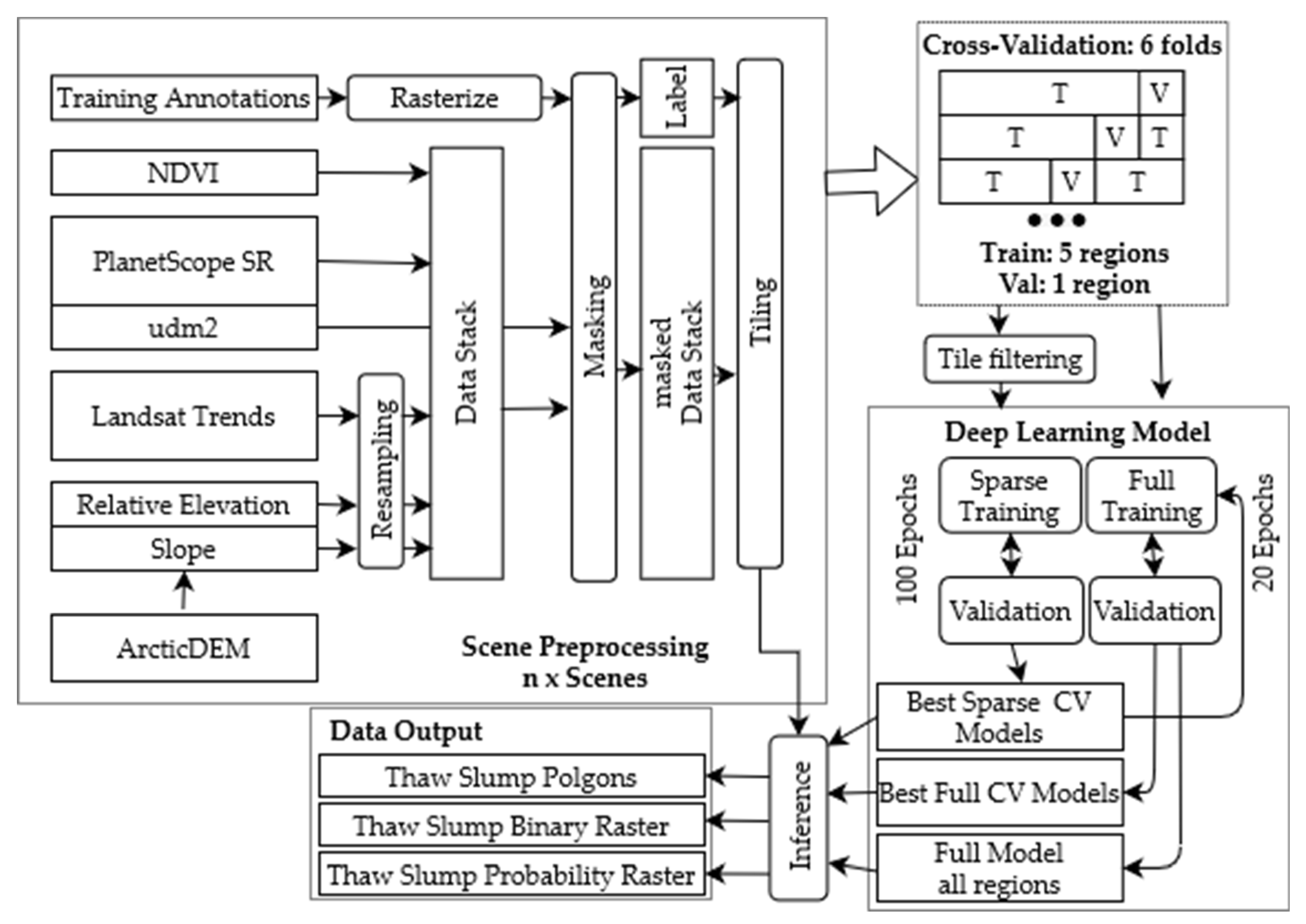
For the data preprocessing, model training, validation, and inference we developed a highly automated processing pipeline to ensure the highest possible level of automation, reproducibility and transferability (see Figure 3). It is easily configurable with configuration files, which allow us to define the key processing parameters, such as dataset (train, val, test), data sources (see Table 3), DL model architecture and encoder, model depth, and many more. Our processing chain is based on the pytorch deep learning framework [73] within the python programming language. Furthermore, we relied on several additional packages for specific tasks (see below).
The processing was split into three main steps: first, data preprocessing; second, model training and validation; third, model inference.
The code is tracked and documented in a git repository (see code). We used version 0.4.1 for the training and validation. We performed the inference on version 0.5.2, which included bug fixes related to inference, compared to version 0.4.1.
Hardware
We ran our model training and inference on virtual machines equipped with a shared and virtualized NVIDIA GV100GL GPU (Tesla V100 PCIe 32 GB). The VM was allocated with 16 GB GPU RAM, 8x Intel(R) Xeon(R) Gold 6230 CPU, 128 GB RAM and fast storage.
Augmentation
In order to increase its size and to introduce more variety into the training dataset, the input imagery was augmented in several ways. Since satellite imagery is largely independent of orientation, the images were randomly mirrored along their horizontal and vertical axes, as well as being rotated by multiples of 90°. Randomly blurring some input images during training further improved model robustness. Augmentation increased the training set size eight-fold. Image augmentation was conducted and implemented using the Albumentations python library [74]. Each augmentation type was randomly applied with a probability of 50% per image.
Model Architecture
For the pixel-wise classification of images, semantic segmentation models offer an efficient approach to combining local information and contextual clues. For our model architecture we evaluated some network architectures commonly used for semantic segmentation. These segmentation architectures consist of an encoder network and a decoder. Successful image classification architectures are commonly used as encoders, as these can efficiently extract general image features. Therefore, we evaluated three ResNet [75] architectures (Resnet34, Resnet50 and Resnet101) as possible encoders for our network. Decoders are currently undergoing the most innovation in semantic segmentation, and thus vary a lot from architecture to architecture. Here, we evaluated three approaches, namely, UNet [76], UNet++ [77] and DeepLabv3 [78]. The model architectures are based on the implementation of the segmentation_models_pytorch package (https://github.com/qubvel/segmentation_models.pytorch, v0.2.0).
Training Details and Hyperparameters
All trained models were initialized randomly. For optimizing the training loss, the Adam optimizer was used, setting the hyperparameters as suggested by Kingma and Ba [79], namely β1 = 0.9, β2 = 0.999 and ε = 10−8. We used a learning rate of 0.001 and batch size of 256 × 256 pixels with a 25 pixel overlap. The stack height was set to 6. We used Focal Loss as the loss function after testing different options.
Cross-Validation: Data Setup
We performed a thorough regional cross-validation (CV), where we used 5 regions for training and the 1 remaining region for validation. We rotated through all regions so that each region was used as the validation set once, which totals six folds. Regions with multiple subsets (Banks Island, Horton, Kolguev) were treated as one for validation. For each regional fold we performed a parameter grid search over each of the three model architectures and three encoders. Each model has nine input layers in total (see Table 3). The complete dataset consists of 11863 image tiles, of which 1317 contain RTS.
For computing the classification and segmentation performance, we used the following pixel-wise metrics: overall accuracy and Cohen’s kappa for the overall classification performance. Furthermore, we used the class-specific metrics Intersection over Union (IoU), precision, recall, and F1 for only the positive class (RTS) to determine the class-specific performance and balance. We calculated all metrics for each individual epoch for the training and validation set, which provided information about the model’s gradual performance improvement. Validation was automatically carried out during the model training phase. Training and validation metrics for each epoch are automatically stored in the output logs. Model performance evaluation was carried out in this configuration. Furthermore, for the final model evaluation and inter-comparison, we also sorted each run by performance from best to worst.
We carried out the CV training and validation scheme in two steps. First, for each of the 54 configurations we ran the training for 100 epochs on sparse training sets. To train the model we only used tiles with targets (RTS), thus undersampling the background/non-RTS class in order to (1) reduce class imbalance and (2) speed up the training process. Finally, we added a second training stage of 20 epochs for the best calculated model (highest IoU score) for the three best regions with the full training set, including a high proportion of negative/non-slump tiles. Non-slump tiles are all image tiles that do not include any RTS, and which comprise the vast majority of tiles, due to the sparse occurrence of RTS. This second step was carried out to place further emphasis on training negative samples, as the initial tests showed a strong overestimation of slumps in stable regions.
Inference for Spatial Evaluation
We carried out inference runs to determine the spatial patterns and segmentation capabilities of the trained models. For this purpose, we applied three different strategies.
(1a) We used the best model (highest IoU score) of each cross-validation training scheme and ran the inference for the validation sites. This strategy provided us with completely unseen/independent information on the spatial transferability with strengths and weaknesses of the models.
(1b) We used the fully trained model (sparse and full training) of the best configuration per region and carried out the inference for each region.
(2) We used the fully trained model (all regions) on the best overall configuration, and ran inference on all the input images and PlanetScope imagery of the study regions from 2020 and 2021. This recent imagery was not clipped to the 10 × 10 km study site size. Thaw slumps outside the study site boundaries were therefore unknown to the trained models, and could serve as independent objects from a different period, yet within the proximity of the trained region.
For all inference runs, we chose a standard configuration of 1024 × 1024 pixels tile-size with an overlap of 128 pixels. For merging the tile overlap we selected a soft-margin approach, wherein the overlapping areas of adjacent tiles are blended linearly.
The model creates three different output layers (Figure 3, Table 4). First, a probability (p-value) raster layer (GTiff), which contains the probability of each pixel belonging to the RTS class. Second, a binary raster mask (GTiff) with a value of 1 for RTS locations (p-value > 0.5). Third, a polygon vector file (ESRI Shapefile) with predicted RTS, converted from the binary raster mask.
3. Results
3.1. AI Model Performance
3.1.1. Train/Test/Cross-Validation Performance
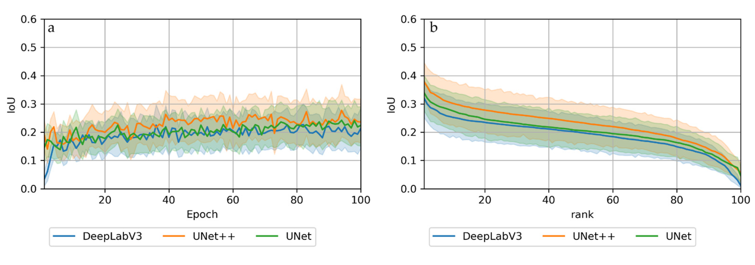
The applied AI segmentation models performed similarly, but with certain differences and slightly diverging performances. In all configurations, the training performance increased with increasing epochs (Figure 9a and Figure A10). Furthermore, the validation performance exceeded training metrics from the beginning, and typically plateaued from around 50 epochs. The good early validation performance compared to the training shows the effect of augmentation and indicates low overfitting.
3.1.2. Regional Comparison
The regionally stratified cross-validation on the sparse training sets highlighted the regional differences in thaw slumps across the Arctic with regard to environmental conditions, data quality and data availability. Overall, regional differences were more pronounced than model specifics or configurations, such as architecture and encoder. In the following, named regions indicate the validation (unseen) dataset, while the remaining regions were used for training (regionally stratified cross-validation).
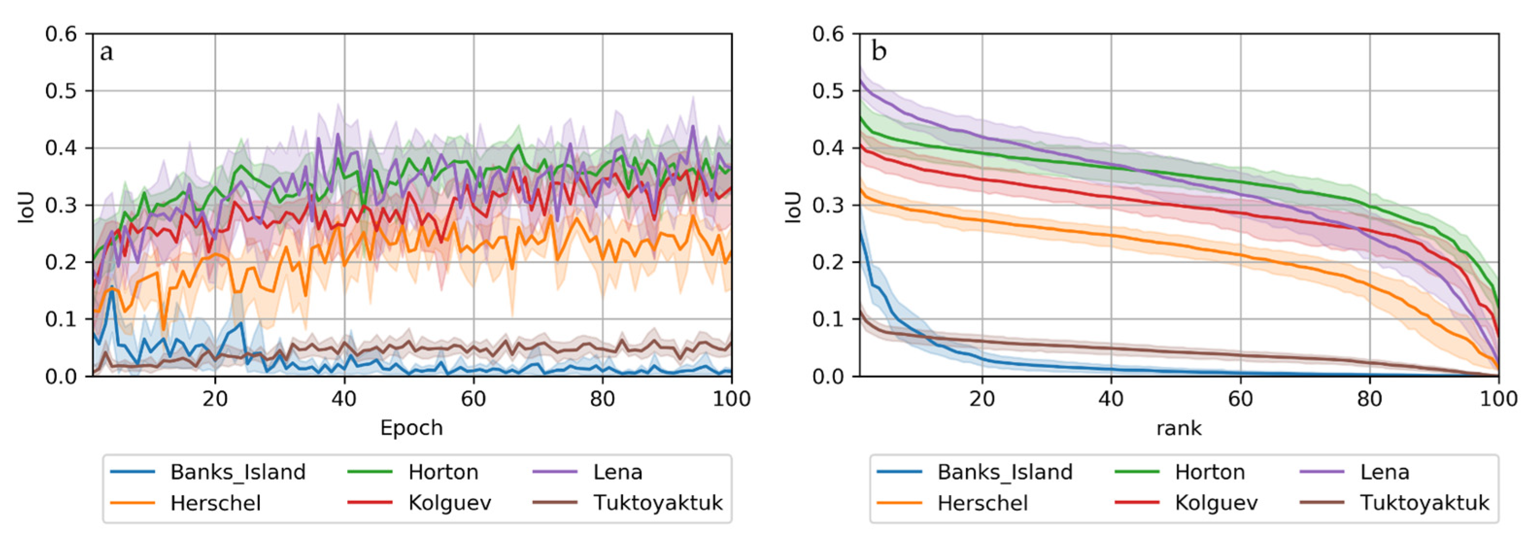
The Lena validation set achieved the best results (best model, see Table 5) with maximum IoU scores of 0.58 (UNet++ Resnet34), followed by Horton (0.55, UNet++ Resnet101), Kolguev (0.48, UNet++ Resnet101) and Herschel (0.38, DeepLabv3 Resnet34). Banks Island (UNet++ Resnet50) achieved a maximum IoU of 0.39, but this deteriorated quickly, seemingly due to strong overfitting. Tuktoyaktuk (UNet++ Resnet101) only achieved a maximum IoU of 0.15, with very little improvement even after several epochs (Figure 4a).
Although the best models per region performed similarly, the mean/ensemble performance of all models per region typically differed much more significantly (Figure 4). For many regions, individual models behaved differently in terms of volatility and learning success.
The maximum accuracies/scores of validation sets typically plateaued after around 40 epochs with almost all configurations (Figure 4a), except for Banks Island. Banks Island achieved individual IoU scores > 0.2 during early epochs, and these converged quickly towards zero during later epochs, which suggests insufficient spatial transferability likely due to overfitting. Tuktoyaktuk suffered from low scores throughout the entire training period, with only little variation in its IoU of around <0.1. The difference in segmentation performance between the best and next models was typically small, except for Banks Island, as shown in the sorted model performance illustrations (Figure 4b).
3.1.3. Model Configurations
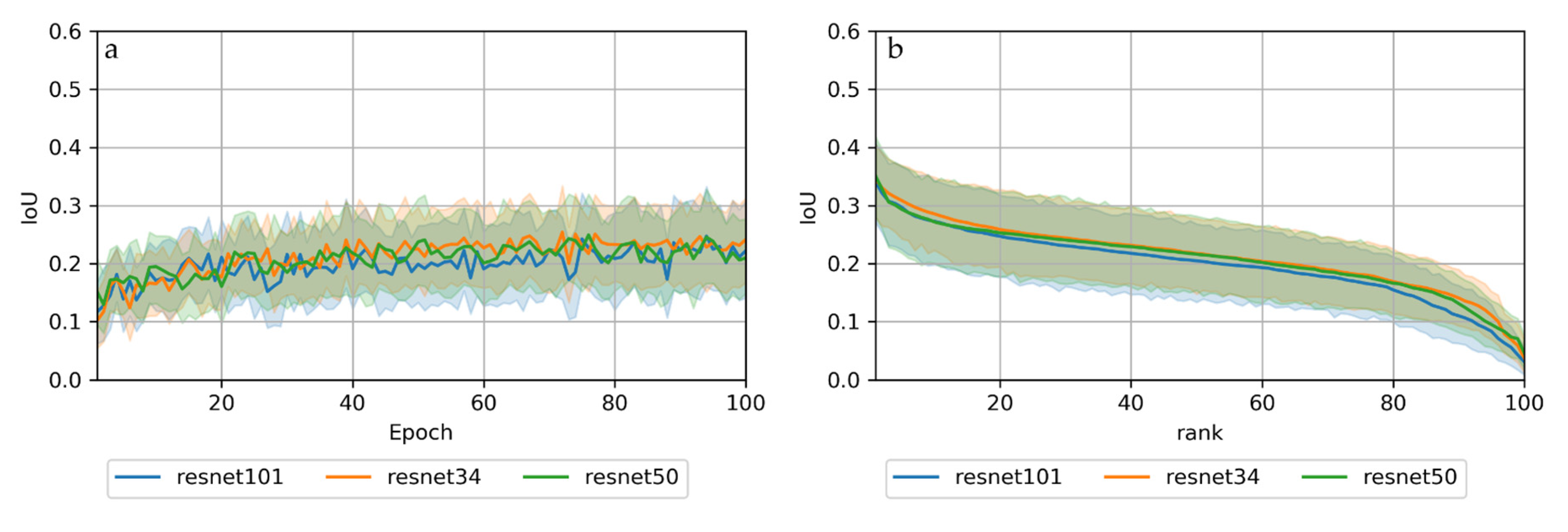
Among the tested configurations, including architectures and encoders, we only observed little differences in segmentation performance. However, overall, UNet++ outperformed UNet and DeepLabv3 consistently in this particular area (Figure 5). The choice of encoder only produced minor differences, but overall, simpler models (Resnet 34 > Resnet50 > Resnet101) resulted in slightly better IoU scores than more complex encoders (Resnet34: meanIoU = 0.33; Resnet50: meanIoU = 0.32; Resnet101: meanIoU = 0.31). In some individual cases, complex encoders (Resnet101) outperformed simpler encoders (e.g., Horton or Kolguev) (see Figure A10).
3.1.4. Computation Performance
In all configurations, UNet was the fastest model with the least hardware requirements. UNet++ was ~60% slower (factor 1.6) than UNet, while DeepLabv3 improved training times by a factor of ~2.3 compared to UNet. The hardware requirements for GPU memory were in line with those for processing times, with UNet requiring the least resources, followed by UNet++ and DeepLabv3.
3.2. Inference/Spatial Model Output
Regional Cross-Validation
(1a) Sparse models: The sparse trained models, using only image tiles with positive samples (RTS), produced results ranging from unsatisfactory to acceptable (see Figure 4), depending on region and model used. Figure 6, Figure 7 and Figure 8 (left column) show that the detection of thaw slumps produces mixed results, with strong variation depending on the input image. Decision boundaries are often fuzzy, with probability values (p-values) between 20 and 80% of being an RTS, as predicted by the model. Many non-slump areas, e.g., flat uplands or water bodies, were classified as thaw slumps in numerous instances, thus creating an abundance of false-positives in these settings.
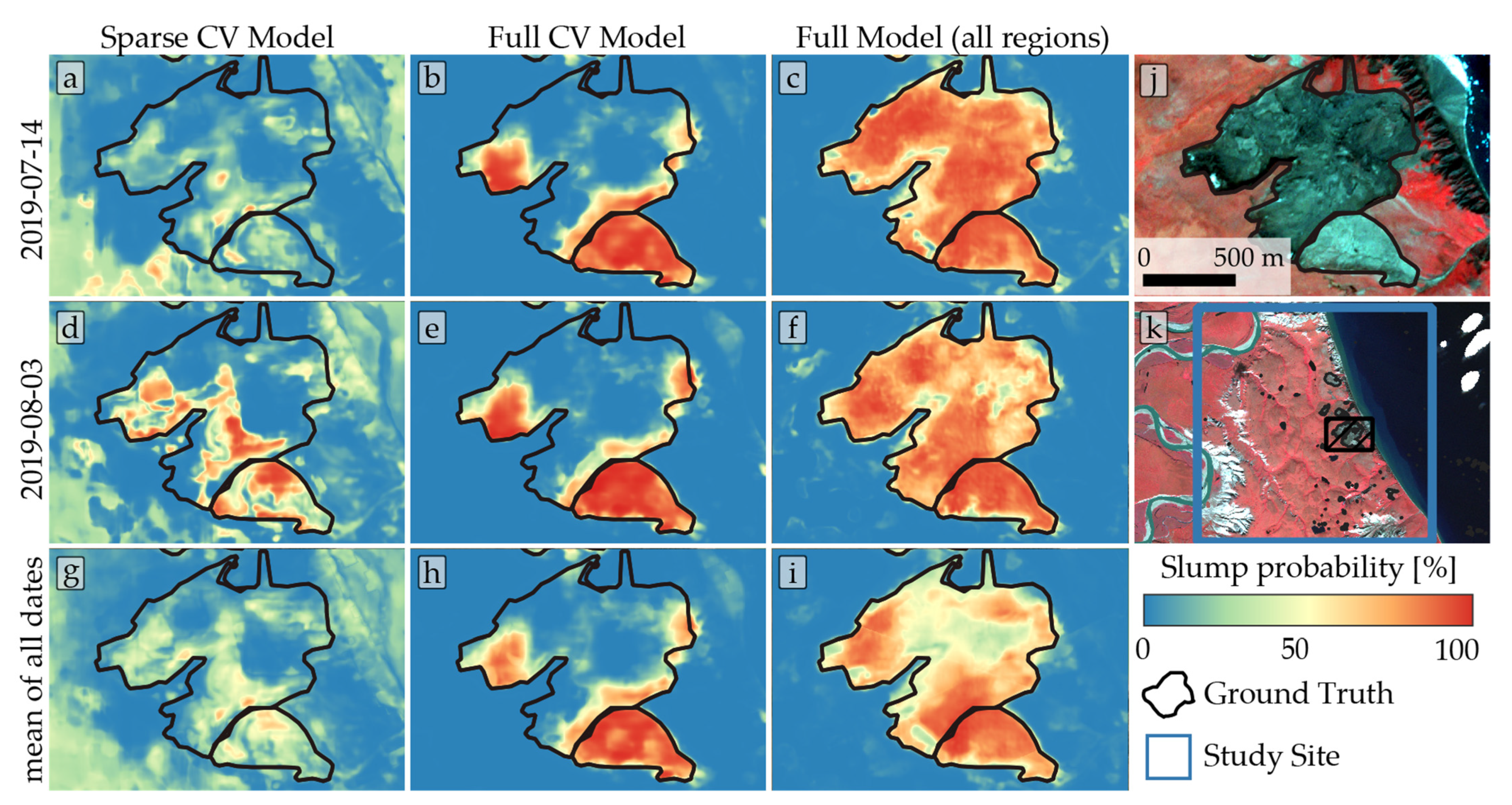
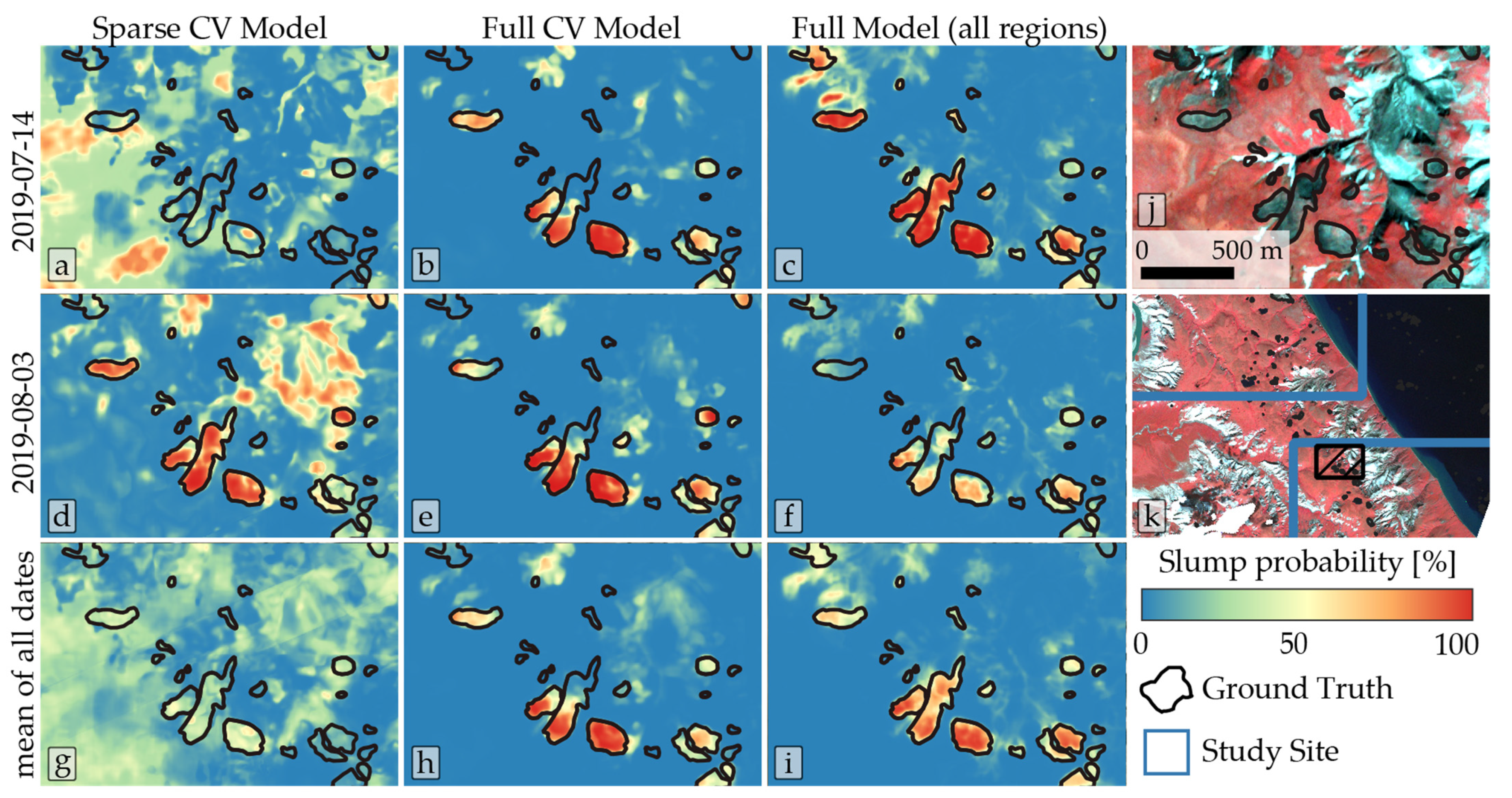
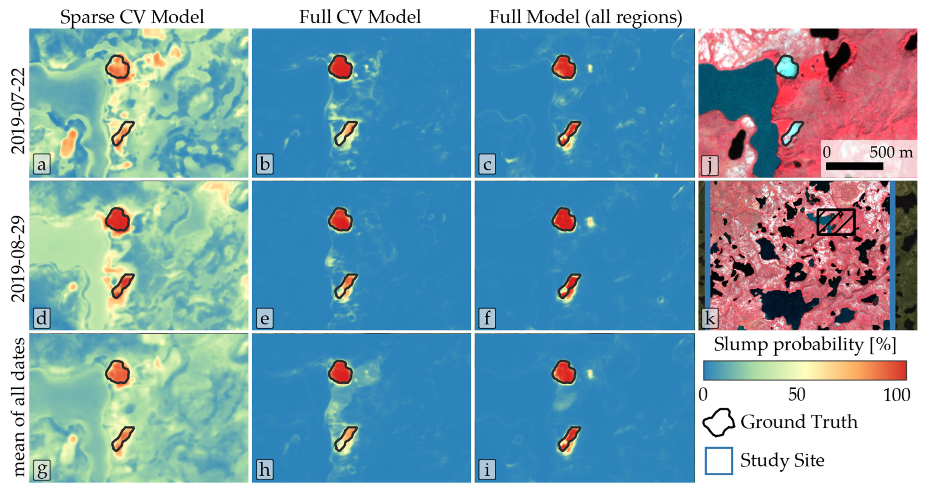
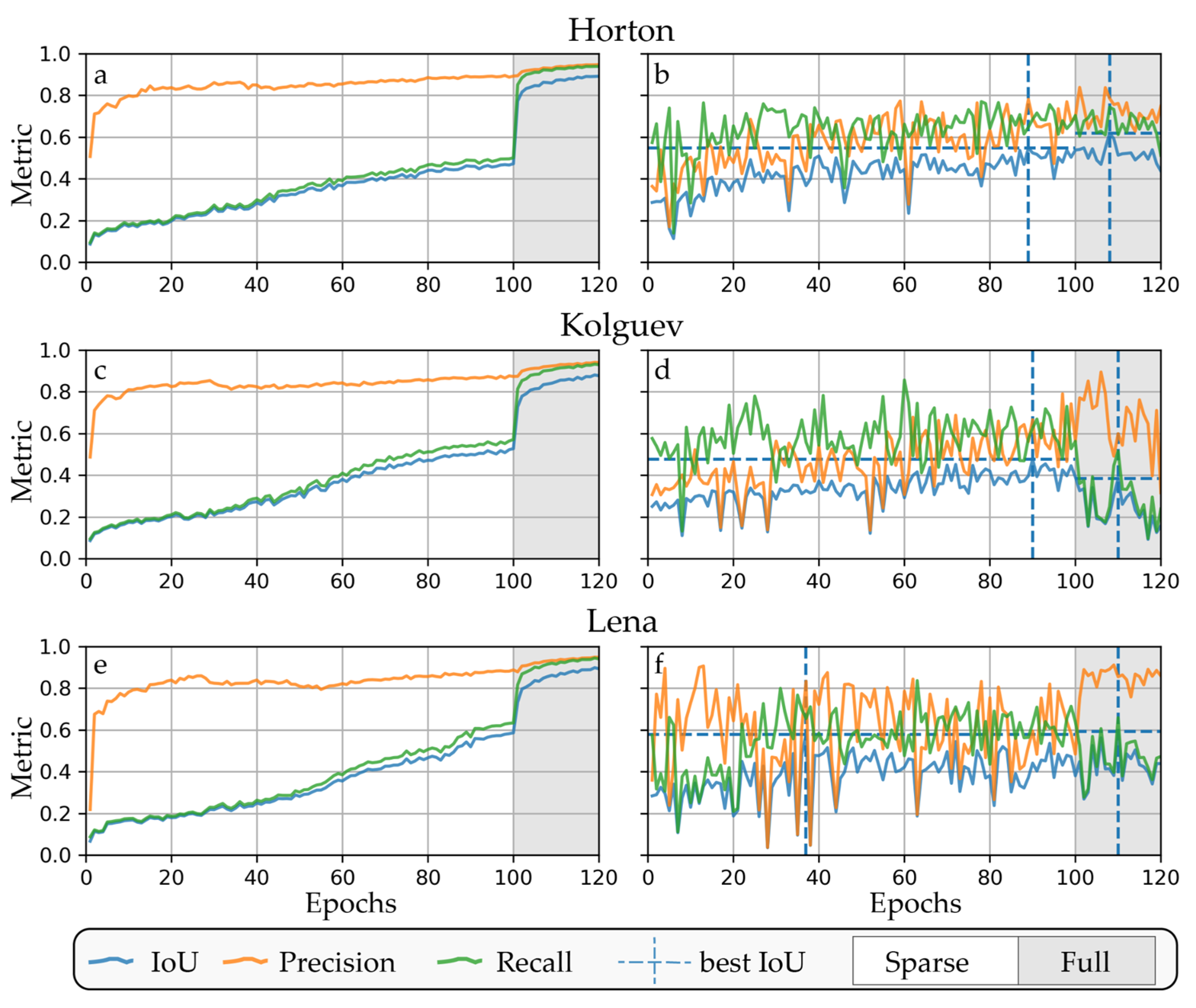
(1b) Fully trained models: After adding further training epochs with the entire dataset, using predominantly negative samples, the results were visually improved, with more distinct decision boundaries. This manifests in the improved precision but reduced recall (see Figure 9). However, the full accuracy metrics IoU and F1 increased (sparse/full; Horton Delta: IoU:0.62/ 0.55, F1: 0.76/0.71), stayed the same (Lena River: IoU:0.65/0.66, F1: 0.73/0.74) or even decreased (Kolguev Island: IoU:0.48/0.38, F1: 0.64/0.55) depending on the specific site.
Non-slump/disturbed areas were closer to 0% probability, while thaw slumps typically showed p-values close to 100%. The stability of classifications was significantly improved after the full training, as seen in Figure 6, Figure 7 and Figure 8, with comparable results between different dates (e.g., July and August).
However, misclassifications still occurred. False-positives occurred in rugged non-vegetated terrain (see Figure 6b,e,h and Figure 7b,e,h) or silty water bodies (see Figure 8b,e,h). As these false-positives are inconsistent between different images dates, taking into account multiple images dates can help to detect and minimize false-positive objects (see Figure 8 bottom row).
False-negatives are prevalent in many classified datasets. In most cases, parts of thaw slumps were not detected. As seen in Figure 6, Figure 7 and Figure 8, the slump area in proximity to the headwall was detected, whereas the distal parts remained undetected. This behavior suggests that the model is rather sensitive to the presence of headwall and thus steep slopes.
(2) The models trained on the full dataset, including the analyzed area, e.g., Horton (Figure 6c,f,i and Figure 7c,f,i) or Lena (Figure 8c,f,i), performed well. When the model was trained on these datasets, the performance was high, as expected. The model also classified well when used for periods (2020, 2021) outside of the training data period (2018, 2019). Furthermore, RTS just outside the specific 10 × 10 km training sites, which were unknown to the model, were successfully identified.
The models also detected features that we did not define as RTS, but which have a similar appearance in remote sensing imagery. These are, e.g., borderline cases, where the distinction of slumps vs. non-slumps was difficult during the digitization processes, or other vegetation-less land surface types appeared. This further highlights the difficulties of manual thaw slump annotation/classification.
4. Discussion
The presented methodology provides a highly automated and reproducible proof of concept for the application of the novel deep learning-based segmentation of retrogressive thaw slumps across Arctic permafrost regions.
The results are promising, showing good agreement for some regions, with IoU scores of 0.55 and 0.58 for the best configurations. However, the performances for some of the regions, e.g., Tuktoyaktuk or Banks Island, were unsatisfactory and likely prone to overfitting. The comparison of model performance here to other studies and methods is hardly possible due to the different input data and regions and the lack of standardized training datasets. Still, many studies depend on manual or at least semi-automated methods [18,21] for detecting and segmenting RTS. Only Huang et al. [51] used a very similar deep learning methodology in the Beiluhe Region on the Tibetan Plateau. They achieved cross-validated F-scores of ~0.85, higher than our analysis with F-scores of 0.25 to 0.73. However, Huang et al. applied cross-validation within a single comparably homogeneous region, in contrast to the regional cross-validation approach across strongly varying landscapes in our study. High training accuracies and visual inference tests suggest a good model performance at least in proximity to the trained regions.
We tested different architectures, including UNet++, UNet, and DeepLabv3. The different model architectures performed similarly, but UNet++ produced on average the best results compared to UNet and DepLabV3, as shown in the original UNet++ paper [80].
The choice of encoders influenced the results only slightly, but on average, simpler encoders (Resnet34 > Resnet50 > Resnet101) achieved slightly better performances, although the original paper achieved higher accuracies with the more complex version [75]. We hypothesize that a simpler network might be slightly more resilient to overfitting. With a higher quantity and variability of training data across an even broader spatial extent, more complex and deeper architectures may become more favorable for segmenting RTS. As the technology is constantly evolving, with new DL architectures, packages and hardware, there is the potential for much further improvement in the near future.
The large range in the model performance between study sites compared to the performance between different model parameters suggests that regional landscape differences are by far the most influential factor in the successful delineation of RTS across permafrost landscapes. This magnifies the pressing need for representative and large training/ground truth datasets for specific geospatial targets, such as RTS in this case. Such a database does not exist yet for permafrost-specific features, in contrast to general remote sensing-based targets such as PatternNet [81] or EuroSat [82], or the standard photography databases, such as ImageNet [83]. Sufficiently large and spatially extensive ground truth data are particularly hard to find. The ArcticNet database [84] is the first remote sensing image database with a spatial focus on the Arctic, but this is limited to wetlands. For RTS, most openly accessible high-resolution polygon datasets are available for NW Canada [17,57], Alaska [25] and China [51,85]. For other studies, only RTS centroid coordinates are often made available in public archives [16], or detailed data are not accessible. Therefore, we want to propose the creation of an openly accessible pan-Arctic database for RTS and other important permafrost landscape features for the training of future DL-based applications aimed at detecting permafrost features and landscape change due to thaw and erosion.
However, such a database requires consistent data quality and standard procedures. During our manual ground truth creation, we encountered severe difficulty in delineating RTS. While the headwall was often clearly visible, the lower part of RTS was often highly ambiguous and hardly discernible. This difficulty makes the creation of consistent datasets, across different spatial regions and teams, even more challenging, thus requiring standardized protocols and a common effort among researchers.
The workflow is openly available (see code) and highly automated, and the data processing approach is transferable and reusable. However, access to VHR input data is required, which are largely only commercially available and/or accessible under very restricted licensing rules at this stage. This is a major limitation in transferability and scalability at the moment. Recently, Planet data are becoming more and more accessible to large groups of researchers free of charge through government-funded research programs, which allows their broader application in Big Data AI test cases such as our study.
The requirement for sufficiently powered hardware is very important. However, with the increasing level of GPU processing capacities, either in institutional systems or even freely accessible cloud services (e.g., Google colab), barriers against using AI-based systems will become increasingly lower for geoscientific object detection purposes.
The presented methodology has the potential to be used on a much larger spatial scale. However, such scaling to large regions requires more training data across different regions and better access to Planet data. Alternatively, free data sources, such as Sentinel-2, might be used as alternatives, but are limited by their lower spatial resolution used for small- to medium-sized landscape features.
5. Conclusions
With our study, we have laid the foundation for using deep learning-based methods to detect and segment RTS across the Arctic. Using a highly automated workflow in conjunction with state-of-the art DL model architectures, we were able to create sufficiently good and transferable models for several regions, as proven by regional cross-validation. Regional models worked sufficiently well, but spatial transferability is still an issue for some regions. Additionally, the creation of training datasets proved to be highly challenging due to the difficulties in delineating RTS. For scaling DL-based segmentation models to the entire pan-Arctic region, we propose a common effort to create large and high-quality training datasets to train and benchmark RTS detection models. With rapidly growing hardware capabilities and expanding data availability, the automated mapping and segmentation of RTS and other permafrost-related landscape features may be realized soon in order to better understand and predict the impact of climate change in the permafrost region.
Supplementary Materials
The following are available online at https://www.mdpi.com/article/10.3390/rs13214294/s1, Table S1: PlanetScope image_ids used for ground truth collection as well as model training and validation.
Author Contributions
I.N. designed the study, carried out most experiments and led the manuscript writing. K.H. led the software development and wrote the methodology section. S.B. created the majority of training datasets. G.G. co-acquired project funding and was responsible for supervision. All authors participated in writing, reviewing and editing the manuscript. All authors have read and agreed to the published version of the manuscript.
Funding
This study was funded by the HGF AI-CORE project. Additional funding was provided by the ESA CCI+ Permafrost and NSF Permafrost Discovery Gateway projects (NSF Grants #2052107 and #1927872). The MWFK Brandenburg provided funding for high-performance computing infrastructure within the Potsdam Arctic Innovation Lab at AWI.
Data Availability Statement
The main processing code is available at https://github.com/initze/thaw-slump-segmentation. Training Polygons and additional processing code are available at https://github.com/initze/DL_RTS_Paper. Unfortunately we cannot make the commercial PlanetScope input data available.
Acknowledgments
We thank the AWI IT department and the DLR EOC IT department for supporting the IT infrastructure for the HGF AI CORE project. We thank the reviewers for their valuable comments, which helped to improve the quality of the manuscript.
Conflicts of Interest
The authors declare no conflict of interest. The funders had no role in the design of the study; in the collection, analyses, or interpretation of data; in the writing of the manuscript, or in the decision to publish the results.
Appendix A
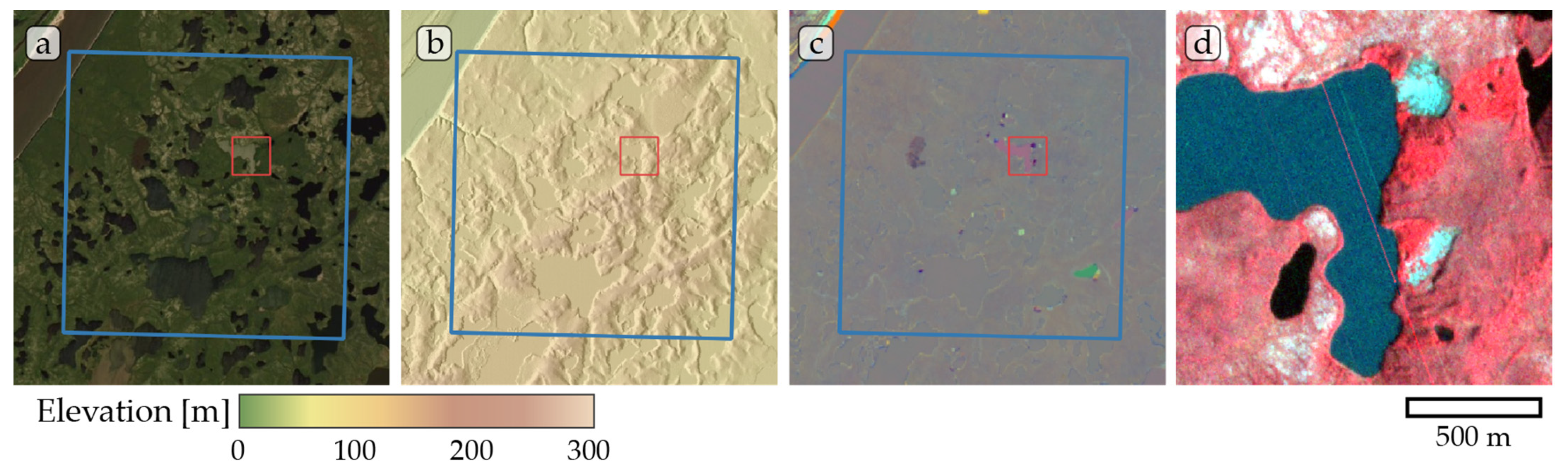
Figure A1.
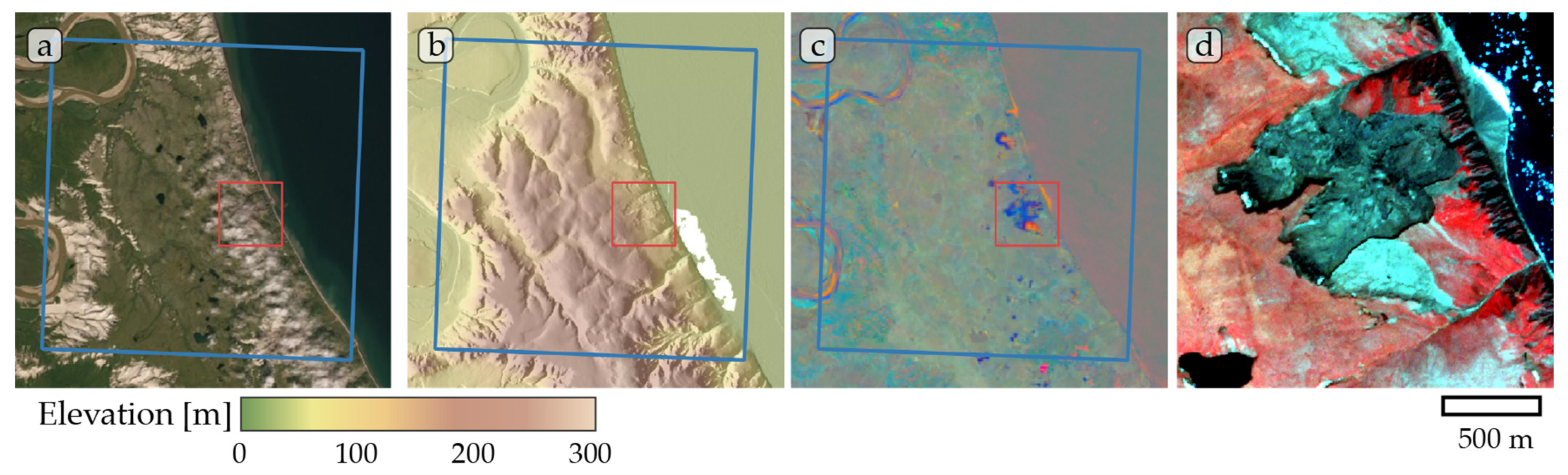
Study site Banks Island 01. (a) ESRI satellite layer, (b) ArcticDEM superimposed with hillshade, (c) Tasseled Cap trend visualization, (d) PlanetScope satellite image (NIR-R-G) acquired on 26 July 2019. Blue box, 10 × 10 km study site. Red box detailed view of (d).
Figure A1.
Study site Banks Island 01. (a) ESRI satellite layer, (b) ArcticDEM superimposed with hillshade, (c) Tasseled Cap trend visualization, (d) PlanetScope satellite image (NIR-R-G) acquired on 26 July 2019. Blue box, 10 × 10 km study site. Red box detailed view of (d).

Figure A2.
Study site Banks Island 02. (a) ESRI satellite layer, (b) ArcticDEM superimposed with hillshade, (c) Tasseled Cap trend visualization, (d) PlanetScope satellite image (NIR-R-G) acquired on 27 July 2019. Blue box, 10 × 10 km study site. Red box detailed view of (d).
Figure A2.
Study site Banks Island 02. (a) ESRI satellite layer, (b) ArcticDEM superimposed with hillshade, (c) Tasseled Cap trend visualization, (d) PlanetScope satellite image (NIR-R-G) acquired on 27 July 2019. Blue box, 10 × 10 km study site. Red box detailed view of (d).

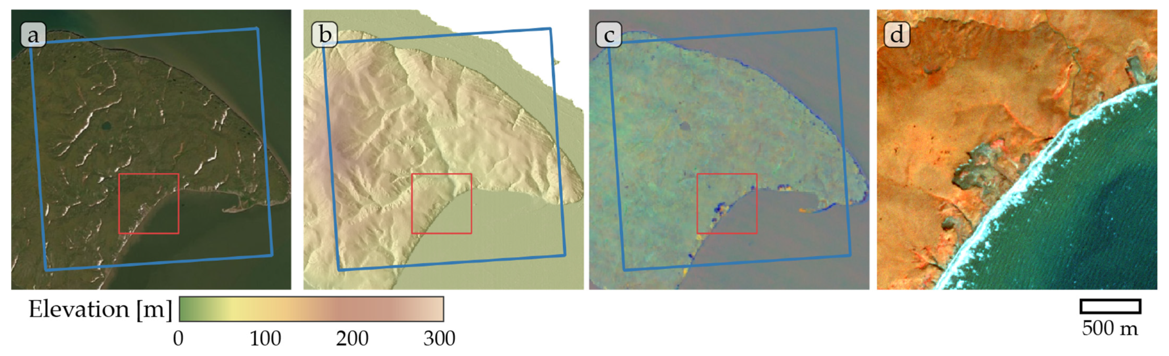
Figure A3.
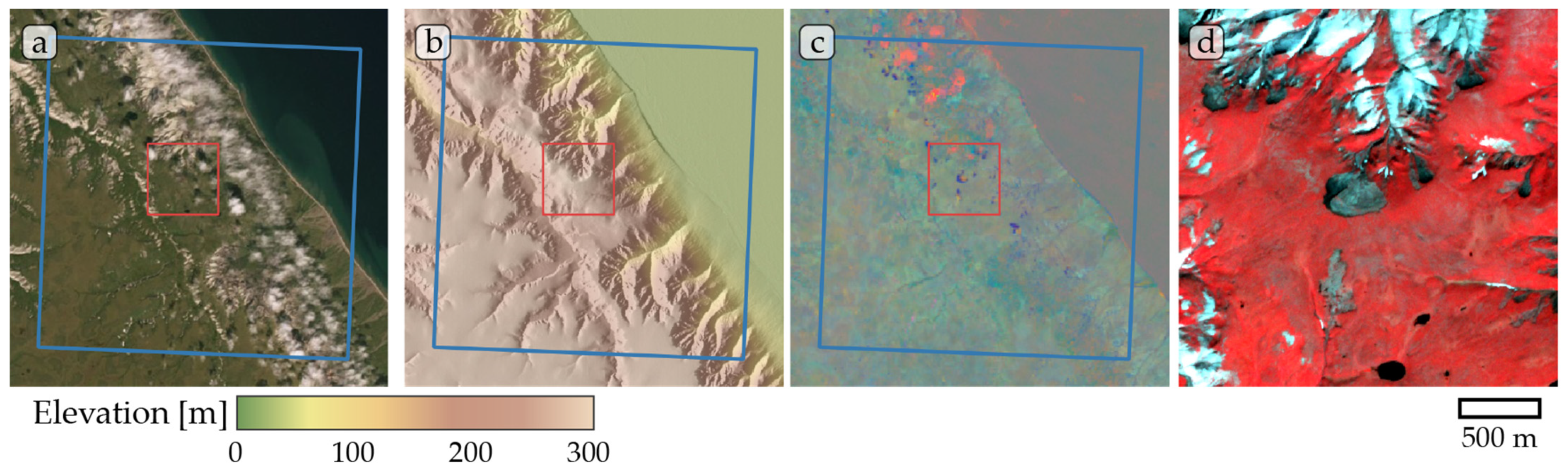
Study site Herschel Island 02. (a) ESRI satellite layer, (b) ArcticDEM superimposed with hillshade, (c) Tasseled Cap trend visualization, (d) PlanetScope satellite image (NIR-R-G) acquired on 02 September 2019. Blue box, 10 × 10 km study site. Red box detailed view of (d).
Figure A3.
Study site Herschel Island 02. (a) ESRI satellite layer, (b) ArcticDEM superimposed with hillshade, (c) Tasseled Cap trend visualization, (d) PlanetScope satellite image (NIR-R-G) acquired on 02 September 2019. Blue box, 10 × 10 km study site. Red box detailed view of (d).

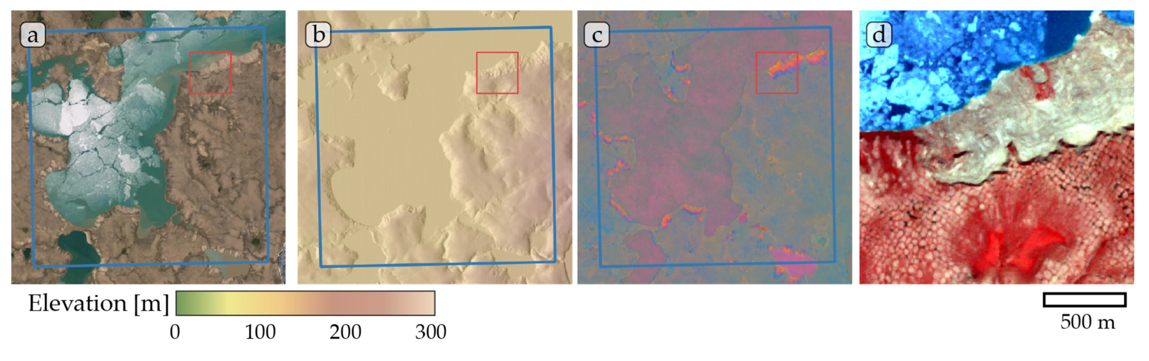
Figure A4.
Study site Horton 01. (a) ESRI satellite layer, (b) ArcticDEM superimposed with hillshade, (c) Tasseled Cap trend visualization, (d) PlanetScope satellite image (NIR-R-G) acquired on 14 July 2019. Blue box, 10 × 10 km study site. Red box detailed view of (d).
Figure A4.
Study site Horton 01. (a) ESRI satellite layer, (b) ArcticDEM superimposed with hillshade, (c) Tasseled Cap trend visualization, (d) PlanetScope satellite image (NIR-R-G) acquired on 14 July 2019. Blue box, 10 × 10 km study site. Red box detailed view of (d).

Figure A5.
Study site Horton 02. (a) ESRI satellite layer, (b) ArcticDEM superimposed with hillshade, (c) Tasseled Cap trend visualization, (d) PlanetScope satellite image (NIR-R-G) acquired on 27 July 2019. Blue box, 10 × 10 km study site. Red box detailed view of (d).
Figure A5.
Study site Horton 02. (a) ESRI satellite layer, (b) ArcticDEM superimposed with hillshade, (c) Tasseled Cap trend visualization, (d) PlanetScope satellite image (NIR-R-G) acquired on 27 July 2019. Blue box, 10 × 10 km study site. Red box detailed view of (d).

Figure A6.
Study site Kolguev Island 01. (a) ESRI satellite layer, (b) ArcticDEM superimposed with hillshade, (c) Tasseled Cap trend visualization, (d) PlanetScope satellite image (NIR-R-G) acquired on 22 August 2019. Blue box, 10 × 10 km study site. Red box detailed view of (d). Note partially missing ArcticDEM data in (b).

Figure A7.
Study site Kolguev Island 02. (a) ESRI satellite layer, (b) ArcticDEM superimposed with hillshade, (c) Tasseled Cap trend visualization, (d) PlanetScope satellite image (NIR-R-G) acquired on 19 August 2019. Blue box, 10 × 10 km study site. Red box detailed view of (d). Note partially missing ArcticDEM data in (b).

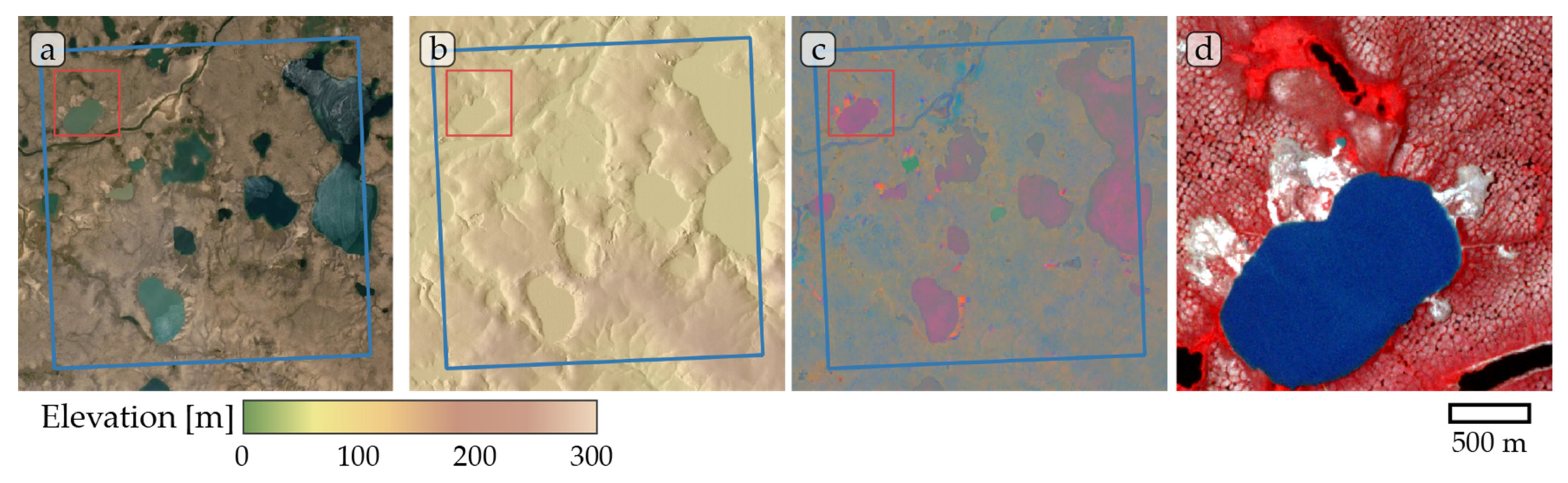
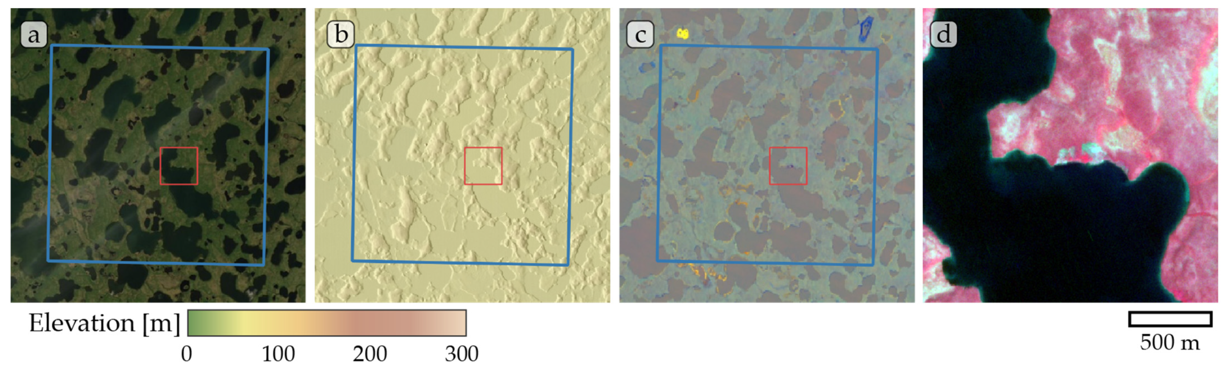
Figure A8.
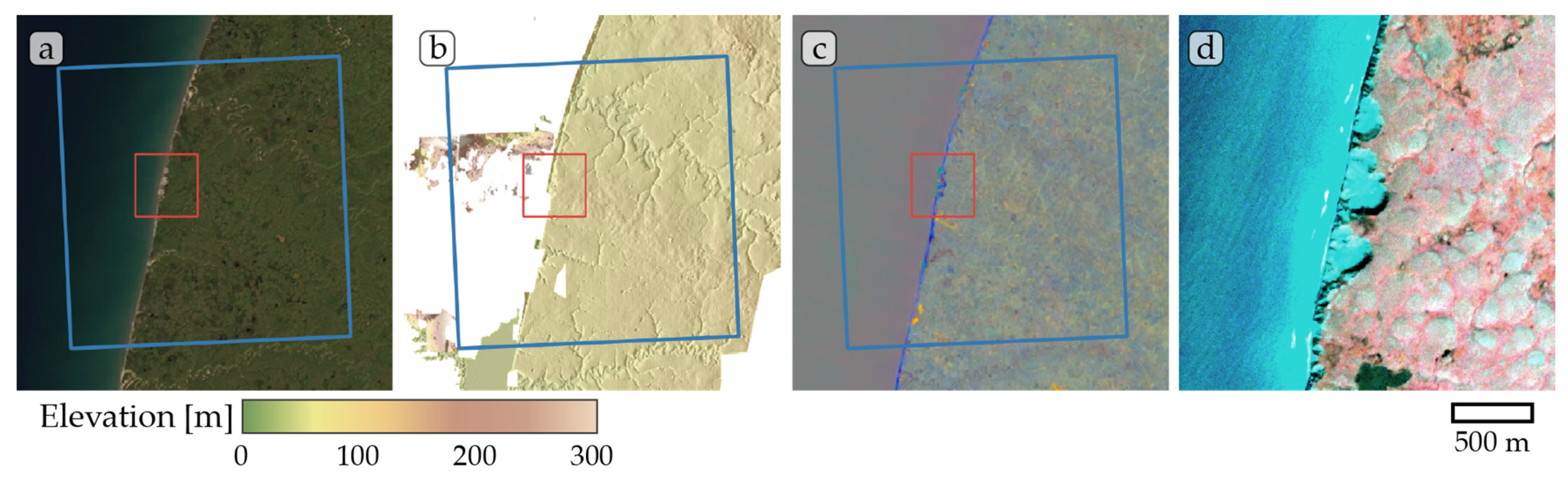
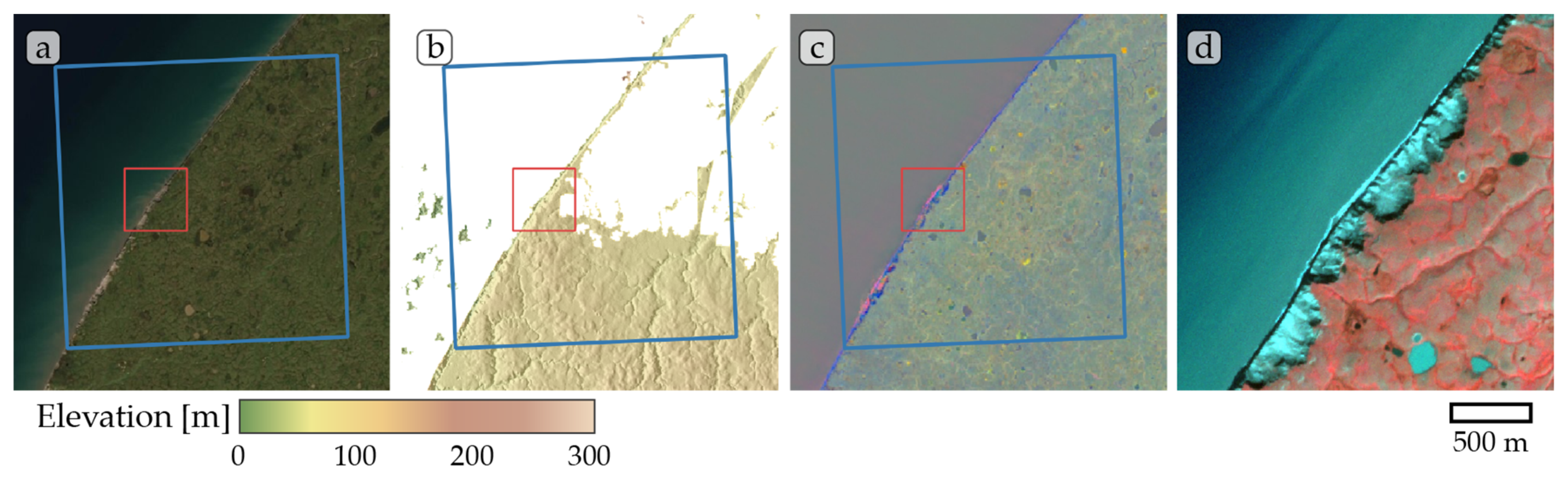
Study site Lena. (a) ESRI satellite layer, (b) ArcticDEM superimposed with hillshade, (c) Tasseled Cap trend visualization, (d) PlanetScope satellite image (NIR-R-G) acquired on 31 July 2019. Blue box, 10 × 10 km study site. Red box detailed view of (d).
Figure A8.
Study site Lena. (a) ESRI satellite layer, (b) ArcticDEM superimposed with hillshade, (c) Tasseled Cap trend visualization, (d) PlanetScope satellite image (NIR-R-G) acquired on 31 July 2019. Blue box, 10 × 10 km study site. Red box detailed view of (d).

Figure A9.
Study site Tuktoyaktuk. (a) ESRI satellite layer, (b) ArcticDEM superimposed with hillshade, (c) Tasseled Cap trend visualization, (d) PlanetScope satellite image (NIR-R-G) acquired on 13 July 2019. Blue box, 10 × 10 km study site. Red box detailed view of (d).
Figure A9.
Study site Tuktoyaktuk. (a) ESRI satellite layer, (b) ArcticDEM superimposed with hillshade, (c) Tasseled Cap trend visualization, (d) PlanetScope satellite image (NIR-R-G) acquired on 13 July 2019. Blue box, 10 × 10 km study site. Red box detailed view of (d).

Figure A10.
Mean and standard deviation of IoU scores per encoder sorted by (a) epoch and by (b) scores (best to worst). n = 18 (6 sites × 3 architectures) per encoder.
Figure A10.
Mean and standard deviation of IoU scores per encoder sorted by (a) epoch and by (b) scores (best to worst). n = 18 (6 sites × 3 architectures) per encoder.

References
- Box, J.E.; Colgan, W.T.; Christensen, T.R.; Schmidt, N.M.; Lund, M.; Parmentier, F.-J.W.; Brown, R.; Bhatt, U.S.; Euskirchen, E.S.; Romanovsky, V.E.; et al. Key Indicators of Arctic Climate Change: 1971–2017. Environ. Res. Lett. 2019, 14, 045010. [Google Scholar] [CrossRef]
- Meredith, M.; Sommerkorn, M.; Cassotta, S.; Derksen, C.; Ekaykin, A.; Hollowed, A.; Kofinas, G.; Mackintosh, A.; Melbourne-Thomas, J.; Muelbert, M.M.C. Polar Regions. Chapter 3, IPCC Special Report on the Ocean and Cryosphere in a Changing Climate; WMO: Geneva, Switzerland, 2019. [Google Scholar]
- Biskaborn, B.K.; Smith, S.L.; Noetzli, J.; Matthes, H.; Vieira, G.; Streletskiy, D.A.; Schoeneich, P.; Romanovsky, V.E.; Lewkowicz, A.G.; Abramov, A.; et al. Permafrost Is Warming at a Global Scale. Nat. Commun. 2019, 10, 264. [Google Scholar] [CrossRef] [Green Version]
- Nitzbon, J.; Westermann, S.; Langer, M.; Martin, L.C.P.; Strauss, J.; Laboor, S.; Boike, J. Fast Response of Cold Ice-Rich Permafrost in Northeast Siberia to a Warming Climate. Nat. Commun. 2020, 11, 2201. [Google Scholar] [CrossRef] [PubMed]
- Vasiliev, A.A.; Drozdov, D.S.; Gravis, A.G.; Malkova, G.V.; Nyland, K.E.; Streletskiy, D.A. Permafrost Degradation in the Western Russian Arctic. Environ. Res. Lett. 2020, 15, 045001. [Google Scholar] [CrossRef]
- Hugelius, G.; Strauss, J.; Zubrzycki, S.; Harden, J.W.; Schuur, E.A.G.; Ping, C.-L.; Schirrmeister, L.; Grosse, G.; Michaelson, G.J.; Koven, C.D.; et al. Estimated Stocks of Circumpolar Permafrost Carbon with Quantified Uncertainty Ranges and Identified Data Gaps. Biogeosciences 2014, 11, 6573–6593. [Google Scholar] [CrossRef] [Green Version]
- Strauss, J.; Schirrmeister, L.; Grosse, G.; Wetterich, S.; Ulrich, M.; Herzschuh, U.; Hubberten, H. The Deep Permafrost Carbon Pool of the Yedoma Region in Siberia and Alaska. Geophys. Res. Lett. 2013, 40, 6165–6170. [Google Scholar] [CrossRef] [PubMed] [Green Version]
- Schuur, E.A.G.; McGuire, A.D.; Schädel, C.; Grosse, G.; Harden, J.W.; Hayes, D.J.; Hugelius, G.; Koven, C.D.; Kuhry, P.; Lawrence, D.M.; et al. Climate Change and the Permafrost Carbon Feedback. Nature 2015, 520, 171–179. [Google Scholar] [CrossRef]
- Grosse, G.; Harden, J.; Turetsky, M.; McGuire, A.D.; Camill, P.; Tarnocai, C.; Frolking, S.; Schuur, E.A.G.; Jorgenson, T.; Marchenko, S.; et al. Vulnerability of High-Latitude Soil Organic Carbon in North America to Disturbance. J. Geophys. Res. Biogeosci. 2011, 116. [Google Scholar] [CrossRef] [Green Version]
- Burn, C.R.; Lewkowicz, A.G. CANADIAN LANDFORM EXAMPLES - 17 RETROGRESSIVE THAW SLUMPS. Can. Geogr. Géographe Can. 1990, 34, 273–276. [Google Scholar] [CrossRef]
- Lacelle, D.; Bjornson, J.; Lauriol, B. Climatic and Geomorphic Factors Affecting Contemporary (1950–2004) Activity of Retrogressive Thaw Slumps on the Aklavik Plateau, Richardson Mountains, NWT, Canada: Climatic and Geomorphic Factors Affecting Thaw Slump Activity. Permafr. Periglac. Process. 2010, 21, 1–15. [Google Scholar] [CrossRef]
- Lantuit, H.; Pollard, W.H. Fifty Years of Coastal Erosion and Retrogressive Thaw Slump Activity on Herschel Island, Southern Beaufort Sea, Yukon Territory, Canada. Geomorphology 2008, 95, 84–102. [Google Scholar] [CrossRef]
- Leibman, M.; Khomutov, A.; Kizyakov, A. Cryogenic Landslides in the West-Siberian Plain of Russia: Classification, Mechanisms, and Landforms. In Landslides in Cold Regions in the Context of Climate Change; Shan, W., Guo, Y., Wang, F., Marui, H., Strom, A., Eds.; Environmental Science and Engineering; Springer International Publishing: Cham, Germany, 2014; pp. 143–162. ISBN 978-3-319-00867-7. [Google Scholar]
- Ashastina, K.; Schirrmeister, L.; Fuchs, M.; Kienast, F. Palaeoclimate Characteristics in Interior Siberia of MIS 6–2: First Insights from the Batagay Permafrost Mega-Thaw Slump in the Yana Highlands. Clim. Past 2017, 13, 795–818. [Google Scholar] [CrossRef] [Green Version]
- Lantz, T.C.; Kokelj, S.V. Increasing Rates of Retrogressive Thaw Slump Activity in the Mackenzie Delta Region, N.W.T., Canada. Geophys. Res. Lett. 2008, 35, L06502. [Google Scholar] [CrossRef]
- Lewkowicz, A.G.; Way, R.G. Extremes of Summer Climate Trigger Thousands of Thermokarst Landslides in a High Arctic Environment. Nat. Commun. 2019, 10, 1329. [Google Scholar] [CrossRef] [PubMed] [Green Version]
- Segal, R.A.; Lantz, T.C.; Kokelj, S.V. Acceleration of Thaw Slump Activity in Glaciated Landscapes of the Western Canadian Arctic. Environ. Res. Lett. 2016, 11, 034025. [Google Scholar] [CrossRef]
- Ward Jones, M.K.; Pollard, W.H.; Jones, B.M. Rapid Initialization of Retrogressive Thaw Slumps in the Canadian High Arctic and Their Response to Climate and Terrain Factors. Environ. Res. Lett. 2019, 14, 055006. [Google Scholar] [CrossRef]
- Kokelj, S.V.; Lantz, T.C.; Kanigan, J.; Smith, S.L.; Coutts, R. Origin and Polycyclic Behaviour of Tundra Thaw Slumps, Mackenzie Delta Region, Northwest Territories, Canada. Permafr. Periglac. Process. 2009, 20, 173–184. [Google Scholar] [CrossRef]
- Balser, A.W.; Jones, J.B.; Gens, R. Timing of Retrogressive Thaw Slump Initiation in the Noatak Basin, Northwest Alaska, USA. J. Geophys. Res. Earth Surf. 2014, 119, 1106–1120. [Google Scholar] [CrossRef]
- Kokelj, S.V.; Lantz, T.C.; Tunnicliffe, J.; Segal, R.; Lacelle, D. Climate-Driven Thaw of Permafrost Preserved Glacial Landscapes, Northwestern Canada. Geology 2017, 45, 371–374. [Google Scholar] [CrossRef] [Green Version]
- Andreev, A.A.; Grosse, G.; Schirrmeister, L.; Kuznetsova, T.V.; Kuzmina, S.A.; Bobrov, A.A.; Tarasov, P.E.; Novenko, E.Y.; Meyer, H.; Derevyagin, A.Y.; et al. Weichselian and Holocene Palaeoenvironmental History of the Bol’shoy Lyakhovsky Island, New Siberian Archipelago, Arctic Siberia. Boreas 2009, 38, 72–110. [Google Scholar] [CrossRef] [Green Version]
- Lantuit, H.; Atkinson, D.; Paul Overduin, P.; Grigoriev, M.; Rachold, V.; Grosse, G.; Hubberten, H.-W. Coastal Erosion Dynamics on the Permafrost-Dominated Bykovsky Peninsula, North Siberia, 1951–2006. Polar Res. 2011, 30, 7341. [Google Scholar] [CrossRef]
- Kokelj, S.V.; Tunnicliffe, J.; Lacelle, D.; Lantz, T.C.; Chin, K.S.; Fraser, R. Increased Precipitation Drives Mega Slump Development and Destabilization of Ice-Rich Permafrost Terrain, Northwestern Canada. Glob. Planet. Chang. 2015, 129, 56–68. [Google Scholar] [CrossRef] [Green Version]
- Swanson, D.K. Permafrost Thaw-related Slope Failures in Alaska’s Arctic National Parks. 1980–2019. Permafr. Periglac. Process. 2021, 32, 392–406. [Google Scholar] [CrossRef]
- Babkina, E.A.; Leibman, M.O.; Dvornikov, Y.A.; Fakashchuk, N.Y.; Khairullin, R.R.; Khomutov, A.V. Activation of Cryogenic Processes in Central Yamal as a Result of Regional and Local Change in Climate and Thermal State of Permafrost. Russ. Meteorol. Hydrol. 2019, 44, 283–290. [Google Scholar] [CrossRef]
- Kizyakov, A.; Zimin, M.; Leibman, M.; Pravikova, N. Monitoring of the Rate of Thermal Denudation and Thermal Abrasion on the Western Coast of Kolguev Island, Using High Resolution Satellite Images. Kriosf. Zemli 2013, 17, 36–47. [Google Scholar]
- Vadakkedath, V.; Zawadzki, J.; Przeździecki, K. Multisensory Satellite Observations of the Expansion of the Batagaika Crater and Succession of Vegetation in Its Interior from 1991 to 2018. Environ. Earth Sci. 2020, 79, 150. [Google Scholar] [CrossRef] [Green Version]
- Obu, J.; Lantuit, H.; Grosse, G.; Günther, F.; Sachs, T.; Helm, V.; Fritz, M. Coastal Erosion and Mass Wasting along the Canadian Beaufort Sea Based on Annual Airborne LiDAR Elevation Data. Geomorphology 2017, 293, 331–346. [Google Scholar] [CrossRef] [Green Version]
- Swanson, D.; Nolan, M. Growth of Retrogressive Thaw Slumps in the Noatak Valley, Alaska, 2010–2016, Measured by Airborne Photogrammetry. Remote Sens. 2018, 10, 983. [Google Scholar] [CrossRef] [Green Version]
- van der Sluijs, J.; Kokelj, S.; Fraser, R.; Tunnicliffe, J.; Lacelle, D. Permafrost Terrain Dynamics and Infrastructure Impacts Revealed by UAV Photogrammetry and Thermal Imaging. Remote Sens. 2018, 10, 1734. [Google Scholar] [CrossRef] [Green Version]
- Nitze, I.; Grosse, G.; Jones, B.M.; Romanovsky, V.E.; Boike, J. Remote Sensing Quantifies Widespread Abundance of Permafrost Region Disturbances across the Arctic and Subarctic. Nat. Commun. 2018, 9, 5423. [Google Scholar] [CrossRef] [PubMed]
- Lara, M.J.; Chipman, M.L.; Hu, F.S. Automated Detection of Thermoerosion in Permafrost Ecosystems Using Temporally Dense Landsat Image Stacks. Remote Sens. Environ. 2019, 221, 462–473. [Google Scholar] [CrossRef]
- Runge, A.; Nitze, I.; Grosse, G. Remote Sensing Annual Dynamics of Rapid Permafrost Thaw Disturbances with LandTrendr. Remote Sens. Environ. accepted.
- Blaschke, T.; Lang, S.; Hay, G. Object-Based Image Analysis: Spatial Concepts for Knowledge-Driven Remote Sensing Applications; Springer Science & Business Media: Berlin/Heidelberg Germany, 2008. [Google Scholar]
- Zhu, X.X.; Tuia, D.; Mou, L.; Xia, G.-S.; Zhang, L.; Xu, F.; Fraundorfer, F. Deep Learning in Remote Sensing: A Comprehensive Review and List of Resources. IEEE Geosci. Remote Sens. Mag. 2017, 5, 8–36. [Google Scholar] [CrossRef] [Green Version]
- Ghorbanzadeh, O.; Blaschke, T.; Gholamnia, K.; Meena, S.; Tiede, D.; Aryal, J. Evaluation of Different Machine Learning Methods and Deep-Learning Convolutional Neural Networks for Landslide Detection. Remote Sens. 2019, 11, 196. [Google Scholar] [CrossRef] [Green Version]
- Prakash, N.; Manconi, A.; Loew, S. A New Strategy to Map Landslides with a Generalized Convolutional Neural Network. Sci. Rep. 2021, 11, 9722. [Google Scholar] [CrossRef] [PubMed]
- Wang, H.; Zhang, L.; Yin, K.; Luo, H.; Li, J. Landslide Identification Using Machine Learning. Geosci. Front. 2021, 12, 351–364. [Google Scholar] [CrossRef]
- Wagner, F.; Dalagnol, R.; Tarabalka, Y.; Segantine, T.; Thomé, R.; Hirye, M. U-Net-Id, an Instance Segmentation Model for Building Extraction from Satellite Images—Case Study in the Joanópolis City, Brazil. Remote Sens. 2020, 12, 1544. [Google Scholar] [CrossRef]
- Yang, N.; Tang, H. GeoBoost: An Incremental Deep Learning Approach toward Global Mapping of Buildings from VHR Remote Sensing Images. Remote Sens. 2020, 12, 1794. [Google Scholar] [CrossRef]
- Zhao, W.; Du, S.; Emery, W.J. Object-Based Convolutional Neural Network for High-Resolution Imagery Classification. IEEE J. Sel. Top. Appl. Earth Obs. Remote Sens. 2017, 10, 3386–3396. [Google Scholar] [CrossRef]
- Wagner, F.H.; Dalagnol, R.; Tagle Casapia, X.; Streher, A.S.; Phillips, O.L.; Gloor, E.; Aragão, L.E.O.C. Regional Mapping and Spatial Distribution Analysis of Canopy Palms in an Amazon Forest Using Deep Learning and VHR Images. Remote Sens. 2020, 12, 2225. [Google Scholar] [CrossRef]
- Abdalla, A.; Cen, H.; Abdel-Rahman, E.; Wan, L.; He, Y. Color Calibration of Proximal Sensing RGB Images of Oilseed Rape Canopy via Deep Learning Combined with K-Means Algorithm. Remote Sens. 2019, 11, 3001. [Google Scholar] [CrossRef] [Green Version]
- Bhuiyan, M.A.E.; Witharana, C.; Liljedahl, A.K.; Jones, B.M.; Daanen, R.; Epstein, H.E.; Kent, K.; Griffin, C.G.; Agnew, A. Understanding the Effects of Optimal Combination of Spectral Bands on Deep Learning Model Predictions: A Case Study Based on Permafrost Tundra Landform Mapping Using High Resolution Multispectral Satellite Imagery. J. Imaging 2020, 6, 97. [Google Scholar] [CrossRef] [PubMed]
- Park, J.H.; Inamori, T.; Hamaguchi, R.; Otsuki, K.; Kim, J.E.; Yamaoka, K. RGB Image Prioritization Using Convolutional Neural Network on a Microprocessor for Nanosatellites. Remote Sens. 2020, 12, 3941. [Google Scholar] [CrossRef]
- Abolt, C.J.; Young, M.H.; Atchley, A.L.; Wilson, C.J. Brief Communication: Rapid Machine-Learning-Based Extraction and Measurement of Ice Wedge Polygons in High-Resolution Digital Elevation Models. Cryosphere 2019, 13, 237–245. [Google Scholar] [CrossRef] [Green Version]
- Bhuiyan, M.A.E.; Witharana, C.; Liljedahl, A.K. Use of Very High Spatial Resolution Commercial Satellite Imagery and Deep Learning to Automatically Map Ice-Wedge Polygons across Tundra Vegetation Types. J. Imaging 2020, 6, 137. [Google Scholar] [CrossRef]
- Zhang, W.; Liljedahl, A.K.; Kanevskiy, M.; Epstein, H.E.; Jones, B.M.; Jorgenson, M.T.; Kent, K. Transferability of the Deep Learning Mask R-CNN Model for Automated Mapping of Ice-Wedge Polygons in High-Resolution Satellite and UAV Images. Remote Sens. 2020, 12, 1085. [Google Scholar] [CrossRef] [Green Version]
- Bartsch, A.; Pointner, G.; Ingeman-Nielsen, T.; Lu, W. Towards Circumpolar Mapping of Arctic Settlements and Infrastructure Based on Sentinel-1 and Sentinel-2. Remote Sens. 2020, 12, 2368. [Google Scholar] [CrossRef]
- Huang, L.; Luo, J.; Lin, Z.; Niu, F.; Liu, L. Using Deep Learning to Map Retrogressive Thaw Slumps in the Beiluhe Region (Tibetan Plateau) from CubeSat Images. Remote Sens. Environ. 2020, 237, 111534. [Google Scholar] [CrossRef]
- Huang, L.; Liu, L.; Luo, J.; Lin, Z.; Niu, F. Automatically Quantifying Evolution of Retrogressive Thaw Slumps in Beiluhe (Tibetan Plateau) from Multi-Temporal CubeSat Images. Int. J. Appl. Earth Obs. Geoinform. 2021, 102, 102399. [Google Scholar] [CrossRef]
- Lakeman, T.R.; England, J.H. Paleoglaciological Insights from the Age and Morphology of the Jesse Moraine Belt, Western Canadian Arctic. Quat. Sci. Rev. 2012, 47, 82–100. [Google Scholar] [CrossRef]
- Fraser, R.; Kokelj, S.; Lantz, T.; McFarlane-Winchester, M.; Olthof, I.; Lacelle, D. Climate Sensitivity of High Arctic Permafrost Terrain Demonstrated by Widespread Ice-Wedge Thermokarst on Banks Island. Remote Sens. 2018, 10, 954. [Google Scholar] [CrossRef] [Green Version]
- Walker, D.A.; Raynolds, M.K.; Daniëls, F.J.A.; Einarsson, E.; Elvebakk, A.; Gould, W.A.; Katenin, A.E.; Kholod, S.S.; Markon, C.J.; Melnikov, E.S.; et al. The Circumpolar Arctic Vegetation Map. J. Veg. Sci. 2005, 16, 267–282. [Google Scholar] [CrossRef]
- Obu, J.; Westermann, S.; Kääb, A.; Bartsch, A. Ground Temperature Map, 2000-2016, Northern Hemisphere Permafrost in Earth & Environmental Science; PANGAEA, 2018. [Google Scholar] [CrossRef]
- Ramage, J.L.; Irrgang, A.M.; Herzschuh, U.; Morgenstern, A.; Couture, N.; Lantuit, H. Terrain Controls on the Occurrence of Coastal Retrogressive Thaw Slumps along the Yukon Coast, Canada: Coastal RTSs Along the Yukon Coast. J. Geophys. Res. Earth Surf. 2017, 122, 1619–1634. [Google Scholar] [CrossRef]
- Fritz, M.; Wetterich, S.; Meyer, H.; Schirrmeister, L.; Lantuit, H.; Pollard, W.H. Origin and Characteristics of Massive Ground Ice on Herschel Island (Western Canadian Arctic) as Revealed by Stable Water Isotope and Hydrochemical Signatures: Origin and Characteristics of Massive Ground Ice on Herschel Island. Permafr. Periglac. Process. 2011, 22, 26–38. [Google Scholar] [CrossRef] [Green Version]
- Stauch, G.; Lehmkuhl, F. Quaternary Glaciations in the Verkhoyansk Mountains, Northeast Siberia. Quat. Res. 2010, 74, 145–155. [Google Scholar] [CrossRef]
- Burn, C.R.; Kokelj, S.V. The Environment and Permafrost of the Mackenzie Delta Area. Permafr. Periglac. Process. 2009, 20, 83–105. [Google Scholar] [CrossRef]
- Olthof, I.; Fraser, R.H.; Schmitt, C. Landsat-Based Mapping of Thermokarst Lake Dynamics on the Tuktoyaktuk Coastal Plain, Northwest Territories, Canada since 1985. Remote Sens. Environ. 2015, 168, 194–204. [Google Scholar] [CrossRef]
- Plug, L.J.; Walls, C.; Scott, B.M. Tundra Lake Changes from 1978 to 2001 on the Tuktoyaktuk Peninsula, Western Canadian Arctic. Geophys. Res. Lett. 2008, 35, L03502. [Google Scholar] [CrossRef]
- Planet Team. Planet Application Program Interface: In Space for Life on Earth. Planet. 2017. Available online: https://api.planet.com (accessed on 16 July 2021).
- Porter, C.; Morin, P.; Howat, I.; Noh, M.-J.; Bates, B.; Peterman, K.; Keesey, S.; Schlenk, M.; Gardiner, J.; Tomko, K.; et al. ArcticDEM [Data set]; Harvard Dataverse, 2018. [Google Scholar] [CrossRef]
- Li, J.; Roy, D. A Global Analysis of Sentinel-2A, Sentinel-2B and Landsat-8 Data Revisit Intervals and Implications for Terrestrial Monitoring. Remote Sens. 2017, 9, 902. [Google Scholar] [CrossRef] [Green Version]
- Roy, S.; Swetnam, T.L. Tyson-Swetnam/Porder: Porder: Simple CLI for Planet OrdersV2 API; Zenodo, 2020. [Google Scholar]
- Nitze, I.; Grosse, G.; Jones, B.; Arp, C.; Ulrich, M.; Fedorov, A.; Veremeeva, A. Landsat-Based Trend Analysis of Lake Dynamics across Northern Permafrost Regions. Remote Sens. 2017, 9, 640. [Google Scholar] [CrossRef] [Green Version]
- Nitze, I.; Grosse, G. Detection of Landscape Dynamics in the Arctic Lena Delta with Temporally Dense Landsat Time-Series Stacks. Remote Sens. Environ. 2016, 181, 27–41. [Google Scholar] [CrossRef]
- Huang, C.; Wylie, B.; Yang, L.; Homer, C.; Zylstra, G. Derivation of a Tasselled Cap Transformation Based on Landsat 7 At-Satellite Reflectance. Int. J. Remote Sens. 2002, 23, 1741–1748. [Google Scholar] [CrossRef]
- QGIS Development Team. QGIS Geographic Information System; QGIS Association, 2021. [Google Scholar]
- Nextgis/Quickmapservices. 2021. [Python]. NextGIS. (Original Work Published 2014). Available online: https://github.com/nextgis/quickmapservices (accessed on 7 July 2021).
- Segal, R.; Kokelj, S.; Lantz, T.; Durkee, K.; Gervais, S.; Mahon, E.; Snijders, M.; Buysse, J.; Schwarz, S. Broad-Scale Mapping of Terrain Impacted by Retrogressive Thaw Slumping in Northwestern Canada. NWT Open Rep. 2016, 8, 1–17. [Google Scholar]
- Paszke, A.; Gross, S.; Massa, F.; Lerer, A.; Bradbury, J.; Chanan, G.; Killeen, T.; Lin, Z.; Gimelshein, N.; Antiga, L.; et al. PyTorch: An Imperative Style, High-Performance Deep Learning Library. ArXiv191201703 Cs Stat 2019. [Google Scholar]
- Buslaev, A.; Iglovikov, V.I.; Khvedchenya, E.; Parinov, A.; Druzhinin, M.; Kalinin, A.A. Albumentations: Fast and Flexible Image Augmentations. Information 2020, 11, 125. [Google Scholar] [CrossRef] [Green Version]
- He, K.; Zhang, X.; Ren, S.; Sun, J. Deep Residual Learning for Image Recognition. In Proceedings of the 2016 IEEE Conference on Computer Vision and Pattern Recognition (CVPR), Las Vegas, NV, USA, 27–30 June 2016; pp. 770–778. [Google Scholar]
- Ronneberger, O. U-Net: Convolutional Networks for Biomedical Image Segmentation. In Proceedings of the International Conference on Medical Image Computing and Computer-Assisted Intervention; Springer: Cham, Germany, 2015; pp. 234–241. [Google Scholar]
- Zhou, Z.; Rahman Siddiquee, M.M.; Tajbakhsh, N.; Liang, J. UNet++: A Nested U-Net Architecture for Medical Image Segmentation. In Deep Learning in Medical Image Analysis and Multimodal Learning for Clinical Decision Support; Stoyanov, D., Taylor, Z., Carneiro, G., Syeda-Mahmood, T., Martel, A., Maier-Hein, L., Tavares, J.M.R.S., Bradley, A., Papa, J.P., Belagiannis, V., et al., Eds.; Lecture Notes in Computer Science; Springer International Publishing: Cham, Germany, 2018; Volume 11045, pp. 3–11. ISBN 978-3-030-00888-8. [Google Scholar]
- Chen, L.-C.; Papandreou, G.; Schroff, F.; Adam, H. Rethinking Atrous Convolution for Semantic Image Segmentation. ArXiv170605587 Cs 2017. [Google Scholar]
- Kingma, D.P.; Ba, J. Adam: A Method for Stochastic Optimization. ArXiv14126980 Cs 2017. [Google Scholar]
- Zhou, Z.; Siddiquee, M.M.R.; Tajbakhsh, N.; Liang, J. UNet++: Redesigning Skip Connections to Exploit Multiscale Features in Image Segmentation. IEEE Trans. Med. Imaging 2020, 39, 1856–1867. [Google Scholar] [CrossRef] [Green Version]
- Zhou, W.; Newsam, S.; Li, C.; Shao, Z. PatternNet: A Benchmark Dataset for Performance Evaluation of Remote Sensing Image Retrieval. ISPRS J. Photogramm. Remote Sens. 2018, 145, 197–209. [Google Scholar] [CrossRef] [Green Version]
- Helber, P.; Bischke, B.; Dengel, A.; Borth, D. EuroSAT: A Novel Dataset and Deep Learning Benchmark for Land Use and Land Cover Classification. IEEE J. Sel. Top. Appl. Earth Obs. Remote Sens. 2019, 12, 2217–2226. [Google Scholar] [CrossRef] [Green Version]
- Deng, J.; Dong, W.; Socher, R.; Li, L.-J.; Li, K.; Fei-Fei, L. ImageNet: A Large-Scale Hierarchical Image Database. In Proceedings of the 2009 IEEE Conference on Computer Vision and Pattern Recognition, Miami, FL, USA, 20–25 June 2009; pp. 248–255. [Google Scholar]
- Jiang, Z.; Von Ness, K.; Loisel, J.; Wang, Z. ArcticNet: A Deep Learning Solution to Classify the Arctic Area. In Proceedings of the Proceedings of the IEEE/CVF Conference on Computer Vision and Pattern Recognition Workshops, Long Beach, CA, USA, 16–17 June 2019; pp. 38–47. [Google Scholar]
- Xia, Z.; Huang, L.; Liu, L. An Inventory of Retrogressive Thaw Slumps Along the Vulnerable Qinghai-Tibet Engineering Corridor. 2021. Available online: https://doi.pangaea.de/10.1594/PANGAEA.933957 (accessed on 19 October 2021).
Figure 1.
Overview map of study sites and permafrost extent based on (Obu et al., 2018).

Figure 2.
Temporal distribution of input data by study region.

Figure 3.
Flowchart of the full processing pipeline.

Figure 4.
Mean and standard deviation of IoU scores per site sorted by (a) epoch and (b) scores (best to worst). n = 9 (3 sites × 3 encoders) per region.
Figure 4.
Mean and standard deviation of IoU scores per site sorted by (a) epoch and (b) scores (best to worst). n = 9 (3 sites × 3 encoders) per region.

Figure 5.
Mean and standard deviation of IoU scores per architecture sorted by (a) epoch and (b) scores (best to worst). n = 18 (6 sites × 3 encoders) per architecture.
Figure 5.
Mean and standard deviation of IoU scores per architecture sorted by (a) epoch and (b) scores (best to worst). n = 18 (6 sites × 3 encoders) per architecture.

Figure 6.
Detection results in subset of Horton Delta 01 study site with the modeled RTS probability on two different image dates ((a–c): 14 July 2019; (d–f): 03 August 2019) and the mean of all dates (g–i) as well as three different models ((a,d,g): sparse cross-validation model; (b,e,h): full cross-validation model; (c,f,i): full model trained on all regions). The subset of a multispectral false-color PlanetScope image (NIR-R-G) with ground truth is shown in panel (j). Panel (k) shows the approximate location of the subset within the study region.

Figure 7.
Detection results in the subset of the Horton Delta 02 study site with the modeled RTS probability on two different image dates ((a–c): 14 July 2019; (d–f): 03 August 2019) and the mean of all dates (g–i) as well as three different models ((a,d,g): sparse cross-validation model; (b,e,h): full cross-validation model; (c,f,i): full model trained on all regions). The subset of a multispectral false-color PlanetScope image (NIR-R-G) with ground truth is shown in panel (j). Panel (k) shows the approximate location of the subset within the study region.

Figure 8.
Detection results in the subset of the Lena River study site with the modeled RTS probability on two different image dates ((a–c): 22 July 2019; (d–f): 29 August 2019) and the mean of all dates (g–i) as well as three different models ((a,d,g): sparse cross-validation model; (b,e,h): full cross-validation model; (c,f,i): full model trained on all regions). The subset of a multispectral false-color PlanetScope image (NIR-R-G) with ground truth is shown in panel (j). Panel (k) shows the approximate location of the subset within the study region.

Figure 9.
Training (a,c,e) and validation (b,d,f) metrics of best models for the three best regions with sparse and full training.
Figure 9.
Training (a,c,e) and validation (b,d,f) metrics of best models for the three best regions with sparse and full training.


Table 1.
Study sites with center coordinates, region, and number of used Planet images.
| Study Site | Center Coordinates | Region | # of Images | # of Image Dates |
|---|---|---|---|---|
| Banks Island 01 | 119.50° W; 72.84° N; | NW Canada | 12 | 5 |
| Banks Island 02 | 118.20° W; 73.04° N | NW Canada | 15 | 4 |
| Herschel Island | 139.00° W; 69.60° N | NW Canada | 10 | 5 |
| Horton Delta 01 | 126.75° W; 69.75° N; | NW Canada | 10 | 4 |
| Horton Delta 02 | 126.60° W; 69.64° N | NW Canada | 13 | 6 |
| Kolguev Island 01 | 48.35° E; 69.22° N | NW Siberia | 29 | 14 |
| Kolguev Island 02 | 48.51° E; 69.35° N | NW Siberia | 20 | 8 |
| Lena River | 124.40° E; 69.12° N | E Siberia | 47 | 22 |
| Tuktoyaktuk Pen. | 133.80° W; 69.12° N | NW Canada | 19 | 9 |
Table 2.
Study sites with total number of detected RTS and number of individual RTS per date.
| Study Site | # of Total Individual RTS Objects | # of Individual RTS per Date 1, 2 | Median Object Size (m²) |
|---|---|---|---|
| Banks Island 01 | 397 | 65–103 | 22,032 |
| Banks Island 02 | 151 | 24–53 | 22,203 |
| Herschel Island | 148 | 15–40 | 5175 |
| Horton Delta 01 | 180 | 36–52 | 5562 |
| Horton Delta 02 | 354 | 35–67 | 7981 |
| Kolguev Island 01 | 44 | 3–5 | 78,786 |
| Kolguev Island 02 | 275 | 25–41 | 13,840 |
| Lena River | 238 | 5–13 | 14,470 |
| Tuktoyaktuk Pen. | 385 | 30–55 | 2229 |
1 Total image size may be different between dates, e.g., incomplete coverage. 2 PlanetScope data have some image overlap, which may lead to (partially) duplicated vectors.
Table 3.
List of model input data layers, with preprocessing status, native resolution and number of bands.
Table 3.
List of model input data layers, with preprocessing status, native resolution and number of bands.
| Input Data | Raw/Derived | Native Resolution (m) | # Bands |
|---|---|---|---|
| PlanetScope Scene (SR) | Raw | 3 | 3 |
| PlanetScope NDVI | Derived | 3 | 1 |
| ArcticDEM relative elevation | Derived | 2 | 1 |
| ArcticDEM slope | Derived | 2 | 1 |
| TCVIS | Derived | 30 | 3 |
Table 4.
List of model inference output data layers.
| Output Data | Format | Resolution (m) |
|---|---|---|
| Polygon vector | ESRI Shapefile | - |
| Binary raster | GTiff | 3 |
| Probability raster | GTiff | 3 |
Table 5.
Regional performance of best sparse models. U++: UNet++; DLv3: DeepLabv3; Rn34: Resnet34; Rn50: Resnet50; Rn101: Resnet101. IoU1/Prec1/Recall1/F11: Metrics of best sparse regional CV model. IoU5: 5th best model of 100. IoU10: 10th best model of 100.
Table 5.
Regional performance of best sparse models. U++: UNet++; DLv3: DeepLabv3; Rn34: Resnet34; Rn50: Resnet50; Rn101: Resnet101. IoU1/Prec1/Recall1/F11: Metrics of best sparse regional CV model. IoU5: 5th best model of 100. IoU10: 10th best model of 100.
| Study Site | Model Config. | IoU1 | IoU5 | IoU10 | Prec1 | Recall1 | F11 |
|---|---|---|---|---|---|---|---|
| Banks Island | U++Rn50 | 0.39 | 0.13 | 0.08 | 0.80 | 0.38 | 0.52 |
| Herschel | DLv3Rn34 | 0.39 | 0.33 | 0.32 | 0.50 | 0.63 | 0.56 |
| Horton | U++Rn101 | 0.55 | 0.54 | 0.51 | 0.78 | 0.77 | 0.71 |
| Kolguev | U++Rn101 | 0.48 | 0.45 | 0.43 | 0.67 | 0.63 | 0.64 |
| Lena | U++Rn34 | 0.58 | 0.51 | 0.50 | 0.83 | 0.65 | 0.73 |
| Tuktoyaktuk | U++Rn50 | 0.15 | 0.09 | 0.08 | 0.42 | 0.18 | 0.25 |
Publisher’s Note: MDPI stays neutral with regard to jurisdictional claims in published maps and institutional affiliations. |
© 2021 by the authors. Licensee MDPI, Basel, Switzerland. This article is an open access article distributed under the terms and conditions of the Creative Commons Attribution (CC BY) license (https://creativecommons.org/licenses/by/4.0/).
Share and Cite
MDPI and ACS Style
Nitze, I.; Heidler, K.; Barth, S.; Grosse, G. Developing and Testing a Deep Learning Approach for Mapping Retrogressive Thaw Slumps. Remote Sens. 2021, 13, 4294. https://doi.org/10.3390/rs13214294
AMA Style
Nitze I, Heidler K, Barth S, Grosse G. Developing and Testing a Deep Learning Approach for Mapping Retrogressive Thaw Slumps. Remote Sensing. 2021; 13(21):4294. https://doi.org/10.3390/rs13214294
Chicago/Turabian StyleNitze, Ingmar, Konrad Heidler, Sophia Barth, and Guido Grosse. 2021. "Developing and Testing a Deep Learning Approach for Mapping Retrogressive Thaw Slumps" Remote Sensing 13, no. 21: 4294. https://doi.org/10.3390/rs13214294
Note that from the first issue of 2016, this journal uses article numbers instead of page numbers. See further details here.