Technical Note

Monitoring the Transformation of Arctic Landscapes: Automated Shoreline Change Detection of Lakes Using Very High Resolution Imagery

1
Permafrost Research Section, Alfred Wegener Institute Helmholtz Centre for Polar and Marine Research, Telegrafenberg A45, 14473 Potsdam, Germany
2
Geography Department, Humboldt-Universität zu Berlin, Unter den Linden 6, 10099 Berlin, Germany
3
Institute of Geosciences, University of Potsdam, Karl-Liebknecht-Str. 24-25, 14476 Potsdam, Germany
*
Author to whom correspondence should be addressed.
Remote Sens. 2021, 13(14), 2802; https://doi.org/10.3390/rs13142802
Submission received: 7 June 2021 / Revised: 30 June 2021 / Accepted: 14 July 2021 / Published: 16 July 2021
(This article belongs to the Special Issue Dynamic Disturbance Processes in Permafrost Regions)

Abstract

:
Water bodies are a highly abundant feature of Arctic permafrost ecosystems and strongly influence their hydrology, ecology and biogeochemical cycling. While very high resolution satellite images enable detailed mapping of these water bodies, the increasing availability and abundance of this imagery calls for fast, reliable and automatized monitoring. This technical work presents a largely automated and scalable workflow that removes image noise, detects water bodies, removes potential misclassifications from infrastructural features, derives lake shoreline geometries and retrieves their movement rate and direction on the basis of ortho-ready very high resolution satellite imagery from Arctic permafrost lowlands. We applied this workflow to typical Arctic lake areas on the Alaska North Slope and achieved a successful and fast detection of water bodies. We derived representative values for shoreline movement rates ranging from 0.40–0.56 m yr−1 for lake sizes of 0.10 ha–23.04 ha. The approach also gives an insight into seasonal water level changes. Based on an extensive quantification of error sources, we discuss how the results of the automated workflow can be further enhanced by incorporating additional information on weather conditions and image metadata and by improving the input database. The workflow is suitable for the seasonal to annual monitoring of lake changes on a sub-meter scale in the study areas in northern Alaska and can readily be scaled for application across larger regions within certain accuracy limitations.

Graphical Abstract

1. Introduction

Arctic and Boreal permafrost lowlands are featured by a high abundance of water bodies [1,2,3,4], which have been important and very dynamic landscape components of these regions since the end of the Last Ice Age [5]. Apart from wetlands, (abandoned) river streams and relict lakes from the Pleistocene, in ice-rich permafrost regions, we often find water bodies that develop as a consequence of thermokarst processes [3] where soil subsidence triggered by the melting of excess ground ice leads to the formation and expansion of a pond [4,6]. Water influx from precipitation and runoff in the catchment adding to the ponding can alter the thermal regime of the ground in these poorly drained lowland regions with often poorly developed runoff systems [4,7] and further amplify the permafrost thaw. Regardless of their origin, Arctic water bodies play a major role in the geomorphological, hydrological, ecological and biogeochemical dynamics of permafrost landscapes [8,9,10,11]. It is therefore critically important to understand their changes under a warming climate and the resulting consequences of these changes. A central challenge in the efficient monitoring of current lake changes and the projection of their future developments is their often small size (down to only a few meters in diameter [2,7,12]), their vast abundance in lowland landscapes and their rapid (sometimes non-gradual) changes including formation, expansion and drainage.
Numerous studies have investigated lake changes in the Arctic using the analysis of multi-temporal imagery at different spatial resolutions and scales. While studies using low to medium resolution imagery such as Landsat (30 m spatial resolution) or MODIS (250 m) have allowed for the detection of water bodies larger than 1–10 ha [13,14], respectively, across large regions [15,16], they were limited in terms of the spatial detail of shoreline movement changes. In contrast, very high resolution (better than 1 m) airborne (UAV, planes) and satellite imagery allows for a detailed quantification of these changes. However, due to the lack of automated workflows, their analysis has been limited to small study areas and a limited number of analyzed lakes so far [12,17,18,19]. Existing research on shoreline movement rates of water bodies is generally based on the time-intensive manual digitization of the shorelines along a low number of selected shore transects on decadal time scales, which results in temporally highly averaged movement rates (e.g., [12]). These averages could mask the temporal and spatial variations of changes in Arctic water bodies and potential links to environmental drivers that can occur over shorter time periods of only a few years [20,21].
With the increasing availability of multi-temporal very high resolution imagery for large regions, even in the remote Arctic, highly automated workflows for lake shoreline analysis would facilitate detailed insights into the rapid thermo-hydrological dynamics of these landscapes in a changing climate.
Several studies have automatized individual steps for lake change mapping: (i) Shah et al. (2011) [22] established a method for extracting shorelines from Landsat imagery on a sub-pixel scale with an accuracy matching the quality of very high resolution data from sensors such as Quickbird, etc.; (ii) Sheng et al. (2008) [23] developed an automated image registration procedure on the basis of lake centroids; (iii) Bangira et al. (2019) [24] tested dynamic thresholding approaches such as the Otsu algorithm [25] to map water bodies with different characteristics in turbidity, sedimentation and eutrophication; (iv) Tian et al. (2017) [26] proposed a shoreline derivation approach by applying a non local active contour model on imagery classified with the Normalized Difference Water Index (NDWI) and (v) Cooley et al. (2017; 2019) [27,28] and Nitze et al. (2017) [29] used the automated processing of Cubesat imagery with object tracking to create high temporal change maps of lake extent and drainage in Arctic–Boreal regions of Alaska. These mapping approaches, however, did not target the automatized extraction of specific shoreline movement rates over time.
The objective of our study was to design a largely automated workflow that quantifies lake shoreline changes by deriving their shoreline geometry, movement rate and direction from satellite imagery with very high resolutions better than 1 m. Requirements for the workflow were (i) to be independent of the image scale, spatial resolution and water body geometry, (ii) to calculate rates of lake shoreline movements over seasonal to annual time periods and (iii) to derive shoreline movement directions.

2. Materials and Methods

We chose Python as a free and open-source processing tool so that the workflow can be easily adapted to user needs. Python provides the necessary speed for code execution, an open source environment, options for automation with existing libraries and the scaling of the processing environment. Figure 1 illustrates the processing pipeline. While the pan-sharpening and co-registration of the imagery are part of the manual pre-processing, the automated workflow (marked by the dashed lines) consists of the following processing steps: image noise removal, water body detection, filtering for water body sizes and elimination of misclassification originating from infrastructure elements and the calculation of shoreline movement rates and directions. We used manual quality assessment in order to evaluate the automated workflow.

2.1. Study Areas and Data

We analyzed two study sites that feature lakes that vary in size and geometry in the North American Arctic. They are located along the Dalton Highway in the North Slope Borough of Alaska, about 10 km (Deadhorse) and 40 km (mile post (MP) 396) inland from the Beaufort Sea (Figure 2A). Both sites belong to the continuous permafrost region [30] and are characterized by a cold Arctic climate with a mean annual air temperature of −11.4 °C, ranging from −27.6 °C in February to 7.6 °C in July (1981–2010 climate normals at Deadhorse station) [31]. The sites display a typical tundra vegetation of sedges, grasses and dwarf-shrub to moss-rich wetlands [32].
The study site around Deadhorse (Figure 2B), as part of the eastern Arctic Coastal Plain, is characterized by numerous thermokarst lakes and ponds with a circular to elliptical shape [8,18,33,34]. It covers 34 km2. The site at MP 396 further south was selected to evaluate the performance of the water body detection under different landscape conditions. It covers 23 km2 and is characterized by fewer water bodies—mainly oxbow lakes of the Sagavanirktok River with an elliptical to almost linear geometry (see Figure 2C). Both sites are underlain by ice-rich permafrost with ice wedge polygons [35].
At the Deadhorse study site, we used multi-temporal very high resolution imagery from the Quickbird-2 and WorldView-2/3 satellite sensors, covering the period from 2006 to 2016, with acquisitions every 3 to 4 years. For the analysis at site MP 396, one satellite image from 2016 was available. The imagery provides resolutions of 0.3 m to 0.7 m in the panchromatic band and 2.0 m to 2.8 m in the near-infrared (NIR) and visible (RGB) bands (Table 1).
Multi-spectral bands were pan-sharpened and resampled to a joint resolution of 0.5 m using the arcpy library. Images were then spatially co-registered with the automatic image-to-image registration tool in Environment for Visual Images Software (ENVI 5.5) before entering the subsequent workflow.
The images contained infrastructural elements such as roads, pipelines, buildings and oil exploration pads. Some of these features produced shadows which are often incorrectly identified as water. To filter out potentially misclassified features and to exclude artificial water basins next to exploration pads, we acquired the latest OpenStreetMap (OSM) [36] dataset for Alaska from 30 August 2019. Shapefiles containing information on industrial landuse, buildings and transportation routes were selected.

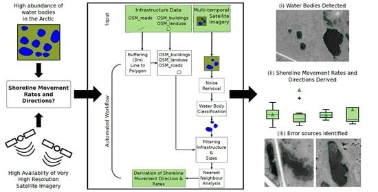
2.2. Automated Shoreline Change Detection Workflow

The shoreline change detection workflow consisted of four automated steps: (i) image noise removal, (ii) water body detection and shoreline geometry vectorization, (iii) the elimination of potential misclassifications from infrastructural elements and (iv) the derivation of shoreline movement rates and directions (see Figure 1).

2.2.1. Noise Removal

Some images showed speckle from sunglint over the water bodies related to the view angle, weather and wave conditions [37,38]. The speckle was highest in the RGB bands and decreased in the NIR band. Due to the pan-sharpening, the speckle-affected pixels were transferred to the NIR band, which was used afterwards for the water body detection. A median filter was applied using the scikit-image Python library [39] in order to reduce the image noise while preserving the edges for the shoreline derivation. A small filter radius removed noise that was only 1–2 pixels wide. In contrast, the speckle over our target water bodies often consisted of at least 30 relatively brighter pixels in a wave-like pattern. Therefore, filter radii ranging from 1 to 20 pixels at an interval of 2 pixels were tested on an image subset. A median radius of 5 pixels resulted in a homogeneous water surface without speckle but sharp shorelines. Values larger than 5 pixels did not enhance the result any further.

2.2.2. Water Body Detection

After the noise removal, a simple single band thresholding was performed on the pan-sharpened NIR band in order to distinguish water from non-water surfaces. Water bodies only exhibit the reflectance of shortwave radiation ( λ < 600 nm ); longwave radiation (from λ > 800 nm ), in contrast, is typically completely absorbed by the water body [40]. This electromagnetic characteristic clearly distinguished water bodies from the surrounding land surface in the imagery. The grey-scale value histograms of the near-infrared bands at the study site complied with this bi-modality, showing two peaks: one for an 8-bit grey-scale value of 0 (representing the satellite image margin) followed by values ranging between 25 and 80 (representing water bodies) on the one side and another major peak at value 255, representing sediments of the Sagavanirktok river and infrastructure surfaces. These appeared to be almost white on the satellite image due to their (gravel) consistency. Images were classified using Otsu thresholding [25]. The Otsu algorithm performed an adaptive segmentation of bi-modal imagery. It automatically derived a threshold value between the two peaks and classified the image accordingly. The classification resulted in a binary raster file extracting water bodies which was then converted into a vector file for the subsequent analysis.

2.2.3. Removal of Misclassifications and Infrastructural Elements

Subsequently, the workflow used infrastructure data from the OSM files in order to remove misclassified non-water body objects associated with infrastructure and infrastructure shadows. All linear infrastructure objects, such as roads, were polygonized by applying a 3 m-buffer and were merged with the remaining OSM files to generate a homogeneous MultiPolygon file. The OSM file and the classification result (delineated in orange in Figure 3A,B) were overlaid, and every polygon classified as a water body that intersected with an infrastructural element from the OSM dataset was excluded. Further, we filtered out all water bodies smaller than 0.1 ha. This minimum value was chosen to maintain consistency when referring to former baseline studies, which were mainly based on the analysis of Landsat imagery. Jones et al. [12] defined a minimum value of 0.1 ha since it approximately described the size of a pond in the center of a low-center polygon. As a result, the final classification file contained all water bodies over 0.1 ha as multipolygons (delineated in green in Figure 3A,B), excluding artificial water basins and shadows cast by infrastructural elements.

2.2.4. Calculation of Movement Rates

Following the classification and subsequent vectorization, all lake shorelines were represented by irregularly-sized line segments and vertices. In the workflow, changes in shoreline position were evaluated by calculating distances between neighboring polygon vertices from different dates. In order to enhance the spatial resolution for shoreline comparison, the number of vertices was increased along the segment lines of the polygons, with vertices every 0.5 m, complying with the spatial resolution of the input images. The shoreline segments were then converted to points. A nearest-points analysis was used to correlate each shoreline vertex from one date to the nearest vertex of the following date (Figure 3C). Subsequently, the distance and angle between the correlated vertices were calculated and saved as an attribute value for each point of the dataset. This procedure was repeated for every time step in the image stack. For the consecutive quality assessment, a net shoreline movement rate for every lake was derived, averaging over all points of the dataset.

2.3. Quality Assessment

We conducted a visual examination [41] of the detected lake shorelines to assess the workflow quality. Since this examination procedure relied on the same raw data, it strictly delivered only a quality assessment of the shoreline detection procedure without further ground truthing. We sub-sampled a total of 100 lakes from all time steps in the Deadhorse study site according to the data distribution: (i) strong outliers with very high or very low values in water surface area changes and shoreline movement rates, (ii) lakes within the minimum (25%-percentile − 1.5∗interquartile range) and maximum value (75%-percentile + 1.5∗interquartile range) of the data and (iii) outliers close to the minimum and maximum value. In a first step, we looked at the derived shoreline geometry of the water body. The decision of a correct identification was made if the following criteria were satisfied: the shoreline geometry needed to be captured fully, with all its complexities—e.g., polygonal collapse, connecting troughs leading to adjacent lakes etc. Only minor inaccuracies (such as vegetation covering part of the shoreline) at one position were accepted. Furthermore, we disregarded gaps in the lake center (e.g., occurring from sunglint etc.) since this study focused on the shoreline movement rate and direction, not the changes in water surface area. Once a water body was deemed correct, we evaluated the subsequent time step. If the lake shoreline was again accurately derived, the calculated movement rate was considered correct. Any sources for a false derivation were identified and recorded. Moreover, the detected water bodies were categorized according to their sizes, corresponding to exponentially scaled size categories used in previous Landsat-based lake studies [16,18], where a water surface pixel was 30 × 30 m :
  • 0.1–0.36 ha
  • 0.36–1.44 ha
  • 1.44–5.76 ha
  • 5.76–23.04 ha
  • >23.04 ha
Ultimately, a median annual shoreline movement rate and mean direction (averaged over the acquisition span of 3 and 4 years, respectively) was derived for every size category from the lakes that lay within the range of correctly flagged values.
In the case of the MP 396 study site, where only one time step was analyzed to evaluate the workflow performance on the extraordinary shape of oxbow lakes, a sub-sample was not needed. Further, only the accuracy of the derived shoreline was assessed, not the movement.

3. Results

3.1. Evaluation of the Workflow

3.1.1. Code and Performance

The Python script was run on a Linux Ubuntu server (system version 16.04.6 LTS) with a 64-bit architecture with 12 CPUs and a memory of 23 GB. The noise filtering and Otsu algorithm application with the subsequent vectorization of the water bodies for every image (with a size of 1.6 GB, covering the study site extent) took about 95 min. The calculation of the shoreline movement rate and direction was completed after an additional 25 min.

3.1.2. Quality of Noise Removal

Whereas the imagery in the years from 2006 to 2013 only needed little to no filtering, the 2016 image displayed high speckle from sunglint. In both cases, the median filter successfully removed the image noise while sharp borders of the water bodies were largely preserved. The filter was most efficient in the centre of the lakes where it produced a smooth water surface. In the shoreline area, the derivation was often inaccurate and was found to be related to sediment input from the shores or a shallow lake depth with a visible lake bottom. Further details can be found in Section 3.1.6.

3.1.3. Accuracy of Water Body Detection and Filtering

The Otsu thresholding provided a clear derivation of the shoreline, also capturing complex geometries; e.g., polygonal collapse into a lake and the existence of drainage channels or gullies. Even smaller ponding of water along roads and water-filled troughs within the polygonal-patterned ground were detected (see orange patches in Figure 3A). Shadows cast from buildings were misinterpreted as water bodies due to their similar spectral signature. However, these misclassifications were thoroughly removed when we filtered out the infrastructural elements with the OSM dataset.
A total of 665 lakes in four image time steps were identified in the 34 km2 Deadhorse study area and 66 lakes in the 23 km2 MP 396 study area for the year 2016. They were larger than 0.1 ha and not associated with infrastructural elements.
Of the resulting 665 LakeID files for the Deadhorse study site, 195 were empty, indicating that this particular lake could not be detected in the subsequent time step, and therefore no shoreline movement rate and direction could be calculated. Table 2 shows the number of detected lakes, empty files and lakes for which the shoreline movement rate and direction was calculated, broken down into the five lake size categories. In total, 71 to 83% of the detected water bodies were smaller than 1.44 ha, making small lakes and ponds the dominant landform. At both study sites, only few lakes larger than 5.76 ha were observed.

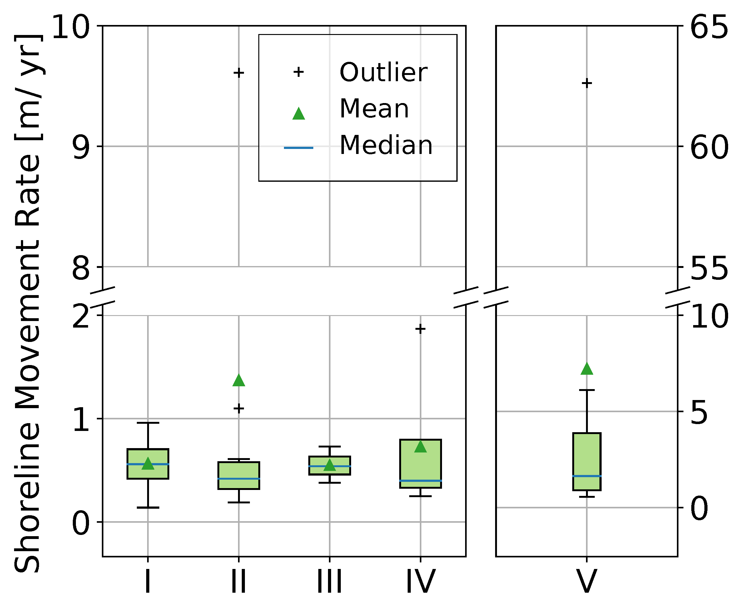
3.1.4. Deadhorse: Accuracy of Shoreline Movement Rates and Directions

At the Deadhorse study site, we sub-sampled 100 lakes and visually inspected them. Seven lakes had to be removed during this process since they were proven to be duplicates of already inspected lakes. Of the remaining 93 (100%) water bodies, a total of 70 (75%) were correctly mapped. For 41 (44%) of these accurately mapped water bodies, we could further derive a correct shoreline movement rate. The shoreline movement rate of the remaining 29 lakes was found to be incorrect. We discuss the error sources for this incorrect calculation of the shoreline movement rate and the matter of the duplicates further in Section 3.1.6.
Investigating the number of correctly and incorrectly derived shorelines of the inspected dataset (see Figure 4B), we find that minor movement rates of up to 0.40 m yr−1 showed an accuracy of 100% to 85%. They represented 29% (134 lakes) of the whole dataset (see Figure 4A). With higher movement rates, the accuracy declined. As soon as a value of 1.50 m yr−1 was exceeded, the number of correctly derived shoreline movement rates (34) almost equaled the number of incorrectly calculated rates (30). Examining the quality of the shoreline derivation for each lake size (see Figure 5C) category reveals a higher certainty of a correct movement rate calculation for lakes in Category V (>23 ha) with a value of 80%. Smaller lakes seemed more prone to a miscalculation, given the values of 60% to 70% of incorrectly identified shoreline movement rates.
The median rate of shoreline movement for lakes sized 0.10–0.36 ha was 0.56 m yr−1 (see Figure 5A). For lake size categories II to IV (0.36–23.04 ha), this ranged from a value of 0.40 to 0.54 m yr−1. Lakes larger than 23 ha showed a median movement rate of 1.64 m yr−1. The distributions of the correctly derived shoreline movement rates for each lake size category (see Figure A1) reveal that the median represents the range of values for size categories I (0.14–0.96 m yr−1), III (0.38–0.73 m yr−1) and IV (0.25–1.87 m yr−1) well. Size categories II and V, however, show a higher range of several (deca)meters.
As mentioned in Section 2.2.4, we derived net shoreline movement rates. Examining the corresponding water surface area changes (compared to the preceding time step), we found that the lakes of size categories I and V showed the highest variability in our study region. The water surface area changes were generally higher for size categories I and V (ranging from −20% to +30%, see inset map of Figure A2) with maximum values of 105–308% in water surface area gain (see Figure A2). The lakes of the remaining size categories showed only little variation in water surface area changes (−5 to +5%) accompanied by small movement rates (<1.0 m yr−1). High shoreline movement rates in combination with a high gain/loss in water surface area could only be observed in two cases: a shoreline movement rate of 9.61 m yr−1 and 62.6 m yr−1 and a water surface area change of −54% and −50%, respectively (seen as outliers in size categories II and V of Figure A1. Without exception, the high values of the shoreline movement rate and water surface area change originated from apparent water level changes suddenly connecting adjacent water bodies that were previously separate and vice versa, as explained more thoroughly in Section 3.1.6.
Examining the median annual shoreline movement rate for each time step revealed a rather consistent value of around 0.60 m yr−1 for all size classes: the specific values were 0.56 (2006–2010), 0.65 (2010–2013) and 0.54 m yr−1 (2013–2016).
The analysis of the valid lakes concerning a spatial pattern gives a clear result. The mean shoreline movement of more than 58% of the lakes was predominantly towards SE and S. Specifically, for 13 lakes (32%), the shoreline moved towards SE, while for 11 (27%), the shoreline moved towards S. Further prominent directions were SW (19%) and E (22%). This pattern persisted for lakes sized 0.10–0.36 ha and >23.04 ha (Figure 5B). Within the other size categories, no clear trend was found, mostly due to the small sample size of 41 water bodies for which a correct shoreline movement rate could be derived. A look at the movement direction in each time step depicts clear trends. While between the years 2006 and 2010, a predominant shoreline movement direction of SE was observed, the shoreline progressed in a SW/S direction for the next time step and shifted to E in the time span from 2013 to 2016. During the visual inspection, a spatial offset of approximately 1–3 pixels (0.50–1.50 m) was observed at some lakes in a NW direction for years 2006–2010 and 2013–2016, and an offset in a SW direction was observed for 2010–2013.

3.1.5. MP 396: Water Body Detection

At the site close to MP 396, only the water body detection scheme was verified. The workflow identified 66 water bodies, where almost half of them (31) turned out to be part of the river bed and floodplain of the Sagavanirktok River. In total, 63% of the derived shorelines corresponding to lakes were correctly identified. In particular, the shoreline derivation of the oxbow lakes close to the Dalton Highway worked very well (Figure 3B). The detection of water bodies as part of drained thaw lake basins, however, often led to an underestimation of the water surface due to shallow lake depths, as already observed at the Deadhorse study site.

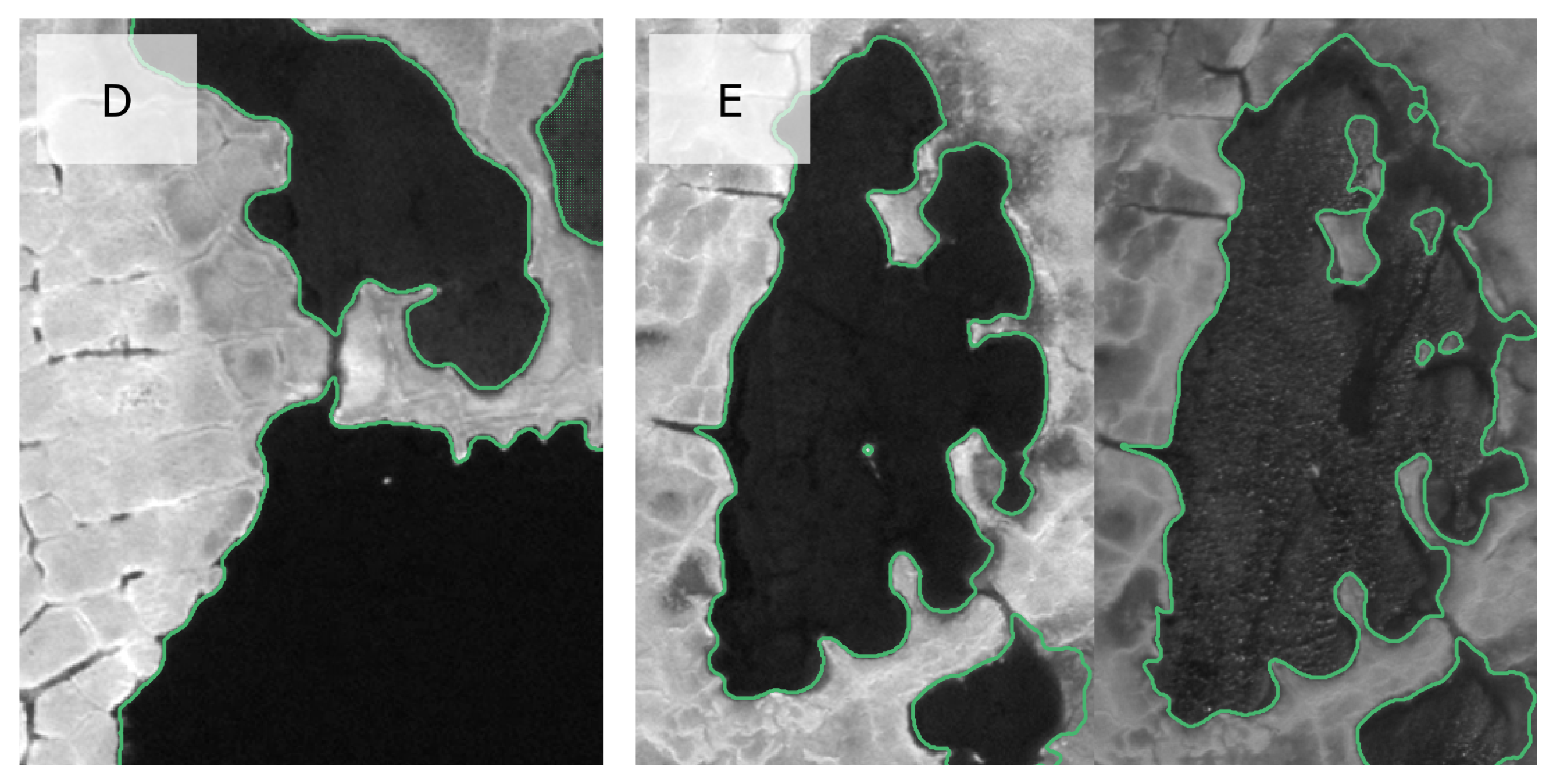
3.1.6. Identification of Error Sources

During the visual inspection, seven out of 100 sub-sampled lakes at the Deadhorse study site were identified as duplicates (see Figure A3A of the Appendix A). This was due to an apparent water level change between the time steps. Two adjacent lakes that were detected in 2006 under much drier conditions were suddenly connected by water-filled patches and ponds in the next time step. This led to an increase in the water surface area and shoreline movement for each of the former lakes. In 2013 and 2016, when the lake split up again, the calculation was done for each of the lake IDs, causing a duplicate.
Generally, we identified four different types of error sources, rendering the water body detection and/or the subsequent derivation of shoreline movement rate incorrect (for a visual impression, please refer to the Appendix A, Figure A3):
i
Distortion in the shore area due to sediment entry or shallow water depths results in an underestimation of the water surface area, and therefore the erroneous calculation of the lake shoreline movement rate, when the water surface area is fully identified in the next time step and vice versa (category: shore area);
ii
Speckle from sunglint leads to an underestimation of the water surface area. (category: sunglint);
iii
Undetected connections between adjacent lakes through water-filled patches, troughs of polygonal tundra or erosion and drainage gullies lead to the classification of several smaller lakes instead of one large lake (category: connectivity);
iv
Seasonal variations in water surface area. Depending on the amount of precipitation preceding the image acquisition, areas might appear as water bodies in one time step but as land in the next or vice versa. This can also lead to an overestimation of water surface area and therefore the incorrect derivation of shoreline geometry, when some moist patches are classified as (part of the) water bodies (category: water level).
At the Deadhorse study site, for 70% (16) of the incorrectly detected water bodies, we observed an underestimation of the water surface area caused by sediment input and visible lake bottoms in the shoreline area, rendering also the subsequent analysis of the shoreline movement rate incorrect (see Table 3). When looking at the incorrectly derived shoreline movement rates, 75% (39) of the water bodies showed these error sources. This means that an additional 23 shoreline movement rates were incorrect, although the initial water body detection was correct in the previous time step.
The same applies to the underestimation of the water surface area caused by sunglint. As outlined in Section 3.1.2, the median filter performed well for deep lakes and at the center of shallow lakes. However, it reached its limit in the shoreline area. We observed this kind of noise from sunglint (see the lake in the northeast corner of Figure 3A) in over a third (35%) of all inaccurately mapped water bodies and almost two thirds (63%) of the false shoreline movement rates.
As described in Section 3.1.4, lakes sized 0.10–0.36 ha seemed especially prone to a miscalculation. For 83% of these small lakes, a shoreline derivation failed due to an underestimation of the water surface area caused by lake bottom visibility (shallow water depths) while sunglint was responsible for 39% of the failed derivations.
A fourth of the incorrectly mapped water bodies lacked the identification of connections between lakes.
In the 2016 imagery of study site MP 396, no speckle from sunglint appeared. While 40% (see Table 3) of the incorrectly mapped water bodies showed distortion in the shoreline area and shallow water depths, the main error source (53%) was the overestimation of the water surface area by classifying moist patches as lakes. At this side, only 7% of the water bodies presented unidentified connections between the (oxbow) lakes.

4. Discussion

The proposed workflow successfully detected water bodies and delineated their shorelines with multi-temporal high-resolution imagery. The approach is fast and allows for easy adaptation to a user’s needs; e.g., focusing on specific sizes of water bodies or using alternative datasets for filtering misclassifications associated for example with infrastructure. The detection of shoreline movement rates worked best for sub-meter movement values (<0.4 m yr−1) with a probability of about 85% of correct shoreline derivation. At the Deadhorse study site, the largest sources of error leading to an incorrect mapping of water bodies were impurities of the spectral signal along the shore areas either caused by high sediment loads or lake bottom visibility. This was also valid for the falsely derived shoreline movement rates (occurring in 75% of the water bodies). Another important error source was the speckle from sunglint, which resulted in an underestimation of the water surface area (and false shoreline geometry), falsifying 63% of the incorrectly derived shoreline movement rates and more than a third of the falsely mapped water bodies. At mile post 396, the main error sources were an overestimation of moist patches (53%) as water bodies and the distortion from lake bottom visibility (40%).
In general, the derived range of shoreline movement rates agrees with the observed rates reported by other remote sensing and field observation-based local studies in Alaska [8,12,18] with comparable climate and permafrost conditions, but with slightly higher values in the small and mid-size lake categories and substantially higher rates for lakes >23 ha.
A unusually high movement rate of 62.6 m yr−1 (Figure 4B) associated with a lake shrinkage (of 50%) originated from water level changes. Low-lying shores were inundated in the former time step (2010) but dried up in the next (2013). Even minor changes in precipitation and evaporation can result in significant variations in the surface water area of some individual lakes depending on shore morphology. The different shoreline sensitivities towards water balance changes may further be related to catchment morphology and lake bathymetry. For example, the visual inspection suggests rather dry conditions in 2006 and 2013, exhibiting dry to moist patches and polygonal troughs in the first time step that were then filled with water during apparently overall wetter surface conditions in the next time step. On the other hand, lakes connected by troughs in 2010 shrunk to half their size in the next time step due to drier conditions. Both examples resulted in high apparent shoreline movement rates which in fact indicate seasonal fluctuations of water levels in the study area. Thus, when investigating annual shoreline changes, it is important to carefully consider the date of satellite images as well as previous weather conditions. In order to avoid strong water level fluctuations attributed to seasonal dynamics such as the thawing of the active layer, it is advisable to select images with acquisition dates late in the summer season when a maximum active layer thickness is reached. Furthermore, lake shoreline erosion presumably peaks later in the summer season when the maximum thaw depth intersects with increased wave action and strong precipitation, which also means that image acquisition should be performed late in the thawing season. With intra-seasonal temporally high resolution imagery, it would be possible to use the workflow also for the monitoring of seasonal water level changes and thus the assessment of landscape-scale lake water balance dynamics. Both intra-seasonal and annual analyses would benefit from further incorporating information on precipitation and temperature conditions in order to evaluate their influence on the water level during the image acquisition. Additionally integrating information on prevailing wind directions and velocities might furthermore give an explanation of the derived mean shoreline movement in SE and S directions: cross-winds can form strong currents that are able to predominantly erode parts of the shoreline [42] and may add to the thermal erosion. In future applications of the workflow across larger regions, including this meteorological data could also contribute to the understanding of environmental driving factors responsible for shoreline changes. In areas with low ice content, these processes might even be the main driver of lake expansion [43].
While the median filter works well for most time steps, it was clearly insufficient in 2010 and 2016. The radius was set after it had been tested on a small subset of the imagery. The error source category Sunglint accounted for 75% of the incorrectly derived shoreline movement rates; in half of the cases, it occurred in the shoreline area. To enhance the quality of the filter results, we recommend implementing an estimation of the noise density within the workflow. The median filtering could then be automatically applied to the derived threshold of the image noise. Further, the probability of sunglint occurrence might be estimated by implementing an automated extraction of the image acquisition angle and cloud coverage from the image metadata and information on wind speed from nearby weather stations. Another option is to use image products with a shortwave infrared (SWIR) band that is less vulnerable to sunglint [38], which was not available for our study. Using additional spectral bands may also increase the accuracy of mapping small, shallow water bodies and reduce the risk of overestimating moist patches by calculating enhanced water surface indexes [44,45,46]. Thus, the advantage of using very high resolution satellite images for the derivation of short-term shoreline movements of small lakes (<1.44 ha) could reach an even higher potential.
We observed two issues regarding the input data in this study. Firstly, in every image of the Deadhorse site, one specific lake (Lake Colleen) was filtered out since one of the industrial landuse polygons supposedly intersected with it. This resulted from minor geometrical inaccuracies in the OSM database. OpenStreetMap provides data that are mapped by a huge community of users dedicated to open-source and freely available datasets. Naturally, minor inaccuracies occur during the measurements since users operate devices with insufficient precision and lack access to restricted areas. As anticipated, official infrastructure data provided by official state agencies would increase the quality of the filtering. A rerun with a manually enhanced infrastructure map corrected this error.
Secondly, inferred movement rates and directions were partly affected by a slight offset that originated from different sensor characteristics and was linked to image rectification accuracy. It occurred throughout all time steps and could not be removed completely with the orthorectification of the imagery. However, the quality of the input data may be enhanced by using current high resolution digital elevation models (DEM) from LiDAR etc. for a better orthorectification. Furthermore, future improvements in satellite sensor technologies and image pre-processing may provide more accurate image alignment, which would greatly improve time series analysis in the automated workflow. Both input data issues add to the current limitations in automatizing the whole workflow and need to be addressed in the further development of this approach.
However, while preceding studies (see Section 1) significantly contributed to the enhancement of water body mapping approaches and the analysis of their temporal changes, our workflow is singular in providing an automated and therefore highly scalable process of extracting detailed shoreline movement rates from multi-temporal satellite images. Furthermore, tools which, similar to our workflow, derive movement rates on the basis of shoreline vector datasets, such as the Digital Shoreline Analysis System (DSAS) [47], do not derive the water bodies automatically. In addition, our workflow is based on open-source and free Python libraries, which can be run on all operating systems. These are necessary prerequisites in order to facilitate the upscaling of lake shoreline analyses spatially (regional to pan-Arctic) and temporally (from low decadal resolution to high sub-annual resolution) with the rapidly growing archives of high resolution satellite imagery.

5. Conclusions and Outlook

We present a largely automated and scalable workflow using multi-temporal sub-meter resolution remote sensing imagery, which is capable of mapping water bodies in tundra landscapes and providing shoreline movement rates and directions with certain accuracy limitations. We provide a quantification of the error sources leading to an incorrect shoreline detection which are predominantly caused by water surface area underestimation originating from shallow lake depths and sunglint. Future workflow developments will need to focus on the automated and reliable detection of these error sources to ensure a reliable quantification of water body changes. Furthermore, the presented workflow would strongly benefit from specific enhancements in data pre-processing regarding location accuracy during image orthorectification, the availability of filter datasets such as up-to-date infrastructure maps and an enhanced noise filtering, taking into account image metadata and weather station data. Despite current limitations, we argue that the presented workflow is highly scalable. It allows for the spatio-temporal quantification of water body changes across larger regions if the required imagery is available and erroneous shoreline detection can be filtered. With further clearly identified improvements, broad-scale water body detection and shoreline movement rate derivation at a high spatial and temporal resolution could be feasible. The workflow would also be useful for monitoring intra-seasonal lake level changes. The general approach has the potential to work across different spatial resolutions and scales, thus promising a fast and easy-to-use analysis tool for ongoing lake shoreline monitoring challenges. A pan-Arctic application of the water body detection part of the code using very high resolution imagery from Digital Globe is currently being realized through a collaboration with the Permafrost Discovery Gateway project (https://arcticdata.io/catalog/portals/permafrost (accessed on 15 July 2021)).

Author Contributions

Conceptualization, S.K., G.G., J.B. and M.L.; methodology, S.K., G.G. and M.L.; software, S.K.; validation, S.K.; formal analysis, S.K., G.G., J.B. and M.L.; resources, M.L.; data curation, S.K., G.G. and M.L.; writing—original draft preparation, S.K.; writing—review and editing, S.K., G.G., J.B. and M.L.; visualization, S.K.; supervision, G.G., J.B. and M.L.; project administration, M.L.; funding acquisition, M.L., S.K. All authors have read and agreed to the published version of the manuscript.

Funding

This work was conducted within the young investigator group PermaRisk, which is funded by the German Federal Ministry of Education and Research (BMBF) under the funding reference number 01LN1709A. S.K. was additionally supported by a 2-year grant from Christiane Nüsslein-Volhard foundation and a stipend from a family fund of Humboldt-Universität, Berlin.

Data Availability Statement

Infrastructure map data are copyrighted by OpenStreetMap contributors, ODbL 1.0, and available from https://www.openstreetmap.org (accessed on 15 July 2021). The workflow code is available under https://github.com/CryoGrid/PyShore (accessed on 15 July 2021).

Acknowledgments

The authors would like to thank Sina Muster and Anna Liljedahl for their valuable suggestions and comments on this manuscript.

Conflicts of Interest

The authors declare no conflict of interest. The funders had no role in the design of the study; in the collection, analyses, or interpretation of data; in the writing of the manuscript, or in the decision to publish the results.

Abbreviations

The following abbreviations are used in this manuscript:
VHRVery high resolution
MPMile post
panPanchromatic
LiDARLight detection and ranging
RGBRed–green–blue
NIRNear infrared
SWIRShortwave infrared
OSMOpenStreetMap
yryear

Appendix A

Figure A1. Data distribution of annual shoreline movement rates for each lake size category. The green-colored boxes represent the interquartile range (25th to 75th percentile), while the whiskers show the minimum (25%-percentile − 1.5∗interquartile range) and maximum (75%-percentile + 1.5∗interquartile range) value of the data. Please note the different (and interrupted) y-axes for lake size categories I–IV and V for a better visualization.
Remotesensing 13 02802 g0a1
Figure A2. Scatter plot showing annual shoreline movement rates and the corresponding water surface area difference for each lake size category. The values within the red square are shown in the inset graph in the top right corner.
Remotesensing 13 02802 g0a2
Figure A3. Examples of error sources for the incorrect derivation of water bodies and/or shoreline movement rates. (A) The duplicates mentioned in Section 3.1.6. Subsequent images show the underestimation of water surface area due to shallow water depths (B), sunglint (C) and unidentified connections between lakes (D) and the overestimation by including adjacent moist patches (E) (Background high-resolution imagery copyrighted by DigitalGlobe, 2006 & 2013).
Remotesensing 13 02802 g0a3aRemotesensing 13 02802 g0a3b

References

  1. Grosse, G.; Jones, B.; Arp, C. Thermokarst Lakes, Drainage, and Drained Basins. In Treatise on Geomorphology; Shroder, J.F., Ed.; Academic Press: San Diego, CA, USA, 2013; pp. 325–353. [Google Scholar] [CrossRef]
  2. Muster, S.; Roth, K.; Langer, M.; Lange, S.; Cresto Aleina, F.; Bartsch, A.; Morgenstern, A.; Grosse, G.; Jones, B.; Sannel, A.B.K.; et al. PeRL: A circum-Arctic permafrost region pond and lake database. Earth Syst. Sci. Data 2017, 9, 317–348. [Google Scholar] [CrossRef] [Green Version]
  3. Rautio, M.; Dufresne, F.; Laurion, I.; Bonilla, S.; Vincent, W.F.; Christoffersen, K.S. Shallow freshwater ecosystems of the circumpolar Arctic. Ecoscience 2011, 18, 204–222. [Google Scholar] [CrossRef]
  4. Pienitz, R.; Doran, P.T.; Lamoureux, S.F. Origin and geomorphology of lakes in the polar regions. In Polar Lakes and Rivers: Limnology of Arctic and Antarctic Aquatic Ecosystems, 1st ed.; Vincent, W.F., Laybourn-Parry, J., Eds.; Oxford University Press: Oxford, UK, 2008; pp. 25–42. [Google Scholar]
  5. Brosius, L.; Anthony, K.W.; Treat, C.; Lenz, J.; Jones, M.; Bret-Harte, M.; Grosse, G. Spatiotemporal patterns of northern lake formation since the Last Glacial Maximum. Quat. Sci. Rev. 2021, 253, 106773. [Google Scholar] [CrossRef]
  6. Langer, M.; Westermann, S.; Boike, J.; Kirillin, G.; Grosse, G.; Peng, S.; Krinner, G. Rapid degradation of permafrost underneath waterbodies in tundra landscapes—Toward a representation of thermokarst in land surface models. J. Geophys. Res. Earth Surf. 2016, 121, 2446–2470. [Google Scholar] [CrossRef]
  7. Muster, S.; Riley, W.J.; Roth, K.; Langer, M.; Cresto Aleina, F.; Koven, C.D.; Lange, S.; Bartsch, A.; Grosse, G.; Wilson, C.J.; et al. Size distributions of Arctic waterbodies reveal consistent relations in their statistical moments in space and time. Front. Earth Sci. 2019, 7, 5. [Google Scholar] [CrossRef] [Green Version]
  8. Jorgenson, M.T.; Shur, Y. Evolution of lakes and basins in northern Alaska and discussion of the thaw lake cycle. J. Geophys. Res. Earth Surf. 2007, 112, 1–12. [Google Scholar] [CrossRef]
  9. Arp, C.D.; Jones, B.M. Geography of Alaska Lake Districts: Identification, Description, and Analysis of Lake-Rich Regions of a Diverse and Dynamic State; U.S. Geological Survey Scientific Investigations Report 2008-5215; US Geological Survey: Menlo Park, CA, USA, 2009; p. 40.
  10. Walter Anthony, K.; Daanen, R.; Anthony, P.; Schneider Von Deimling, T.; Ping, C.L.; Chanton, J.P.; Grosse, G. Methane emissions proportional to permafrost carbon thawed in Arctic lakes since the 1950s. Nat. Geosci. 2016, 9, 679–682. [Google Scholar] [CrossRef]
  11. In’t Zandt, M.H.; Liebner, S.; Welte, C.U. Roles of Thermokarst Lakes in a Warming World. Trends Microbiol. 2020, 28, 769–779. [Google Scholar] [CrossRef] [PubMed]
  12. Jones, B.M.; Grosse, G.; Arp, C.D.; Jones, M.C.; Walter Anthony, K.M.; Romanovsky, V.E. Modern thermokarst lake dynamics in the continuous permafrost zone, northern Seward Peninsula, Alaska. J. Geophys. Res. Biogeosci. 2011, 116, 1–13. [Google Scholar] [CrossRef]
  13. Carroll, M.L.; Townshend, J.R.G.; Dimiceli, C.M.; Loboda, T.; Sohlberg, R.A. Shrinking lakes of the Arctic: Spatial relationships and trajectory of change. Geophys. Res. Lett. 2011, 38, 1–5. [Google Scholar] [CrossRef] [Green Version]
  14. Olthof, I.; Fraser, R.H.; Schmitt, C. Landsat-based mapping of thermokarst lake dynamics on the Tuktoyaktuk Coastal Plain, Northwest Territories, Canada since 1985. Remote Sens. Environ. 2015, 168, 194–204. [Google Scholar] [CrossRef]
  15. Smith, L.C.; Sheng, Y.; MacDonald, G.M.; Hinzman, L.D. Atmospheric Science: Disappearing Arctic lakes. Science 2005, 308, 1429. [Google Scholar] [CrossRef] [Green Version]
  16. Nitze, I.; Grosse, G.; Jones, B.M.; Arp, C.D.; Ulrich, M.; Fedorov, A.; Veremeeva, A. Landsat-based trend analysis of lake dynamics across Northern Permafrost Regions. Remote Sens. 2017, 9, 640. [Google Scholar] [CrossRef] [Green Version]
  17. Riordan, B.; Verbyla, D.; McGuire, A.D. Shrinking ponds in subarctic Alaska based on 1950–2002 remotely sensed images. J. Geophys. Res. Biogeosci. 2006, 111. [Google Scholar] [CrossRef]
  18. Arp, C.D.; Jones, B.M.; Urban, F.E.; Grosse, G. Hydrogeomorphic processes of thermokarst lakes with grounded-ice and floating-ice regimes on the Arctic coastal plain, Alaska. Hydrol. Process. 2011, 25, 2422–2438. [Google Scholar] [CrossRef]
  19. Sannel, A.B.K.; Brown, I.A. High-resolution remote sensing identification of thermokarst lake dynamics in a subarctic peat plateau complex. Can. J. Remote Sens. 2010, 36, S26–S40. [Google Scholar] [CrossRef]
  20. Farquharson, L.M.; Romanovsky, V.E.; Cable, W.L.; Walker, D.A.; Kokelj, S.V.; Nicolsky, D. Climate Change Drives Widespread and Rapid Thermokarst Development in Very Cold Permafrost in the Canadian High Arctic. Geophys. Res. Lett. 2019, 46, 6681–6689. [Google Scholar] [CrossRef] [Green Version]
  21. Liljedahl, A.K.; Boike, J.; Daanen, R.P.; Fedorov, A.N.; Frost, G.V.; Grosse, G.; Hinzman, L.D.; Iijma, Y.; Jorgenson, J.C.; Matveyeva, N.; et al. Pan-Arctic ice-wedge degradation in warming permafrost and its influence on tundra hydrology. Nat. Geosci. 2016, 9, 312–318. [Google Scholar] [CrossRef]
  22. Shah, C.A. Automated lake shoreline mapping at subpixel accuracy. IEEE Geosci. Remote Sens. Lett. 2011, 8, 1125–1129. [Google Scholar] [CrossRef]
  23. Sheng, Y.; Shah, C.A.; Smith, L.C. Automated image registration for hydrologic change detection in the lake-rich arctic. IEEE Geosci. Remote Sens. Lett. 2008, 5, 414–418. [Google Scholar] [CrossRef]
  24. Bangira, T.; Alfieri, S.M.; Menenti, M.; van Niekerk, A. Comparing thresholding with machine learning classifiers for mapping complex water. Remote Sens. 2019, 11, 1351. [Google Scholar] [CrossRef] [Green Version]
  25. Otsu, N. A Threshold Selection Method from Gray-Level Histograms. IEEE Trans. Syst. Man Cybern. 1979, 9, 62–66. [Google Scholar] [CrossRef] [Green Version]
  26. Tian, B.; Li, Z.; Zhang, M.; Huang, L.; Qiu, Y.; Li, Z.; Tang, P. Mapping Thermokarst Lakes on the Qinghai-Tibet Plateau Using Nonlocal Active Contours in Chinese GaoFen-2 Multispectral Imagery. IEEE J. Sel. Top. Appl. Earth Obs. Remote Sens. 2017, 10, 1687–1700. [Google Scholar] [CrossRef]
  27. Cooley, S.W.; Smith, L.C.; Stepan, L.; Mascaro, J. Tracking Dynamic Northern Surface Water Changes with High-Frequency Planet CubeSat Imagery. Remote Sens. 2017, 9, 1306. [Google Scholar] [CrossRef] [Green Version]
  28. Cooley, S.W.; Smith, L.C.; Ryan, J.C.; Pitcher, L.H.; Pavelsky, T.M. Arctic-Boreal Lake Dynamics Revealed Using CubeSat Imagery. Geophys. Res. Lett. 2019, 46, 2111–2120. [Google Scholar] [CrossRef]
  29. Nitze, I.; Cooley, S.W.; Duguay, C.R.; Jones, B.M.; Grosse, G. The catastrophic thermokarst lake drainage events of 2018 in northwestern Alaska: Fast-forward into the future. Cryosphere 2020, 14, 4279–4297. [Google Scholar] [CrossRef]
  30. Brown, J.; Ferrians, O.J.; Heginbottom, J.A.; Melnikov, E.S. Circum-Arctic Map of Permafrost and Ground-Ice Conditions; Digital Media, National Snow and Ice Data Center: Boulder, CO, USA, 2001. [Google Scholar]
  31. NOAA National Centers for Environmental Information. 1981-2010 Normals | Data Tools | Climate Data Online (CDO) | National Climatic Data Center (NCDC). 2021. Available online: https://www.ncdc.noaa.gov/cdo-web/datatools/normals (accessed on 26 May 2021).
  32. Walker, D.; Raynolds, M.K. Circumpolar Arctic Vegetation, Geobotanical, Physiographic Maps, 1982–2003; ORNL DAAC: Oak Ridge, TN, USA, 2018. [Google Scholar] [CrossRef]
  33. Sellmann, P.V.; Brown, J.; Lewellen, R.I.; McKim, H.; Merry, C. The Classification and Geomorphic Implications of Thaw Lakes on the Arctic Coastal Plain, Alaska; Cold Regions Research and Engineering Laboratory: Hanover, NH, USA, 1975. [Google Scholar]
  34. Hinkel, K.M.; Frohn, R.C.; Nelson, F.E.; Eisner, W.R.; Beck, R.A. Morphometric and spatial analysis of thaw lakes and drained thaw lake basins in the western Arctic Coastal Plain, Alaska. Permafr. Periglac. Process. 2005, 16, 327–341. [Google Scholar] [CrossRef]
  35. Raynolds, M.K.; Walker, D.A.; Ambrosius, K.J.; Brown, J.; Everett, K.R.; Kanevskiy, M.; Kofinas, G.P.; Romanovsky, V.E.; Shur, Y.; Webber, P.J. Cumulative geoecological effects of 62 years of infrastructure and climate change in ice-rich permafrost landscapes, Prudhoe Bay Oilfield, Alaska. Glob. Chang. Biol. 2014, 20, 1211–1224. [Google Scholar] [CrossRef]
  36. OpenStreetMap Contributors and Geofabrik GmbH. Geofabrik Download Server. 2018. Available online: http://download.geofabrik.de/ (accessed on 15 July 2021).
  37. Garaba, S.P.; Schulz, J.; Wernand, M.R.; Zielinski, O. Sunglint detection for unmanned and automated platforms. Sensors 2012, 12, 12545–12561. [Google Scholar] [CrossRef]
  38. Wang, Z.; Liu, J.; Li, J.; Zhang, D.D. Multi-Spectral Water Index (MuWI): A Native 10-m Multi-Spectral Water Index for Accurate Water Mapping on Sentinel-2. Remote Sens. 2018, 10, 1643. [Google Scholar] [CrossRef] [Green Version]
  39. van der Walt, S.; Schönberger, J.L.; Nunez-Iglesias, J.; Boulogne, F.; Warner, J.D.; Yager, N.; Gouillart, E.; Yu, T.; The Scikit-Image Contributors. Scikit-image: Image processing in Python. PeerJ 2014, 2, e453. [Google Scholar] [CrossRef]
  40. Lillesand, T.M.; Kiefer, R.W.; Chipman, J.W. Remote Sensing and Image Interpretation, 6th ed.; Wiley: Hoboken, NJ, USA, 2008; p. 756. [Google Scholar]
  41. Lara, M.J.; Chipman, M.L.; Hu, F.S. Automated detection of thermoerosion in permafrost ecosystems using temporally dense Landsat image stacks. Remote Sens. Environ. 2019, 221, 462–473. [Google Scholar] [CrossRef]
  42. Côté, M.M.; Burn, C.R. The oriented lakes of Tuktoyaktuk Peninsula, Western Arctic Coast, Canada: A GIS-based analysis. Permafr. Periglac. Process. 2002, 13, 61–70. [Google Scholar] [CrossRef]
  43. Wolfe, S.; Murton, J.; Bateman, M.; Barlow, J. Oriented-lake development in the context of late Quaternary landscape evolution, McKinley Bay Coastal Plain, western Arctic Canada. Quat. Sci. Rev. 2020, 242, 106414. [Google Scholar] [CrossRef]
  44. Xu, H. Modification of normalised difference water index (NDWI) to enhance open water features in remotely sensed imagery. Int. J. Remote Sens. 2006, 27, 3025–3033. [Google Scholar] [CrossRef]
  45. Korzeniowska, K.; Korup, O. Object-based detection of lakes prone to seasonal ice cover on the Tibetan Plateau. Remote Sens. 2017, 9, 339. [Google Scholar] [CrossRef] [Green Version]
  46. Feyisa, G.L.; Meilby, H.; Fensholt, R.; Proud, S.R. Automated Water Extraction Index: A new technique for surface water mapping using Landsat imagery. Remote Sens. Environ. 2014, 140, 23–35. [Google Scholar] [CrossRef]
  47. Himmelstoss, E.A.; Henderson, R.E.; Kratzmann, M.G.; Farris, A.S. Digital Shoreline Analysis System (DSAS) Version 5.0 User Guide; Open-File Report 2018-1179; US Geological Survey: Menlo Park, CA, USA, 2018; p. 126.
Figure 1. Illustration of all processing steps, subdivided into data input, manual pre-processing and the automated workflow with the resulting output. The automated part consists of (i) the buffering of linear infrastructure elements and merging with polygonal features, (ii) image noise removal, (iii) water body classification and the vectorization of the shoreline geometry, (iv) filtering for a user-defined water body size and elimination of infrastructure elements, (v) nearest neighbor analysis for each vertex and (vi) the subsequent derivation of movement rates and directions.
Remotesensing 13 02802 g001
Figure 2. Subfigure (A) shows Sentinel-2 near-infrared (NIR) images (Band 8 at 842 nm, acquisition on 23 July 2019) of the study sites (marked with red squares) on the North Slope of Alaska. Detailed area subset with thermokarst lakes near the linear infrastructure in Deadhorse (B) and oxbow lakes at mile post 396 of the Dalton Highway (C). High-resolution imagery is the pan-sharpened NIR band of Quickbird-2 and WorldView-2, respectively (Copyright: DigitalGlobe, 2006 & 2016).The underlying world border dataset for the inset map of Alaska in (A) is available from http://thematicmapping.org/ (accessed on 26 June 2021) and licensed under CC BY-SA 3.0 https://creativecommons.org/licenses/by-sa/3.0/ (accessed on 26 June 2021).
Remotesensing 13 02802 g002
Figure 3. (A,B) Results of water body detection (orange lines) overlaid by water bodies after filtering of infrastructure and size (green lines). (C) A schematic drawing of the nearest-point analysis. For each vertex of the polygon, the nearest vertex (red arrow) of the temporally subsequent polygon is identified. The distance and direction are calculated using trigonometric functions.
Remotesensing 13 02802 g003
Figure 4. Histogram of all 470 lakes (in percent) at the Deadhorse study site (A) for each mean annual shoreline movement rate and corresponding (B) number of correctly (green) and falsely (blue) derived shorelines of the inspected sub-sample dataset. Please note that the logarithmic scale (labeled at the top of the x-axis) is divided into seven sub-classes (labeled at the bottom of the x-axis).
Remotesensing 13 02802 g004
Figure 5. Median annual shoreline movement rate (A) and dominant movement directions (B) for each lake size category of the sub-sampled dataset at Deadhorse study site. Graph (C) shows the quality of the shoreline derivation for each lake size.
Remotesensing 13 02802 g005
Table 1. Image acquisition date, spatial resolution of the multi-spectral and panchromatic bands and sensor type.
Acquisition Date
[mm/dd/yyyy]
Spatial Resolution [m]Sensor
Deadhorse
08/15/20062.8 m0.7 mQuickbird-2
07/09/20102.0 m0.5 mWorldView-2
07/16/20132.0 m0.5 mWorldView-2
07/10/20162.0 m0.3 mWorldView-3
Dalton Highway MP 396
08/27/20162.0 m0.5 mWorldView-2
Table 2. Total number of derived water bodies at both study sites, broken down into the five lake size categories. Water bodies were labeled “detected” if they occurred in both years of the analyzed time step at the Deadhorse study site. Water bodies labeled as empty represent the number of lakes that were only detected in the first year. A total of 109 lakes occurred throughout all the time steps.
DeadhorseMP 396
2006–20102010–20132013–20162016
Detection20523322766
Empty317391
0.10–0.36 ha87624839
0.36–1.44 ha58525815
1.44–5.76 ha1625126
5.76–23.04 ha5656
>23.04 ha815130
Total17416013666
In every time step 109
Table 3. Major error sources identified for an incorrect mapping of water bodies and calculation of shoreline movement rate. Note that water bodies show multiple reasons for an incorrect detection; therefore, the values do not add up to 100%.
Category Error SourcesWater Body Detection IncorrectShoreline Movement Rate Incorrect
Deadhorse23 lakes52 lakes
Shore area 70 % 75 %
Sunglint 35 % 63 %
Connectivity 26 % 12 %
Water level 10 %
MP 39613 lakes
Shore area 40 %
Sunglint
Connectivity 7 %
Water level 53 %
Publisher’s Note: MDPI stays neutral with regard to jurisdictional claims in published maps and institutional affiliations.

