Mosaicking Landsat and Sentinel-2 Data to Enhance LandTrendr Time Series Analysis in Northern High Latitude Permafrost Regions


1
Alfred Wegener Institute for Polar and Marine Research, Telegrafenberg A 45, 14473 Potsdam, Germany
2
Institute of Geosciences, University of Potsdam, Karl-Liebknecht-Str. 24-25, 14476 Potsdam, Germany
*
Author to whom correspondence should be addressed.
†
Current address: Telegrafenberg A 45, 14473 Potsdam, Germany.
Remote Sens. 2020, 12(15), 2471; https://doi.org/10.3390/rs12152471
Submission received: 12 May 2020
/
Revised: 22 July 2020
/
Accepted: 29 July 2020
/
Published: 1 August 2020
(This article belongs to the Section Environmental Remote Sensing)
Abstract
:Permafrost is warming in the northern high latitudes, inducing highly dynamic thaw-related permafrost disturbances across the terrestrial Arctic. Monitoring and tracking of permafrost disturbances is important as they impact surrounding landscapes, ecosystems and infrastructure. Remote sensing provides the means to detect, map, and quantify these changes homogeneously across large regions and time scales. Existing Landsat-based algorithms assess different types of disturbances with similar spatiotemporal requirements. However, Landsat-based analyses are restricted in northern high latitudes due to the long repeat interval and frequent clouds, in particular at Arctic coastal sites. We therefore propose to combine Landsat and Sentinel-2 data for enhanced data coverage and present a combined annual mosaic workflow, expanding currently available algorithms, such as LandTrendr, to achieve more reliable time series analysis. We exemplary test the workflow for twelve sites across the northern high latitudes in Siberia. We assessed the number of images and cloud-free pixels, the spatial mosaic coverage and the mosaic quality with spectral comparisons. The number of available images increased steadily from 1999 to 2019 but especially from 2016 onward with the addition of Sentinel-2 images. Consequently, we have an increased number of cloud-free pixels even under challenging environmental conditions, which then serve as the input to the mosaicking process. In a comparison of annual mosaics, the Landsat+Sentinel-2 mosaics always fully covered the study areas (99.9–100 %), while Landsat-only mosaics contained data-gaps in the same years, only reaching coverage percentages of 27.2 %, 58.1 %, and 69.7 % for Sobo Sise, East Taymyr, and Kurungnakh in 2017, respectively. The spectral comparison of Landsat image, Sentinel-2 image, and Landsat+Sentinel-2 mosaic showed high correlation between the input images and mosaic bands (e.g., for Kurungnakh 0.91–0.97 between Landsat and Landsat+Sentinel-2 mosaic and 0.92–0.98 between Sentinel-2 and Landsat+Sentinel-2 mosaic) across all twelve study sites, testifying good quality mosaic results. Our results show that especially the results for northern, coastal areas was substantially improved with the Landsat+Sentinel-2 mosaics. By combining Landsat and Sentinel-2 data we accomplished to create reliably high spatial resolution input mosaics for time series analyses. Our approach allows to apply a high temporal continuous time series analysis to northern high latitude permafrost regions for the first time, overcoming substantial data gaps, and assess permafrost disturbance dynamics on an annual scale across large regions with algorithms such as LandTrendr by deriving the location, timing and progression of permafrost thaw disturbances.

1. Introduction
Permafrost is warming in the northern high latitudes [1], which has considerable impacts on Arctic terrestrial landscapes. Permafrost is ground that remains at or below 0 °C for at least two consecutive years and it covers roughly 25% of the northern hemisphere [2]. Being defined as a thermal state of the subsurface makes permafrost directly vulnerable to changes in the energy balance of the land surface, in particular the long-term changes in mean annual air temperature, precipitation regimes, and snow distribution and thickness that are currently observed across the high latitudes [3,4]. Continued warming causes widespread permafrost thaw, resulting ultimately in near-surface permafrost loss at local to regional scales [5]. Wide landscape changes can be associated with permafrost thaw and loss and have impacts on ecosystems [6,7], hydrological systems [8,9], soil carbon accumulation and decomposition [10], greenhouse gas emissions [11], and stability of infrastructure in permafrost areas [12]. Considering the vast area permafrost covers across the northern hemisphere and its strong linkages to the Arctic biophysical system [13], changes in the distribution of permafrost due to thaw is of high relevance for the Arctic amplification of global climate change [4,14].
To make more precise estimations of the impact of permafrost thaw on landscapes and biogeochemical cycles, a more detailed remote sensing-based assessment of permafrost disturbances is necessary. Many thaw-related permafrost disturbances in the northern latitudes such as thermokarst formation, thermokarst lake drainage, flooding, rapid soil erosion, and wildfires [15,16] can be tracked with remote sensing methods that provide key information on the distribution, magnitude, duration, and impacts of disturbances [17,18]. However so far, the extent of remotely sensed permafrost disturbance assessments are limited spatially and temporally. Abrupt permafrost disturbance features [15] have been mainly mapped on local to regional scales, such as retrogressive thaw slumps [18,19,20], fires [21], and lake changes [18]. These studies either derived disturbance dynamic parameters from few individual time snapshots [22,23,24,25], or determined trends across a period of time [18,19]. However, knowledge on the annual disturbance dynamics is required on regional to pan-arctic scales. This is crucial for identifying main drivers of abrupt thaw events and including these processes in large-scale climate models.
A number of remote sensing algorithms that were developed for land cover change and forest disturbance applications to detect landscape changes at regional to global scales, capture the temporal dynamics of disturbance features. Since the start of the open access policy of the Landsat data archive in 2008 [26], Landsat is often chosen for high spatial and temporal resolution land cover and change detection assessments. For example, Hansen et al. [27] presented a global forest gain and loss algorithm and Pekel et al. [28] a surface water assessment and its changes with Landsat data. Landsat has the longest available data record, covering more than 48 years, which presents a unique opportunity for long-term assessment studies. Landsat satellites are multispectral sensor systems, providing a spatial resolution of 30 m at nominal revisit times of 16 days covering the whole globe [29]. The Landsat archive therefore allows to assess processes at high spatial resolution and with a reliable continuous time series for more than several decades by now.
The most widely-used algorithms are the Landsat-based detection of Trends in Disturbance and Recovery (LandTrendr) [30], the vegetation change tracker (VCT) [31], the Break detection For Additive Season and Trend (BFAST monitor) [32], the Continuous Change Detection and Classification model (CCDC) [33], and the forest gain and loss algorithm by Hansen et al. (2013) [27], according to a compilation by Zhu (2017) [34] based on algorithm characteristics, such as temporal frequency, change indices, and gradual or abrupt change detection. They all have in common the smallest assessment unit as a pixel but differ in the required temporal data frequency, change index application, the form of disturbance they assess (gradual or abrupt), and whether they are used for near real-time monitoring or past change detection. Since data availability in the northern high latitudes is limited drastically by frequent cloud cover [35], most of the widely-used algorithms that require a very high temporal frequency of input data are not suitable for Arctic applications.
An exception is LandTrendr, as it creates yearly mosaics from cloud-free Landsat images by aggregating cloud-free pixels from a defined period of time, e.g., the summer months [30]. With this approach, LandTrendr ensures a continuous disturbance assessment with an annual resolution. Using aggregated data as input is a promising method to bypass data limitations in the northern high latitudes [36,37]. Moreover, LandTrendr is flexible in change index choice and captures both abrupt and gradual changes. LandTrendr applies a segmentation algorithm for change and trend detection to the time series of annual Landsat mosaics. The segmentation algorithm splits the time series into vertices, points of abrupt spectral change, and time stretches in between of vertices with change, no change or gradual trends, which then represent abrupt and gradual land cover change, respectively. The algorithm results provide information on the disturbance year, magnitude of change, and recovery duration [30]. Since 2018, LandTrendr is incorporated into Google Earth Engine (GEE) [38] and is therefore easily transferable to new application areas, benefiting from GEEs processing power and easily available large-scale satellite data sets [38]. The application of LandTrendr to the high latitudes would allow assessing permafrost disturbance processes for the first time with a continuous time series, deriving temporal dynamics on multiyear to annual scales, derived from more than 20 years of data, at high spatial resolution, which has not been achieved before.
However, even the annual LandTrendr mosaics, based on the moderate repeat frequency of Landsat images, contain considerable gaps due to lack of cloud-free images and pixels in some years, in particular at higher Arctic and coastal sites. Additional disadvantages include high latitude environmental factors such as frequent snow and ice cover, a short growing season length, and a challenging solar geometry [29,39]. As annual cloud- and gap-free mosaics are the prerequisite of a reliable and high-quality time series implementation such as LandTrendr, the single-sensor based algorithm remains prone to local and regional observation gaps in the high latitudes [40]. These are major challenges for permafrost disturbance studies as these same regions are also underlain by thaw vulnerable, ice-rich and organic-rich permafrost [2,41], where first local studies already show extensive permafrost thaw [24,25]. Hence, it is crucial to enhance the input database for a LandTrendr time series analysis for northern high latitude applications.
Active remote sensing sensors such as Synthetic Aperture Radar (SAR) sensors can penetrate clouds and do not rely on sun illumination. Therefore, they are less restricted by weather and illumination conditions, which is very useful in northern high latitudes [42]. Varying SAR methods have been applied to northern high latitudes for land cover mapping [43], surface deformation assessments in permafrost regions [44,45,46] and active layer thickness estimations [47]. While the range of application possibilities of SAR data is broad and promising, one major drawback is its overall sparse data availability due to irregular acquisition schemes from historical SAR sensors such as ERS-1/2 SAR, ALOS-1 PALSAR-1, TerraSAR-X and Radarsat-2 [48]. This has only changed recently since the launch of the Copernicus Sentinel-1 satellites in 2014 and 2016, and their short image acquisition rate in polar areas every 6 to 12 days [49]. With five years of continuous temporally high-resolution data, the available time series for landscape analysis from Sentinel-1 is comparably short and hence the longer optical remote sensing time series of Landsat is still the preferred choice for long time series analysis assessments as exemplified here.
We here propose to combine Landsat and Sentinel-2 images in the mosaicking workflow to ensure data coverage for a continuous time series and a reliable input basis for change assessment algorithms, such as LandTrendr. The Sentinel-2 system has a comparable sensor to Landsat but consists of two near-identical satellites, which have a combined revisit time of only five days [50]. Combining Landsat 8 and Sentinel-2 shortens the overall revisit time in the northern high latitudes drastically, increasing the likelihood of obtaining good quality, cloud-free images [51] and potentially enhancing the database for large scale mosaics [52]. The two sensors are overall compatible and spectral band adjustment coefficients ensure high spectral comparability [53,54], which are also available for Arctic-Boreal regions specifically [55]. Therefore, with the launch of the first Sentinel-2 satellite (Sentinel-2A) there is large potential to improve the annual cloud- and gap-free mosaics from the second half of 2015 onward.
Despite the availability of already existing harmonised Landsat/Sentinel-2 products, such as the Harmonized Landsat and Sentinel-2 surface reflectance data set [54], the Landsat+Sentinel-2 analysis ready data [56] or Sen2Like, a tool to generate Sentinel-2 harmonised surface reflectance products with other sensors [57], these global data sets often show discrepancies to regionally derived and adjusted products [53,55,58]. Hence, a regionally fitted harmonisation approach is favoured for regional applications.
The overall objective of this study is to assess the combination of Landsat and Sentinel-2 data to create good quality mosaics for northern high latitudes as input for high temporal assessment applications such as LandTrendr in GEE. To address this main objective, we focus on three sub-objectives: (1) adapting a mosaicking workflow to incorporate both Landsat and Sentinel-2 images; (2) evaluating the improved data availability as a basis for annual mosaics when using Landsat and Sentinel-2 data; and (3) demonstrating the Landsat+Sentinel-2 mosaic coverage improvements and the preservation of good mosaic quality. We apply and test this framework to twelve diverse study sites in the high latitude permafrost regions across northern Siberia.
2. Materials and Methods
2.1. Study Sites
This assessment focuses on the terrestrial northern high latitudes and in particular on northern Siberia. We selected twelve study sites, spanning from Taymyr Peninsula in the west (80°E) to Chukotka Peninsula in the east (172°W) and from the northern margins of the Siberian mainland (77°N) to central Yakutia in the south (61°N) (Figure 1). The study sites exemplify a variety of landscapes and cover the range of climatic, geologic, geomorphologic and vegetational conditions in the North Siberian permafrost regions. While all sites except Chukotka are within the continuous permafrost zone [2], we included sites which are inland or coastal, with various terrain specifications and elevation levels, within the taiga or tundra ecoregion [59], and with different ground ice contents and thus thaw vulnerability (Table 1). Climatically the study sites lie within the arctic to boreal climate zones and in both maritime and continental areas which defines the rather broad climate region of northern Siberia [60]. The mean annual air temperature (MAAT) for January and July and mean annual total precipitation (MATP) values were extracted from ERA5 data for each study site [61]. Furthermore, specific study sites were chosen as they accommodate long field data records and represent frequently visited research areas, such as the Lena Delta, Batagay, Chokurdakh and the Pleistocene Park near Cherskiy.
For our analysis, we defined each study site by determining a centre point and a 25 × 25 km square area around the centre point. From here on, the term study site refers to the general study location while the term AOI refers to the coordinates of the centre point in our processing workflow (Section 2.3) and AOIarea to the 25 × 25 km areal (Section 2.5) extent of every study site. So, every study site consists of an AOI and an AOIarea.
2.2. Data
In our study, we worked with Landsat and Sentinel-2 data. The Landsat program is the longest running civilian optical remote sensing operation, continuously acquiring images of our Earth since 1972. Temporally overlapping missions ensured data continuity for more than 48 years already [62]. The missions’ sensors changed moderately over the years but general specifications sustained. Landsat satellites are sun-synchronous, polar-orbiting and have a repeat cycle of 16 days at the equator. The Landsat sensors are multi-spectral imagers, covering a wide range of the electromagnetic wavelength spectrum with their bands, from visible to thermal infrared, and acquiring images with 30 m spatial resolution [63]. In 2015 and 2017, the European Space Agency (ESA) launched the Sentinel-2 satellites from their Copernicus program. The Sentinel-2 mission, consisting of two nearly identical satellites, Sentinel-2A and Sentinel-2B, also operates multi-spectral instruments. Like Landsat, the Sentinel-2 satellites are sun-synchronous and polar-orbiting but have a repeat cycle of 10 days individually and both satellites together of 5 days. Thirteen bands cover the visible to shortwave infrared wavelengths at varying spatial resolutions (10, 20 and 60 m) [50,64]. Landsat 8’s Operational Land Imager (OLI, since 2013) and Sentinel-2’s Multi-Spectral Instrument (MSI) are overall comparable and their simultaneous operation provides unique opportunities for Earth Observation [51,63,65]. Combined Landsat and Sentinel-2 studies benefit foremost from Landsat’s multi-decadal, continuous acquisition scheme and Sentinel-2 high temporal resolution, decreasing gaps in time series from 2015 onward.
We accessed and processed the satellite data on GEE. GEE is a cloud-based platform, providing access to an extensive remote sensing data catalogue, containing a wide range of pre-processed, calibrated, and corrected products, and enabling planetary-scale geospatial analysis supported by Google’s computational capacities [66]. For our analysis we accessed the Top-Of-Atmosphere (TOA) image collections from Landsat 5, 7, 8 and Sentinel-2 on GEE (USGS Landsat 5 TM Collection 1 Tier 1 TOA Reflectance; USGS Landsat 7 Collection 1 Tier 1 TOA Reflectance; USGS Landsat 8 Collection 1 Tier 1 TOA Reflectance; Sentinel-2 MSI: MultiSpectral Instrument, Level-1C). The Landsat TOA Tier 1 collections on GEE contain data with calibrated reflectance values [67] of the highest geometric and radiometric quality and thus are considered suitable for time series analysis [68]. Likewise, the Sentinel-2 Level-1C product is also calibrated, geometrically corrected, high quality data [64]. While GEE also incorporates the surface reflectance (SR) products from the Landsat missions, the Sentinel-2 surface reflectance product (Level-2A) is not yet processed globally for the whole Sentinel-2 image archive [69]. ESA has started to produce Sentinel-2 Level-2A images with their atmospheric correction processor Sen2Cor ([70,71]) but has not processed the full image archive yet. Currently, only Level-2A images from the most recent acquisitions until March 28th, 2017 are provided with regional differences. For Siberia, only Sentinel-2 Level-2A images from late February, 2019 until now are processed and available on GEE (last checked on July 13th, 2020). As we target to develop an automated workflow taking advantage of easy filtering of continental-scale data sets in GEE, we conducted our analysis with the TOA data for now. While the radiometric quality is improved in the SR products [72], the TOA approach is still applicable and relevant, since the TOA spectral properties reflect the ground characteristics well and capture disturbances reliably with prominent spectral signatures. Once the SR product from Sentinel-2 is available, the same workflow can be transferred easily in GEE.
2.3. Data Processing and Mosaicking Workflow
The LandTrendr library, provided by Kennedy et al. 2018 [38] on GEE, was the foundation of this work and was successively adapted to the specific needs. In the following, we describe the mosaicking workflow, adaptations and subsequent analysis steps.
We adopted the LandTrendr library and modified the script from image collection filtering, image harmonisation, cloud and cloud shadow masking to mosaic generation. Our code is publicly available: https://code.earthengine.google.com/8ff1ee9ad801549df413184820bd7f39.
The biggest modification to the adopted mosaic workflow is the change of input collections. We use the Landsat TOA collections and additionally the Sentinel-2 Level-1C collection as input (Figure 2). Following this adjustment, a harmonisation step for the Sentinel-2 images was included to obtain a consistent spectral database. The remaining overall workflow was maintained and only modified where necessary. The Landsat and Sentinel-2 input was processed in parallel and only combined in the last step before creating a combined mosaic (Figure 2, ‘buildMosaic: medoid’).
The image collections were filtered by AOI, by date and by cloud cover to obtain a subset of the image collection representing the database for the annual mosaics. The AOI was the centre point coordinates of the study sites (Table 1), the date filter was set to the summer months (1st July–31st August) to restrict deficiencies due to seasonality and the cloud cover to less than 80%. All collections, Landsat and Sentinel-2, contain pre-processed metadata information on cloud cover extent per scene (Landsat metadata property: cloud cover, Sentinel-2 metadata property: cloud coverage assessment) and cloud and cloud shadow information per pixel (Landsat band: BQA, Sentinel-2 band: QA60), which were used first for general cloud image filtering and later for cloud and cloud shadow pixel masking, respectively [73,74].
We implemented Kennedy et al. [38] harmonizationRoy function, applied to the filtered image collections, to harmonise Landsat 8 OLI images to Landsat 7 ETM+, ensuring consistent spectral properties across the Landsat sensors in the time series. In this case, the TOA spectral transformation coefficients were applied [75] but otherwise the harmonizationRoy function remained unchanged. Six bands are included in the band transformation, blue (B1), green (B2), red (B3), near infrared (B4), shortwave infrared 1 (B5) and 2 (B7). The band selection is based on Landsat 7’s bands and the band availability across the different Landsat sensors. Landsat 8’s corresponding bands are selected and renamed in the harmonizationRoy function. Following the example of the harmonizationRoy function, we implemented a similar harmonisation scheme for Sentinel-2 data to guarantee consistent spectral reflectances across Landsat and Sentinel-2 data (harmonizationS2L8). First, we harmonised the Sentinel-2 images to Landsat 8, by applying spectral transformation coefficients for Arctic-Boreal regions for TOA data and resampled them to 30 m spatial resolution, resembling Landsat data. We derived Sentinel-2 to Landsat-8 spectral transformation coefficients for TOA data for Arctic-Boreal regions from the same study set up and workflow as described by Runge and Grosse 2019 [55] but used not the SR same-day images but the same TOA images as data input. We applied GEEs’ reproject() and resample() functions for images and reprojected the Sentinel-2 images to Landsats’ projection (WGS 84, UTM), a scale of 30 m and applied the bicubic resampling method. Secondly, we transformed the adjusted Sentinel-2 images further to Landsat 7 with the harmonizationRoy function, as described above for TOA Landsat data.
Until here, we operated on the image level. In the next steps, we processed the images in the image collections further on the pixel level. The cloud and cloud shadow masking were achieved by using the provided quality bands. For Landsat we used the quality assessment bitmask (BQA) [73] and for Sentinel-2 we used the QA60 Bitmask (QA60) [74]. Both quality bands are bitmasks that contain information on the presence of clouds and cloud shadows at the pixel level. Consequently, we masked out all pixels with a cloud or cloud shadow, based on the information in the quality band bitmask. The remaining cloud-free pixels form the input database for the mosaic process described next.
After image filtering and pixel masking the last step was to generate annual mosaics based on our processed database, which can be applied to every study site and assessment year. Kennedy et al. 2010 and 2018 [30,38] create medoid mosaics in their LandTrendr workflow. A medoid is similar to a median and represents the point with the minimal summed distance to all points in a data set but considers multiple dimension in its selection, which are the different bands in this case [76]. Medoid mosaics are resilient against extreme values, such as outliers from unmasked cloud or cloud shadow pixels, and provide representative mosaics of a defined time period [76]. As the cloud and cloud shadow masking is not impeccable [77] and our assessment strongly relies on a specific narrow time period, the summer months July and August, we maintained the medoid mosaic approach and applied the medoid mosaic function from the LandTrendr library [38]. Input of the medoid mosaic function are the annual Landsat and Sentinel-2 image collections that already are filtered, harmonised and cloud masked at this point. Both collections are merged and then the medoid mosaic function identifies the medoid for every pixel within the merged collection. Output of the function is a mosaic image, which is cloud-free and spectrally representative for the summer months as we used the medoid function.
The above described workflow runs systematically for every year of the assessment period, generating a cloud-free mosaic. These annual mosaics are combined in a mosaic collection, representing a mosaic time series for a study site. For our assessment we created a 21-year mosaic collection from 1999 to 2019. This time period includes seventeen years of Landsat-only mosaics, from 1999 to 2015, when Landsat data started to be reliably and consistently available for Siberia, and the last four years of combined Landsat and Sentinel-2 mosaics. We extended the assessment period beyond the overlapping Landsat and Sentinel-2 period to draw comparisons between Landsat-only and combined Landsat+Sentinel-2 mosaics.
2.4. Data Availability Assessment
Prerequisite of good quality annual mosaics are a good input database. The above described processing workflow defines the framework for high quality mosaic outputs, minimising artefacts from seasonality, merging of multi-sensors or clouds and cloud shadows. We further assess the quality of the combined Landsat+Sentinel-2 mosaic output by looking at the input data availability and the spectral characteristics of the mosaic outputs.
We assessed the data availability on both image and pixel level. As a general rule, the bigger and more robust the input database is in form of number of images and number of cloud-free pixels, the better the mosaic output. Therefore, we derived for every study site the image list of available images with the GEE filterCollection function, for Landsat and Sentinel-2 separately. The image list contains all images fulfilling the filter requirements from the mosaicking workflow (AOI, date and cloud cover). The result is an available image count for the specific study site per year, specifying images that cover the AOI, were acquired in July and August, and are not completely cloudy. The image count number illustrates the general input database for the mosaicking workflow.
The previously derived image list is input for a cloud-free pixel analysis. The filtered image list might still contain images with a high cloud or cloud shadow cover across the AOIarea, as the filtering is based on metadata information (Landsat metadata property: cloud cover, Sentinel-2 metadata property: cloud coverage assessment), which were derived for the full Landsat (185 × 185 km) or Sentinel-2 (290 × 290 km) scenes. Input to the medoid mosaicking process should be cloud-free pixels only, hence we apply pixel-based cloud and cloud shadow masking as described in Section 2.3. Therefore, not only the available image count is of interest but more importantly the number of cloud-free pixels. To assess this, we applied the buildClearPixelCountCollection function from the LandTrendr library to every study site [38]. The buildClearPixelCountCollection function takes the filtered image collection as input, applies the cloud and cloud shadow masking to every image in the collection, which operates on the pixel level, and counts the remaining number of clear pixels for every pixel at the study site, for every year of the assessment period. The output of the function is an image collection, containing one band image per year (1999–2019) with the cloud-free pixel count for every location. For a more representative picture, we did not look at the clear pixel count at every pixel but calculated the average number of clear pixels for every study site, aggregated across the AOIarea. Within the 25 × 25 km square of a study site the cloud-free pixel count slightly varies spatially, mainly because of overlapping sensor swaths, the Landsat 7 ETM+ scan line corrector failure and partial cloud cover, but not significantly. Hence, an aggregated average per study site is a good representation. This averaged cloud-free pixel count is derived for every year in the assessment period.
2.5. Mosaic Coverage and Quality Assessment
Eventually, the main goal is to generate good quality mosaics. We assessed the quality of the resulting combined Landsat+Sentinel-2 mosaics by study area coverage and spectral characteristics. For the four years that we have both Landsat and Sentinel-2 data available, 2016 to 2019, we created two mosaics for every year and study site. One mosaic with Landsat TOA data only (Landsat-only mosaic) and the second one with Landsat and Sentinel-2 data together (Landsat+Sentinel-2 mosaic), following the above mosaic workflow. For both mosaics we calculated the percentage they cover of the study site area (AOIarea). The annual mosaics can contain holes from data gaps, given that no cloud-free pixel was available at a location for the mosaic. With the area calculation we can compare which mosaicking result, Landsat-only or Landsat+Sentinel-2 mosaic, more reliably produces a full study site coverage [78].
As described in Section 2.3 we ensure spectral consistency across the different sensors by applying harmonisation functions, including spectral transformations. Nevertheless, to confirm that the combined Landsat and Sentinel-2 data workflow produces representative and radiometric consistent good quality mosaics, we conducted a spectral comparison between cloud-free images and the Landsat+Sentinel-2 mosaic [37].
For every study site we selected individual cloud-free Landsat 8 and Sentinel-2 images, fulfilling the previously stated filtering requirements, by AOI and date range, except lowering the maximum cloud cover value to less than 30%. We selected the images with no cloud or cloud shadow across the AOIarea. For every study site we found for one year a cloud-free Landsat 8 and Sentinel-2 image fulfilling these requirements (Table 2) and conducted the spectral comparison for that years’ Landsat+Sentinel-2 mosaic and the selected Landsat 8 and Sentinel-2 images.
For comparability, we applied the same harmonisation approach that is also part of the mosaic workflow, to the individual Landsat 8 and Sentinel-2 images. The Landsat 8 images were transformed with the harmonizationRoy function and the Sentinel-2 images in two steps, first with the Sentinel-2 to Landsat 8 band transformation (harmonizationS2L8) and then also with the harmonizationRoy function. We then sampled 5000 random pixel locations (GEE sample function) per study site (AOIarea) and extracted the spectral band values of the Landsat image, the Sentinel-2 image and the Landsat+Sentinel-2 mosaic. The random pixel locations were only taken from the areas where both images and the mosaic overlapped. We downloaded the data sets with the spectral pixel values from GEE and conducted a spectral band comparison in Jupyter Notebook. For every band we compared the corresponding spectral values between the Landsat image and the Landsat+Sentinel-2 mosaic and the Sentinel-2 image and the Landsat+Sentinel-2 mosaic separately and calculated the correlation coefficients (r-value), indicating the strength of linear relationship between image and mosaic pixel spectral values [79]. Six bands were included in this assessment, blue (B1), green (B2), red (B3), near infrared (B4), shortwave infrared 1 (B5) and 2 (B7).
3. Results
3.1. Data Availability Assessment
We assessed the number of available Landsat and Sentinel-2 images by study site for 1999 to 2019 (Figure 3). For 1999 to 2015, only Landsat images from the sensors Landsat 5 TM, 7 ETM+, and 8 OLI are available. The absolute number of available Landsat images varies across study sites but overall the number of Landsat images increases within the study period. The lowest number of images available for most study sites is in 1999, ranging from 0 Landsat images in East Taymyr to 6 Landsat images in West Taymyr. The number of applicable Landsat images increases continuously, with the number of available Landsat images exceeding 25 for West Taymyr in 2013 (33 images), Yakutsk in 2015 and 2017 (26 and 27 images) and Batagay in 2013 (26 images). Sobo Sise has the lowest total number of available Landsat images from 1999 to 2019 with 105 images and Yakutsk the highest total number of images with 303. There are noticeable image count peaks in the time series, including for West Taymyr, Bykovsyk and Batagay in 2013 (33, 17, and 26 images, respectively), Chokurdakh in 2014 (25 images), Chukotka in 2007 and 2015 (14 images) and Yakutsk in 2007, 2005 and 2011 (22, 25, and 23 images, respectively).
The steady increase of Landsat images from 1999 to 2019 as well as the image peaks are due to temporally overlapping satellite missions and changes in acquisition specifications. The image peaks described correspond to acquisition mission overlaps of Landsat 5 TM and Landsat 7 ETM+ (peaks 2005, 2007, 2011) or Landsat 7 ETM+ and Landsat 8 OLI (peaks 2013, 2014) [63]. Similarly, the overall low number of Landsat images at East Taymyr can be explained with unavailable Landsat 5 TM acquisitions. Additionally, Landsat 8’s changed acquisition specifications facilitate better coverage of northern high latitudes. The increased acquisition rate (>700 scenes/day), increased storage capacities, and changed off-nadir viewing capability of Landsat 8 allow for acquisitions up to 84° latitude for the first time [63], a tremendous benefit for northern high latitudes.
For 2016 to 2019 also Sentinel-2 images are available. From 2016 onward the number of available Sentinel-2 images generally increases. Chukotka has the lowest number of Sentinel-2 images in 2016 with 4 images and East Taymyr the highest number of Sentinel-2 images in 2018 with 162 images. The absolute number of Sentinel-2 images per year mostly exceeds the number of Landsat images for the same year. The years 2018 and 2019 represent Sentinel-2 image peaks for all study sites, except Yakutsk. Since 2017, the Sentinel-2 mission is in full operation after its staggered satellite launch in 2015 (Sentinel-2A) and 2017 (Sentinel-2B), acquiring images continuously and resulting in an enhanced image availability from 2018 onward [50]. The observable decline in available images and cloud-free pixels in 2019 is a result of the extensive wildfires throughout Siberia in that year.
The number of cloud-free pixels by study site corresponds closely to the trend of the number of images, the more images available the more cloud-free pixels are available as well. There are no cloud-free pixels for East Taymyr in 1999 and 2002 and Krestovaya in 2001. For all study sites, the maximum number of cloud-free pixels is in either 2018 or 2019, except for Chukotka, West Taymyr and Yakutsk. In general, the highest numbers of cloud-free pixels are from 2016 to 2019, where both Landsat and Sentinel-2 images are available.
Overall, the number of available images increases drastically with the addition of Sentinel-2 images and likewise the number of cloud-free pixels, enhancing the database for the mosaicking workflow greatly.
3.2. Mosaic Coverage and Quality Assessment
For the predefined 25 × 25 km study site areas (AOIarea) we calculated the mosaic coverage percentages for 2016–2019 and created the Landsat-only mosaics and also the Landsat+Sentinel-2 mosaics for all twelve study sites. Table 3 shows the area coverage results exemplarily for Kurungnakh for 2016–2019, and for those study sites where one or both mosaics did not fully cover the AOIarea. Figure 4 illustrates the difference between the Landsat-only and Landsat+Sentinel-2 mosaic for Kurungnakh in 2019. Mosaic gaps are clearly visible in the Landsat-only mosaic and discolouring from cirrus and haze. Contrary to this, the Landsat+Sentinel-2 mosaic shows full coverage and a homogeneous mosaic result. The study sites and years not shown in Table 3 have an area coverage of >99.9% for both mosaics. We consider a difference of <0.1% between the Landsat-only and Landsat+Sentinel-2 mosaic coverage of a study site as negligible.
While the Landsat+Sentinel-2 mosaics consistently cover the whole study areas, the Landsat-only mosaics frequently contain holes and gaps (Table 3). Sobo Sise has the lowest Landsat mosaic coverage with 27.2% in 2017 and East Taymyr a considerably low coverage of 58.1% in 2017 as well. For the same years, the combined Landsat+Sentinel-2 mosaic achieves a full coverage of the study sites. While Table 3 clearly points out the benefits of the Landsat+Sentinel-2 mosaics in terms of area coverage for several sites, it also shows that there are study sites with only very small area coverage discrepancy between Landsat-only and Landsat+Sentinel-2 mosaic. We conducted the area comparison in mosaics for four years (2016–2019) for each study site, which results in 48 area comparisons in total. Out of the twelve study sites, six study sites (Kurungnakh, Bykovsky, Sobo Sise, East Taymyr, Krestovaya, Chukotka) show differences in area coverage of >0.1% for thirteen years of area comparison together (Table 3). The other six study sites (West Taymyr, Yakutsk, Verkhoyansk, Batagay, Chokurdakh, and Pleistocene Park) show no differences in the same four years. Our analysis clearly shows that combining Landsat and Sentinel-2 images in the mosaic workflow always reliably produces a full study area coverage of 99.9–100%.
To assess the quality of the Landsat+Sentinel-2 mosaics we conducted spectral band comparisons between the mosaics and single cloud-free Landsat and Sentinel-2 images (Table 2), assessing the radiometric consistency of the mosaics. We here depict the spectral band comparisons as scatter plots from Kurungnakh as a representative example of all study sites (Figure 5). In Table 4 we also display the correlation coefficients (r-values) of the spectral band comparisons of the other study sites.
There is a strong agreement between the Kurungnakh Landsat+Sentinel-2 2018 mosaic and the Landsat 8 image as well as the mosaic and the Sentinel-2 image, only showing minor scatter along the one-to-one line (Figure 5). The spectral band comparisons show a strong correlation between both images and the mosaic, across all six bands. The r-values illustrate this as well with the lowest r-value of 0.91 and 0.92 (Band 1) and the highest of 0.97 and 0.98 (Band 4) for the Landsat and Sentinel-2 image, respectively.
We found similar close correlations for the other study sites as well (Table 4). An exception is the Krestovaya spectral comparison of Band 1 of the Sentinel-2 image and the Landsat+Sentinel-2 mosaic with an r-value of 0.28, indicating poor correlation. However, all other Sentinel-2 band correlations for Krestovaya are much higher, ranging from 0.60 (Band 2) to 0.93 (Band 5), signalling medium to good agreement. It is noticeable, that the general correlation between the images and mosaics for Band 1 are the lowest, for both Landsat and Sentinel-2 comparisons, followed by Band 2 and Band 3. The comparisons for Band 4–7 are overall much higher and indicate strong correlations. The noticeable lower correlation coefficients for Band 1, 2 and 3, the blue, green and red wavelength spectrum respectively, are likely on account of the poorer quality of TOA products [80] as well as the stronger effect of atmospheric conditions, clouds and cirrus, on the visible wavelength ranges [37,81,82].
There are no distinct differences or trends across the twelve study sites. All study sites show a good correspondence between the mosaic, the Landsat, and Sentinel-2 image. Furthermore, there is also no noticeable difference between the Landsat - mosaic and Sentinel-2 - mosaic comparison. The correlation coefficient values between these two comparisons for one study site are always very close to one another. This underlines that there is no specific trend or sensor bias in the Landsat+Sentinel-2 mosaic as neither Landsat image nor Sentinel-2 image shows higher agreement to the output mosaic.
4. Discussion
The mosaic results and the study area coverage highly depend on the available images and cloud-free pixels in one year, which in turn is dependent not only on the scene acquisition rate but also on climatic and local weather conditions during July and August. In general, both Landsat and Sentinel-2 are highly influenced by local weather conditions as they are both optical sensor systems. Yet, the combined Landsat 8 and Sentinel-2 revisit time is very short, at around 2.9 days at the equator and even shorter in the northern high latitudes [51]. Their combined use highly increases the likelihood of obtaining cloud-free images during July and August in a year, potentially providing a more robust database for the mosaics, which is the most important prerequisite for large scale mosaics [36,37]. Our results confirm this, as not only the number of images but especially also the number of cloud-free pixels increases greatly for all twelve study sites when combining Landsat and Sentinel-2, enhancing the input database for the mosaic workflow.
When the usable image database is sufficient, the Landsat-only mosaics can achieve a full coverage of a study area. In 2018 for example this is possible for Kurungnakh. The same applies for the six study sites mentioned in Section 3.2 where the Landsat-only mosaics achieve a coverage of 99.9–100%. These findings suggest that the existing Landsat-only approach may be sufficient in some cases. However, at the same time half of our study sites were not fully covered by Landsat-only mosaics and the mosaic coverage strongly benefited from the adapted Landsat and Sentinel-2 mosaic workflow. The increased number of images and especially also the increased number of cloud-free pixels when adding Sentinel-2 data to the mosaicking workflow ensured a full coverage of the study areas. Hence, a full study site coverage can most reliably be achieved by the combined Landsat+Sentinel-2 mosaics.
In our assessment we can observe a north to south gradient in both Landsat image and cloud-free pixel availability as well as in the study area coverage. The total number of Landsat images for every study site extends from Sobo Sise in the north with the least number of images to Yakutsk, the most southern study site, with the highest number of usable Landsat images. This north-south gradient in usable image numbers is observable across the whole Landsat acquisition period due to the differing data acquisition strategies of Landsat sensors, satellite on-board memory capacities, and satellite and sensor geometries [35,40]. In addition, there is a south to north gradient in cloudiness from more drier continental sites farther inland with less cloudiness to sites with more maritime influence at the Arctic coast with more frequent clouds and fog. Hence, predominantly the most northern study sites are not fully covered by the Landsat-only mosaics in certain years, such as Kurungnakh, Bykovsky, Sobo Sise, East Taymyr, Krestovaya and Chukotka. These areas are especially prone to cloud cover and fog, which decreases the number of usable images considerably, making the mosaicking more challenging [37]. The two platforms of Sentinel-2 help counterbalancing this effect along the north-south gradient, ensuring a more stable database across the latitudes. Thus, assessments in the northern high latitudes especially benefit from the Landsat+Sentinel-2 mosaic workflow as it ensures full spatial coverage and a reliable time series.
Our analysis primarily focused on the spatial dimension of mosaic coverage but the spatial completeness of annual mosaics also directly impacts time series assessments. In time series analysis the complete annual mosaics ensure a temporally consistent database without data gaps across years. In contrast, spatially incomplete mosaics result in missing years and thus temporal gaps in the time series. For example, there are no images and therefore also no cloud-free pixels available for East Taymyr in 1999 and 2002, and in six more years (2001, 2003, 2004, 2005, 2008, 2010) there are only few images available and therefore on average less than 1 cloud-free pixel across the AOIarea. A Landsat-only time series analysis for the high Arctic coastal site East Taymyr is therefore questionable since the yearly database is irregular and unreliable. Only from 2016 onward with the additional availability of Sentinel-2 data does the number of cloud-free pixels increase substantially, allowing for spatially complete annual mosaics and indicating the first stretch of temporal consistent data useful for a potential time series analysis. Our findings underline the advantage of combining data from multiple sensors on the overall data availability for continuous, good quality time series analyses [40].
Being able to create a reliable annual mosaic database starting as early as 1999 for time series analysis is already an extensive improvement. However, for certain ecosystem or biophysical dynamics, such as changes in vegetation phenology, an annual time stamp is not sufficient but a much higher intra-annual temporal resolution is required [83,84]. While we do not assess this here specifically, we assume that this combined mosacking workflow of Landsat and Sentinel-2 data has the potential to produce intra-annual mosaics. As the combined repeat cycle of Landsat and Sentinel-2 data is less than 2.9 days in the northern high latitudes [51], the enhanced Landsat and Sentinel-2 image database may allow to create multiple mosaics for a year, covering for example spring, summer and autumn time. While we cannot obtain a very high temporal resolution as for example MODIS does yet, we however achieve a much higher spatial resolution with Landsat and especially Sentinel-2 (10 to 30m), delivering new insights into small-scale changes in heterogeneous permafrost landscapes.
In this study we closely follow the workflow from the GEE LandTrendr algorithm. However, changing the input data sets from the SR product to the TOA collections and adding another sensor, potentially introduces inaccuracy to the mosaic output. One step to minimise errors is to apply a stringent workflow and apply per-pixel compositing rules [36], which was already established in the LandTrendr workflow and is maintained in this adaptation. The overall spectral comparisons between Landsat+Sentinel-2 mosaic and Landsat and Sentinel-2 images show close agreement between the input images and the resulting mosaic. The strong correlation to both independent, single-date Landsat and Sentinel-2 images underlines that there are no systematical artefacts introduced in the mosaicking process. The applied image transformation and harmonisation steps, which were further extended to the Sentinel-2 images, result in a compatible database. Since the correlation coefficients of both comparisons do not show a better fit to either Landsat or Sentinel-2 image, the medoid mosaic output evidently manages to create representative, sensor-unbiased annual output mosaics [37,76]. Overall, surface reflectance images are of higher quality than TOA images, because of their advanced calibration and radiometric corrections. In order to detect and monitor more subtle changes, that are reflected in smaller spectral change signatures such as shifts in vegetation, it is necessary to use SR data instead of TOA [85]. We are confident that once Sentinel-2 SR data is available the workflow can be easily adapted to SR data and deliver mosaic results with similarly good spectral characteristics, as the TOA spectral comparison results are already very positive.
The huge potential of earth observation applications combining Landsat and Sentinel-2 have been comprehensively discussed even before the launch of Sentinel-2 [50,86,87]. An important step is the harmonisation and transformation of the sensor products that enables the combined use of Landsat and Sentinel-2 [53,54,55,58,88]. The possibilities of sensor combination range from data fusion approaches [65], temporal aggregations [89,90] to combined spatial annual mosaics for large area coverage, such as Canada [37], Germany [52], or Africa [91]. Creating large scale mosaics, especially in areas with data limitations, remains challenging [36,37,78]. Especially the northern high latitudes benefit from earth observation approaches combining multiple platforms and sensors, as they are otherwise very restricted in data availability, limiting remote sensing time series analysis hugely.
This study presents an approach to achieve full spatial coverage of northern high latitude permafrost regions with remote sensing data on an annual basis for the first time. The combined Landsat and Sentinel-2 mosaic workflow accomplishes both a high spatial and also temporal data coverage, needed for studying a range of ecosystem and landscape dynamics in rapidly changing Arctic and Boreal regions [13]. A high temporal resolution of data is important for understanding disturbance evolution, frequency, and impacts [92]. An annual temporal resolution of time series analysis allows to assess highly dynamic permafrost pulse disturbances and possibly even identify the main disturbance drivers. Thermokarst lake dynamics and particularly lake drainage events have currently only been identified and described based on multiple-date images or trend analysis [93,94,95,96]. An annual time series analysis will help to narrow down change drivers and identify inter-annual lake dynamics, such as partial or full drainage, or intermittent infilling, which otherwise remain undiscovered in multi-year trend data. This similarly applies to retrogressive thaw slumps, which occur widely across the terrestrial Arctic [18]. They are highly dynamic permafrost disturbances but an annual monitoring was not possible so far across large regions, limiting understanding of potential links to climatic and weather conditions that drive the slumping dynamics [19,22,23,24,25]. We therefore anticipate that these processes can be detected and monitored in greater detail when applying LandTrendr with Landsat+Sentinel-2 annual mosaics. The LandTrendr analysis output will deliver information on the location and timing of thaw disturbances, the temporal progression on an annual basis since 1999, and possibly forms a foundation for volumetric change analysis in areas where multi-year digital elevation models are available. These results will give new estimations of the impact of permafrost thaw on landscapes, biogeochemical cycles, and the biophysical systems. Since this approach is fully scalable, the more detailed and homogeneous remote sensing-based assessment of permafrost disturbances and their annual dynamics on regional to pan-arctic scales will provide crucial information for identifying main drivers of abrupt thaw events in the permafrost domain. The results will also help including these processes in large-scale climate models, something that has been lacking so far and was identified as an important knowledge gap [16,97,98].
5. Conclusions
The overall objective of this study was to assess the combination of Landsat and Sentinel-2 data in a mosaic workflow to create good quality annual mosaics for the growing season (July and August) as input for high temporal time series assessments in northern high permafrost latitudes. We found that the number of available images, as well as the number of cloud-free pixels, increases drastically when combining Landsat and Sentinel-2 images. The combined Landsat and Sentinel-2 input database for mosaics is thus highly enhanced, which improves the mosaic results as the combined Landsat+Sentinel-2 mosaics cover the spatial extent of study areas reliably without data-gaps. Especially northern, coastal sites benefit from the combined Landsat+Sentinel-2 approach, where Landsat-only mosaics show poorer results. A stringent mosaic workflow, including spectral harmonisation functions between Landsat and Sentinel-2, ensures data consistency across sensors and achieves homogeneous, good quality mosaics from Landsat and Sentinel-2 as shown by spectral comparison between images and mosaic outputs. Applying the Landsat+Sentinel-2 mosaic approach by aggregating image data annually for a set time period accomplishes not only high spatial but also continuous temporal coverage enabling large scale time series assessments. Based on our findings we conclude that our approach combining Landsat and Sentinel-2 data makes LandTrendr in principle suitable for permafrost disturbance assessments also in challenging environments of northern high latitudes, where frequent clouds, fog, and snow and ice cover limit the acquisition of good quality multispectral imagery. The application of LandTrendr with our combined Landsat- and Sentinel-2 mosaic approach to the high latitudes will allow assessing permafrost disturbance processes for the first time with a continuous time series, deriving temporal dynamics, such as disturbance location, timing and temporal progression since 1999, on an annual scale which has not been achieved before. Following large-scale or circumpolar permafrost disturbance assessments will deliver highly needed consistent and scalable input for climate models.
Author Contributions
Conceptualization, A.R. and G.G.; methodology, A.R.; software, A.R.; formal analysis, A.R.; resources, G.G.; writing—original draft preparation, A.R.; writing—review and editing, A.R. and G.G.; visualization, A.R.; supervision, G.G.; project administration, G.G.; funding acquisition, G.G. All authors have read and agreed to the published version of the manuscript.
Funding
This research was supported by BMBF KoPf (grant 03F0764B) and ESA CCI+ Permafrost.
Acknowledgments
We thank Google for providing access to the Google Earth Engine resources and R. Kennedy and his team for providing the original LandTrendr algorithm and thorough documentation. We thank the four anonymous reviewers for their time and valuable input to this manuscript. We acknowledge the support of the Deutsche Forschungsgemeinschaft and Open Access Publishing Fund of University of Potsdam.
Conflicts of Interest
The authors declare no conflict of interest. The funders had no role in the design of the study, in the analyses and interpretation of data, and in the writing of the manuscript.
Abbreviations
The following abbreviations are used in this manuscript:
| AOI | Study site center point |
| AOIarea | Study site 25 × 25 km area |
| BQA | Quality Assessment Bitmask |
| ESA | European Space Agency |
| ETM+ | Enhanced Thematic Mapper Plus onboard Landsat 7 |
| GEE | Google Earth Engine |
| MAAT | Mean Annual Air Temperature |
| MATP | Mean Annual Total Precipitation |
| MSI | Multispectral Instrument onboard Sentinel 2 |
| OLI | Operational Land Imager onboard Landsat 8 |
| SAR | Synthetic Aperture Radar |
| SR | Surface Reflectance |
| TOA | Top-Of-Atmosphere |
| TM | Thematic Mapper onboard Landsat 4 and Landsat 5 |
| USGS | United States Geological Survey |
References
- Biskaborn, B.K.; Smith, S.L.; Noetzli, J.; Matthes, H.; Vieira, G.; Streletskiy, D.A.; Schoeneich, P.; Romanovsky, V.E.; Lewkowicz, A.G.; Abramov, A.; et al. Permafrost is warming at a global scale. Nat. Commun. 2019, 10, 264. [Google Scholar] [CrossRef] [Green Version]
- Obu, J.; Westermann, S.; Bartsch, A.; Berdnikov, N.; Christiansen, H.H.; Dashtseren, A.; Delaloye, R.; Elberling, B.; Etzelmüller, B.; Kholodov, A.; et al. Northern Hemisphere permafrost map based on TTOP modelling for 2000–2016 at 1 km2 scale. Earth Sci. Rev. 2019, 193, 299–316. [Google Scholar] [CrossRef]
- Serreze, M.C.; Barry, R.G. Processes and impacts of Arctic amplification: A research synthesis. Glob. Planet. Chang. 2011, 77, 85–96. [Google Scholar] [CrossRef]
- Kaplan, J.O.; New, M. Arctic climate change with a 2 °C global warming: Timing, climate patterns and vegetation change. Clim. Chang. 2006, 79, 213–241. [Google Scholar] [CrossRef]
- Chadburn, S.; Burke, E.; Cox, P.; Friedlingstein, P.; Hugelius, G.; Westermann, S. An observation-based constraint on permafrost loss as a function of global warming. Nat. Clim. Chang. 2017, 7, 340–344. [Google Scholar] [CrossRef]
- Schuur, E.A.; Mack, M.C. Ecological response to permafrost thaw and consequences for local and global ecosystem services. Annu. Rev. Ecol. Evol. Syst. 2018, 49, 279–301. [Google Scholar] [CrossRef]
- Pastick, N.J.; Jorgenson, M.T.; Goetz, S.J.; Jones, B.M.; Wylie, B.K.; Minsley, B.J.; Genet, H.; Knight, J.F.; Swanson, D.K.; Jorgenson, J.C. Spatiotemporal remote sensing of ecosystem change and causation across Alaska. Glob. Chang. Biol. 2019, 25, 1171–1189. [Google Scholar] [CrossRef] [PubMed]
- Francis, J.A.; White, D.M.; Cassano, J.J.; Gutowski, W.J., Jr.; Hinzman, L.D.; Holland, M.M.; Steele, M.A.; Vörösmarty, C.J. An arctic hydrologic system in transition: Feedbacks and impacts on terrestrial, marine, and human life. J. Geophys. Res. Biogeosci. 2009, 114. [Google Scholar] [CrossRef] [Green Version]
- Liljedahl, A.K.; Boike, J.; Daanen, R.P.; Fedorov, A.N.; Frost, G.V.; Grosse, G.; Hinzman, L.D.; Iijma, Y.; Jorgenson, J.C.; Matveyeva, N.; et al. Pan-Arctic ice-wedge degradation in warming permafrost and its influence on tundra hydrology. Nat. Geosci. 2016, 9, 312–318. [Google Scholar] [CrossRef]
- Hicks Pries, C.E.; van Logtestijn, R.S.; Schuur, E.A.; Natali, S.M.; Cornelissen, J.H.; Aerts, R.; Dorrepaal, E. Decadal warming causes a consistent and persistent shift from heterotrophic to autotrophic respiration in contrasting permafrost ecosystems. Glob. Chang. Biol. 2015, 21, 4508–4519. [Google Scholar] [CrossRef]
- Anthony, K.W.; von Deimling, T.S.; Nitze, I.; Frolking, S.; Emond, A.; Daanen, R.; Anthony, P.; Lindgren, P.; Jones, B.; Grosse, G. 21st-century modeled permafrost carbon emissions accelerated by abrupt thaw beneath lakes. Nat. Commun. 2018, 9, 1–11. [Google Scholar]
- Hjort, J.; Karjalainen, O.; Aalto, J.; Westermann, S.; Romanovsky, V.E.; Nelson, F.E.; Etzelmüller, B.; Luoto, M. Degrading permafrost puts Arctic infrastructure at risk by mid-century. Nat. Commun. 2018, 9, 1–9. [Google Scholar] [CrossRef] [PubMed]
- Box, J.E.; Colgan, W.T.; Christensen, T.R.; Schmidt, N.M.; Lund, M.; Parmentier, F.J.W.; Brown, R.; Bhatt, U.S.; Euskirchen, E.S.; Romanovsky, V.E.; et al. Key indicators of Arctic climate change: 1971–2017. Environ. Res. Lett. 2019, 14, 045010. [Google Scholar] [CrossRef]
- Koven, C.D.; Ringeval, B.; Friedlingstein, P.; Ciais, P.; Cadule, P.; Khvorostyanov, D.; Krinner, G.; Tarnocai, C. Permafrost carbon-climate feedbacks accelerate global warming. Proc. Natl. Acad. Sci. USA 2011, 108, 14769–14774. [Google Scholar] [CrossRef] [Green Version]
- Grosse, G.; Harden, J.; Turetsky, M.; McGuire, A.D.; Camill, P.; Tarnocai, C.; Frolking, S.; Schuur, E.A.; Jorgenson, T.; Marchenko, S.; et al. Vulnerability of high-latitude soil organic carbon in North America to disturbance. J. Geophys. Res. Biogeosci. 2011, 116. [Google Scholar] [CrossRef] [Green Version]
- Turetsky, M.R.; Abbott, B.W.; Jones, M.C.; Anthony, K.W.; Olefeldt, D.; Schuur, E.A.; Grosse, G.; Kuhry, P.; Hugelius, G.; Koven, C.; et al. Carbon release through abrupt permafrost thaw. Nat. Geosci. 2020, 13, 138–143. [Google Scholar] [CrossRef]
- Jorgenson, M.T.; Grosse, G. Remote sensing of landscape change in permafrost regions. Permafr. Periglac. Process. 2016, 27, 324–338. [Google Scholar] [CrossRef]
- Nitze, I.; Grosse, G.; Jones, B.M.; Romanovsky, V.E.; Boike, J. Remote sensing quantifies widespread abundance of permafrost region disturbances across the Arctic and Subarctic. Nat. Commun. 2018, 9, 1–11. [Google Scholar] [CrossRef]
- Brooker, A.; Fraser, R.H.; Olthof, I.; Kokelj, S.V.; Lacelle, D. Mapping the activity and evolution of retrogressive thaw slumps by tasselled cap trend analysis of a Landsat satellite image stack. Permafr. Periglac. Process. 2014, 25, 243–256. [Google Scholar] [CrossRef]
- Segal, R.; Kokelj, S.; Lantz, T.; Pierce, K.; Durkee, K.; Gervais, S.; Mahon, E.; Snijders, M.; Buysse, J.; Schwarz, S. Mapping of terrain affected by retrogressive thaw slumping in Northwestern Canada. Open Rep. 2016, 23. [Google Scholar]
- Frazier, R.J.; Coops, N.C.; Wulder, M.A.; Hermosilla, T.; White, J.C. Analyzing spatial and temporal variability in short-term rates of post-fire vegetation return from Landsat time series. Remote Sens. Environ. 2018, 205, 32–45. [Google Scholar] [CrossRef]
- Balser, A.W.; Jones, J.B.; Gens, R. Timing of retrogressive thaw slump initiation in the Noatak Basin, northwest Alaska, USA. J. Geophys. Res. Earth Surf. 2014, 119, 1106–1120. [Google Scholar] [CrossRef]
- Kokelj, S.; Tunnicliffe, J.; Lacelle, D.; Lantz, T.; Chin, K.; Fraser, R. Increased precipitation drives mega slump development and destabilization of ice-rich permafrost terrain, northwestern Canada. Glob. Planet. Chang. 2015, 129, 56–68. [Google Scholar] [CrossRef] [Green Version]
- Lewkowicz, A.G.; Way, R.G. Extremes of summer climate trigger thousands of thermokarst landslides in a High Arctic environment. Nat. Commun. 2019, 10, 1–11. [Google Scholar] [CrossRef] [Green Version]
- Jones, M.K.W.; Pollard, W.H.; Jones, B.M. Rapid initialization of retrogressive thaw slumps in the Canadian high Arctic and their response to climate and terrain factors. Environ. Res. Lett. 2019, 14, 055006. [Google Scholar] [CrossRef]
- Woodcock, C.E.; Allen, R.; Anderson, M.; Belward, A.; Bindschadler, R.; Cohen, W.; Gao, F.; Goward, S.N.; Helder, D.; Helmer, E.; et al. Free access to Landsat imagery. Science 2008, 320, 1011. [Google Scholar] [CrossRef]
- Hansen, M.C.; Potapov, P.V.; Moore, R.; Hancher, M.; Turubanova, S.A.; Tyukavina, A.; Thau, D.; Stehman, S.; Goetz, S.J.; Loveland, T.R.; et al. High-resolution global maps of 21st-century forest cover change. Science 2013, 342, 850–853. [Google Scholar] [CrossRef] [Green Version]
- Pekel, J.F.; Cottam, A.; Gorelick, N.; Belward, A.S. High-resolution mapping of global surface water and its long-term changes. Nature 2016, 540, 418–422. [Google Scholar] [CrossRef]
- USGS. Landsat 8 (L8) Data Users Handbook; LSDS-1574; Department of the Interior US Geological Survey: Washington, DC, USA, 2016.
- Kennedy, R.E.; Yang, Z.; Cohen, W.B. Detecting trends in forest disturbance and recovery using yearly Landsat time series: 1. LandTrendr—Temporal segmentation algorithms. Remote Sens. Environ. 2010, 114, 2897–2910. [Google Scholar] [CrossRef]
- Huang, C.; Goward, S.N.; Masek, J.G.; Thomas, N.; Zhu, Z.; Vogelmann, J.E. An automated approach for reconstructing recent forest disturbance history using dense Landsat time series stacks. Remote Sens. Environ. 2010, 114, 183–198. [Google Scholar] [CrossRef]
- Verbesselt, J.; Zeileis, A.; Herold, M. Near real-time disturbance detection using satellite image time series. Remote Sens. Environ. 2012, 123, 98–108. [Google Scholar] [CrossRef]
- Zhu, Z.; Woodcock, C.E. Continuous change detection and classification of land cover using all available Landsat data. Remote Sens. Environ. 2014, 144, 152–171. [Google Scholar] [CrossRef] [Green Version]
- Zhu, Z. Change detection using landsat time series: A review of frequencies, preprocessing, algorithms, and applications. ISPRS J. Photogramm. Remote Sens. 2017, 130, 370–384. [Google Scholar] [CrossRef]
- Ju, J.; Roy, D.P. The availability of cloud-free Landsat ETM+ data over the conterminous United States and globally. Remote Sens. Environ. 2008, 112, 1196–1211. [Google Scholar] [CrossRef]
- Potapov, P.; Turubanova, S.; Hansen, M.C. Regional-scale boreal forest cover and change mapping using Landsat data composites for European Russia. Remote Sens. Environ. 2011, 115, 548–561. [Google Scholar] [CrossRef]
- White, J.; Wulder, M.; Hobart, G.; Luther, J.; Hermosilla, T.; Griffiths, P.; Coops, N.; Hall, R.; Hostert, P.; Dyk, A.; et al. Pixel-based image compositing for large-area dense time series applications and science. Can. J. Remote Sens. 2014, 40, 192–212. [Google Scholar] [CrossRef] [Green Version]
- Kennedy, R.E.; Yang, Z.; Gorelick, N.; Braaten, J.; Cavalcante, L.; Cohen, W.B.; Healey, S. Implementation of the LandTrendr algorithm on google earth engine. Remote Sens. 2018, 10, 691. [Google Scholar] [CrossRef] [Green Version]
- Hope, A.; Stow, D. Shortwave reflectance properties of arctic tundra landscapes. In Landscape Function and Disturbance in Arctic Tundra; Springer: Berlin/Heidelberg, Germany, 1996; pp. 155–164. [Google Scholar]
- Egorov, A.V.; Roy, D.P.; Zhang, H.K.; Li, Z.; Yan, L.; Huang, H. Landsat 4, 5 and 7 (1982 to 2017) Analysis Ready Data (ARD) observation coverage over the conterminous United States and implications for terrestrial monitoring. Remote Sens. 2019, 11, 447. [Google Scholar] [CrossRef] [Green Version]
- Strauss, J.; Schirrmeister, L.; Grosse, G.; Wetterich, S.; Ulrich, M.; Herzschuh, U.; Hubberten, H.W. The deep permafrost carbon pool of the Yedoma region in Siberia and Alaska. Geophys. Res. Lett. 2013, 40, 6165–6170. [Google Scholar] [CrossRef] [Green Version]
- Wang, L.; Marzahn, P.; Bernier, M.; Ludwig, R. Mapping permafrost landscape features using object-based image classification of multi-temporal SAR images. ISPRS J. Photogramm. Remote Sens. 2018, 141, 10–29. [Google Scholar] [CrossRef]
- Bartsch, A.; Höfler, A.; Kroisleitner, C.; Trofaier, A.M. Land cover mapping in northern high latitude permafrost regions with satellite data: Achievements and remaining challenges. Remote Sens. 2016, 8, 979. [Google Scholar] [CrossRef] [Green Version]
- Rykhus, R.P.; Lu, Z. InSAR detects possible thaw settlement in the Alaskan Arctic Coastal Plain. Can. J. Remote Sens. 2008, 34, 100–112. [Google Scholar] [CrossRef]
- Short, N.; LeBlanc, A.M.; Sladen, W.; Oldenborger, G.; Mathon-Dufour, V.; Brisco, B. RADARSAT-2 D-InSAR for ground displacement in permafrost terrain, validation from Iqaluit Airport, Baffin Island, Canada. Remote Sens. Environ. 2014, 141, 40–51. [Google Scholar] [CrossRef]
- Beck, I.; Ludwig, R.P.; Bernier, M.; Strozzi, T.; Boike, J. Vertical movements of frost mounds in subarctic permafrost regions analyzed using geodetic survey and satellite interferometry. Earth Surf. Dyn. 2015, 3, 409–421. [Google Scholar] [CrossRef] [Green Version]
- Antonova, S.; Sudhaus, H.; Strozzi, T.; Zwieback, S.; Kääb, A.; Heim, B.; Langer, M.; Bornemann, N.; Boike, J. Thaw subsidence of a yedoma landscape in northern Siberia, measured in situ and estimated from TerraSAR-X interferometry. Remote Sens. 2018, 10, 494. [Google Scholar] [CrossRef] [Green Version]
- Strozzi, T.; Antonova, S.; Günther, F.; Mätzler, E.; Vieira, G.; Wegmüller, U.; Westermann, S.; Bartsch, A. Sentinel-1 SAR interferometry for surface deformation monitoring in low-land permafrost areas. Remote Sens. 2018, 10, 1360. [Google Scholar] [CrossRef] [Green Version]
- Torres, R.; Snoeij, P.; Geudtner, D.; Bibby, D.; Davidson, M.; Attema, E.; Potin, P.; Rommen, B.; Floury, N.; Brown, M.; et al. GMES Sentinel-1 mission. Remote Sens. Environ. 2012, 120, 9–24. [Google Scholar] [CrossRef]
- Drusch, M.; Del Bello, U.; Carlier, S.; Colin, O.; Fernandez, V.; Gascon, F.; Hoersch, B.; Isola, C.; Laberinti, P.; Martimort, P.; et al. Sentinel-2: ESA’s optical high-resolution mission for GMES operational services. Remote Sens. Environ. 2012, 120, 25–36. [Google Scholar] [CrossRef]
- Li, J.; Roy, D.P. A global analysis of Sentinel-2A, Sentinel-2B and Landsat-8 data revisit intervals and implications for terrestrial monitoring. Remote Sens. 2017, 9, 902. [Google Scholar]
- Griffiths, P.; Nendel, C.; Hostert, P. Intra-annual reflectance composites from Sentinel-2 and Landsat for national-scale crop and land cover mapping. Remote Sens. Environ. 2019, 220, 135–151. [Google Scholar] [CrossRef]
- Flood, N. Comparing Sentinel-2A and Landsat 7 and 8 using surface reflectance over Australia. Remote Sens. 2017, 9, 659. [Google Scholar] [CrossRef] [Green Version]
- Claverie, M.; Ju, J.; Masek, J.G.; Dungan, J.L.; Vermote, E.F.; Roger, J.C.; Skakun, S.V.; Justice, C. The Harmonized Landsat and Sentinel-2 surface reflectance data set. Remote Sens. Environ. 2018, 219, 145–161. [Google Scholar] [CrossRef]
- Runge, A.; Grosse, G. Comparing Spectral Characteristics of Landsat-8 and Sentinel-2 Same-Day Data for Arctic-Boreal Regions. Remote Sens. 2019, 11, 1730. [Google Scholar] [CrossRef] [Green Version]
- Frantz, D. FORCE—Landsat+ Sentinel-2 analysis ready data and beyond. Remote Sens. 2019, 11, 1124. [Google Scholar] [CrossRef] [Green Version]
- Saunier, S.; Louis, J.; Debaecker, V.; Beaton, T.; Cadau, E.G.; Boccia, V.; Gascon, F. Sen2like, A Tool To Generate Sentinel-2 Harmonised Surface Reflectance Products-First Results with Landsat-8. In Proceedings of the IGARSS 2019–2019 IEEE International Geoscience and Remote Sensing Symposium, Yokohama, Japan, 28 July–2 August 2019; pp. 5650–5653. [Google Scholar]
- Mandanici, E.; Bitelli, G. Preliminary comparison of sentinel-2 and landsat 8 imagery for a combined use. Remote Sens. 2016, 8, 1014. [Google Scholar] [CrossRef] [Green Version]
- Olson, D.M.; Dinerstein, E.; Wikramanayake, E.D.; Burgess, N.D.; Powell, G.V.; Underwood, E.C.; D’amico, J.A.; Itoua, I.; Strand, H.E.; Morrison, J.C.; et al. Terrestrial Ecoregions of the World: A New Map of Life on EarthA new global map of terrestrial ecoregions provides an innovative tool for conserving biodiversity. BioScience 2001, 51, 933–938. [Google Scholar] [CrossRef]
- Sayre, R.; Karagulle, D.; Frye, C.; Boucher, T.; Wolff, N.H.; Breyer, S.; Wright, D.; Martin, M.; Butler, K.; Van Graafeiland, K.; et al. An assessment of the representation of ecosystems in global protected areas using new maps of World Climate Regions and World Ecosystems. Glob. Ecol. Conserv. 2020, 21, e00860. [Google Scholar] [CrossRef]
- (C3S), C.C.C.S. ERA5: Fifth Generation of ECMWF Atmospheric Reanalyses of the Global Climate. 2017. Available online: https://cds.climate.copernicus.eu/cdsapp#!/home (accessed on 8 April 2020).
- Irons, J.R.; Dwyer, J.L.; Barsi, J.A. The next Landsat satellite: The Landsat data continuity mission. Remote Sens. Environ. 2012, 122, 11–21. [Google Scholar] [CrossRef] [Green Version]
- Wulder, M.A.; Loveland, T.R.; Roy, D.P.; Crawford, C.J.; Masek, J.G.; Woodcock, C.E.; Allen, R.G.; Anderson, M.C.; Belward, A.S.; Cohen, W.B.; et al. Current status of Landsat program, science, and applications. Remote Sens. Environ. 2019, 225, 127–147. [Google Scholar] [CrossRef]
- Suhet, Sentinel-2 User Handbook. Available online: https://sentinels.copernicus.eu/web/sentinel/user-guides/document-library/-/asset_publisher/xlslt4309D5h/content/sentinel-2-user-handbooke (accessed on 13 July 2020).
- Wang, Q.; Blackburn, G.A.; Onojeghuo, A.O.; Dash, J.; Zhou, L.; Zhang, Y.; Atkinson, P.M. Fusion of Landsat 8 OLI and Sentinel-2 MSI data. IEEE Trans. Geosci. Remote Sens. 2017, 55, 3885–3899. [Google Scholar] [CrossRef] [Green Version]
- Gorelick, N.; Hancher, M.; Dixon, M.; Ilyushchenko, S.; Thau, D.; Moore, R. Google Earth Engine: Planetary-scale geospatial analysis for everyone. Remote Sens. Environ. 2017, 202, 18–27. [Google Scholar] [CrossRef]
- Chander, G.; Markham, B.L.; Helder, D.L. Summary of current radiometric calibration coefficients for Landsat MSS, TM, ETM+, and EO-1 ALI sensors. Remote Sens. Environ. 2009, 113, 893–903. [Google Scholar] [CrossRef]
- GoogleDevelopers. Landsat Algorithms. 2020. Available online: https://developers.google.com/earth-engine/landsat#landsat-collection-structure (accessed on 15 July 2020).
- GoogleDevelopers. Sentinel-2 MSI: MultiSpectral Instrument, Level-2A. 2020. Available online: https://developers.google.com/earth-engine/datasets/catalog/COPERNICUS_S2_SR (accessed on 13 July 2020).
- Louis, J.; Debaecker, V.; Pflug, B.; Main-Knorn, M.; Bieniarz, J.; Mueller-Wilm, U.; Cadau, E.; Gascon, F. Sentinel-2 Sen2Cor: L2A processor for users. In Proceedings of the Living Planet Symposium, Prague, Czech Republic, 9–13 May 2016; pp. 9–13. [Google Scholar]
- Müller-Wilm, U.; Devignot, O.; Pessiot, L. Sen2Cor Configuration and User Manual; Telespazio VEGA Deutschland GmbH: Darmstadt, Germany, 2016. [Google Scholar]
- Flood, N. Continuity of reflectance data between Landsat-7 ETM+ and Landsat-8 OLI, for both top-of-atmosphere and surface reflectance: A study in the Australian landscape. Remote Sens. 2014, 6, 7952–7970. [Google Scholar] [CrossRef] [Green Version]
- USGS. Landsat Collection 1 Level-1 Quality Assessment Band. 2020. Available online: https://www.usgs.gov/land-resources/nli/landsat/landsat-collection-1-level-1-quality-assessment-band (accessed on 24 March 2020).
- ESA. Cloud Masks. 2020. Available online: https://sentinel.esa.int/web/sentinel/technical-guides/sentinel-2-msi/level-1c/cloud-masks (accessed on 24 March 2020).
- Roy, D.P.; Kovalskyy, V.; Zhang, H.; Vermote, E.F.; Yan, L.; Kumar, S.; Egorov, A. Characterization of Landsat-7 to Landsat-8 reflective wavelength and normalized difference vegetation index continuity. Remote Sens. Environ. 2016, 185, 57–70. [Google Scholar] [CrossRef] [PubMed] [Green Version]
- Flood, N. Seasonal composite Landsat TM/ETM+ images using the medoid (a multi-dimensional median). Remote Sens. 2013, 5, 6481–6500. [Google Scholar] [CrossRef] [Green Version]
- Coluzzi, R.; Imbrenda, V.; Lanfredi, M.; Simoniello, T. A first assessment of the Sentinel-2 Level 1-C cloud mask product to support informed surface analyses. Remote Sens. Environ. 2018, 217, 426–443. [Google Scholar] [CrossRef]
- Roy, D.P.; Ju, J.; Kline, K.; Scaramuzza, P.L.; Kovalskyy, V.; Hansen, M.; Loveland, T.R.; Vermote, E.; Zhang, C. Web-enabled Landsat Data (WELD): Landsat ETM+ composited mosaics of the conterminous United States. Remote Sens. Environ. 2010, 114, 35–49. [Google Scholar] [CrossRef]
- Cowan, G. Statistical Data Analysis; Oxford University Press: Oxford, UK, 1998. [Google Scholar]
- Guide, U.P. Landsat 4–7 Surface Reflectance LEDAPS Product; Department of the Interior US Geological Survey: Reston, VA, USA, 2018.
- Bartlett, J.S.; Ciotti, Á.M.; Davis, R.F.; Cullen, J.J. The spectral effects of clouds on solar irradiance. J. Geophys. Res. Ocean. 1998, 103, 31017–31031. [Google Scholar] [CrossRef]
- Gómez-Chova, L.; Camps-Valls, G.; Calpe-Maravilla, J.; Guanter, L.; Moreno, J. Cloud-screening algorithm for ENVISAT/MERIS multispectral images. IEEE Trans. Geosci. Remote Sens. 2007, 45, 4105–4118. [Google Scholar] [CrossRef]
- Zeng, H.; Jia, G.; Epstein, H. Recent changes in phenology over the northern high latitudes detected from multi-satellite data. Environ. Res. Lett. 2011, 6, 045508. [Google Scholar] [CrossRef] [Green Version]
- Beamish, A.; Raynolds, M.K.; Epstein, H.; Frost, G.V.; Macander, M.J.; Bergstedt, H.; Bartsch, A.; Kruse, S.; Miles, V.; Tanis, C.M.; et al. Recent trends and remaining challenges for optical remote sensing of Arctic tundra vegetation: A review and outlook. Remote Sens. Environ. 2020, 246, 111872. [Google Scholar] [CrossRef]
- Masek, J.G.; Vermote, E.F.; Saleous, N.E.; Wolfe, R.; Hall, F.G.; Huemmrich, K.F.; Gao, F.; Kutler, J.; Lim, T.K. A Landsat surface reflectance dataset for North America, 1990–2000. IEEE Geosci. Remote Sens. Lett. 2006, 3, 68–72. [Google Scholar] [CrossRef]
- Wulder, M.A.; Hilker, T.; White, J.C.; Coops, N.C.; Masek, J.G.; Pflugmacher, D.; Crevier, Y. Virtual constellations for global terrestrial monitoring. Remote Sens. Environ. 2015, 170, 62–76. [Google Scholar] [CrossRef] [Green Version]
- Gómez, C.; White, J.C.; Wulder, M.A. Optical remotely sensed time series data for land cover classification: A review. ISPRS J. Photogramm. Remote Sens. 2016, 116, 55–72. [Google Scholar] [CrossRef] [Green Version]
- Chastain, R.; Housman, I.; Goldstein, J.; Finco, M.; Tenneson, K. Empirical cross sensor comparison of Sentinel-2A and 2B MSI, Landsat-8 OLI, and Landsat-7 ETM+ top of atmosphere spectral characteristics over the conterminous United States. Remote Sens. Environ. 2019, 221, 274–285. [Google Scholar] [CrossRef]
- Carrasco, L.; O’Neil, A.W.; Morton, R.D.; Rowland, C.S. Evaluating combinations of temporally aggregated Sentinel-1, Sentinel-2 and Landsat 8 for land cover mapping with Google Earth Engine. Remote Sens. 2019, 11, 288. [Google Scholar] [CrossRef] [Green Version]
- Shang, R.; Zhu, Z. Harmonizing Landsat 8 and Sentinel-2: A time-series-based reflectance adjustment approach. Remote Sens. Environ. 2019, 235, 111439. [Google Scholar] [CrossRef]
- Xiong, J.; Thenkabail, P.S.; Tilton, J.C.; Gumma, M.K.; Teluguntla, P.; Oliphant, A.; Congalton, R.G.; Yadav, K.; Gorelick, N. Nominal 30-m cropland extent map of continental Africa by integrating pixel-based and object-based algorithms using Sentinel-2 and Landsat-8 data on Google Earth Engine. Remote Sens. 2017, 9, 1065. [Google Scholar] [CrossRef] [Green Version]
- Kasischke, E.S.; Amiro, B.D.; Barger, N.N.; French, N.H.; Goetz, S.J.; Grosse, G.; Harmon, M.E.; Hicke, J.A.; Liu, S.; Masek, J.G. Impacts of disturbance on the terrestrial carbon budget of North America. J. Geophys. Res. Biogeosci. 2013, 118, 303–316. [Google Scholar] [CrossRef]
- Jones, B.M.; Arp, C.D.; Grosse, G.; Nitze, I.; Lara, M.J.; Whitman, M.S.; Farquharson, L.M.; Kanevskiy, M.; Parsekian, A.D.; Breen, A.L.; et al. Identifying historical and future potential lake drainage events on the western Arctic coastal plain of Alaska. Permafr. Periglac. Process. 2020, 31, 110–127. [Google Scholar] [CrossRef] [Green Version]
- Nitze, I.; Grosse, G.; Jones, B.M.; Arp, C.D.; Ulrich, M.; Fedorov, A.; Veremeeva, A. Landsat-based trend analysis of lake dynamics across northern permafrost regions. Remote Sens. 2017, 9, 640. [Google Scholar] [CrossRef] [Green Version]
- Olthof, I.; Fraser, R.H.; Schmitt, C. Landsat-based mapping of thermokarst lake dynamics on the Tuktoyaktuk Coastal Plain, Northwest Territories, Canada since 1985. Remote Sens. Environ. 2015, 168, 194–204. [Google Scholar] [CrossRef]
- Hinkel, K.M.; Jones, B.M.; Eisner, W.R.; Cuomo, C.J.; Beck, R.A.; Frohn, R. Methods to assess natural and anthropogenic thaw lake drainage on the western Arctic coastal plain of northern Alaska. J. Geophys. Res. Earth Surf. 2007, 112. [Google Scholar] [CrossRef] [Green Version]
- Grosse, G.; Romanovsky, V.; Jorgenson, T.; Anthony, K.W.; Brown, J.; Overduin, P.P. Vulnerability and feedbacks of permafrost to climate change. Eos Trans. Am. Geophys. Union 2011, 92, 73–74. [Google Scholar] [CrossRef]
- Grosse, G.; Goetz, S.; McGuire, A.D.; Romanovsky, V.E.; Schuur, E.A. Changing permafrost in a warming world and feedbacks to the Earth system. Environ. Res. Lett. 2016, 11, 040201. [Google Scholar] [CrossRef]
Figure 1.
Overview of the twelve study sites across northern Siberia. Permafrost zones according to Obu et al. [2], Yedoma extent according to Strauss et al. [41] and ecosystem according to Olsen et al. [59].

Figure 2.
Mosaicking workflow. The general workflow follows the method from Kennedy et al. 2018 [38]. The modifications are shown in blue.
Figure 2.
Mosaicking workflow. The general workflow follows the method from Kennedy et al. 2018 [38]. The modifications are shown in blue.

Figure 3.
Data availability results for all twelve study sites. The bar plots indicate the number of available Landsat (blue) and Sentinel-2 (red) images, corresponding to the first y-axis (left). The crosses indicate the average number of cloud-free pixels per study site (AOIarea), corresponding to the second y-axis (right). The total number of Landsat and Sentinel-2 images are stated in the left corner of each plot.

Figure 4.
Landsat-only mosaic (left) and Landsat+Sentinel-2 mosaic (right) of Kurungnakh for 2019.

Figure 5.
Spectral band comparison for the Kurungnakh site, with the TOA Landsat+Sentinel-2 mosaic reflectance values on the y-axis and the Landsat 8 TOA (left column) or Sentinel-2 TOA (right column) reflectance values on the x-axis. The grey line is the one-to-one trend line. The correlation coefficient (r-value), least square regression equation and root mean squared error (rmse) for every band comparison is also shown.


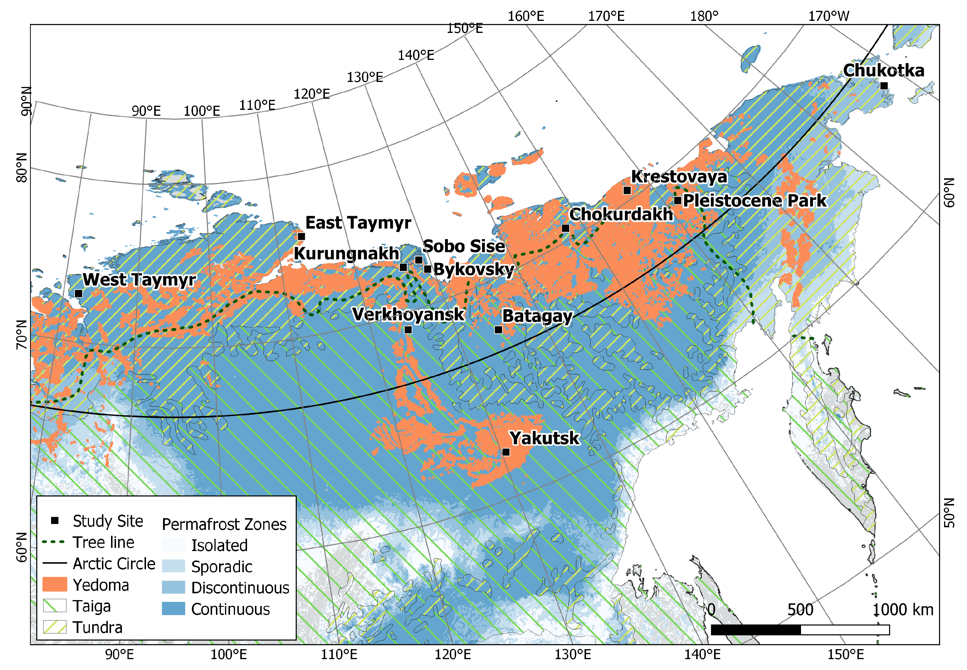
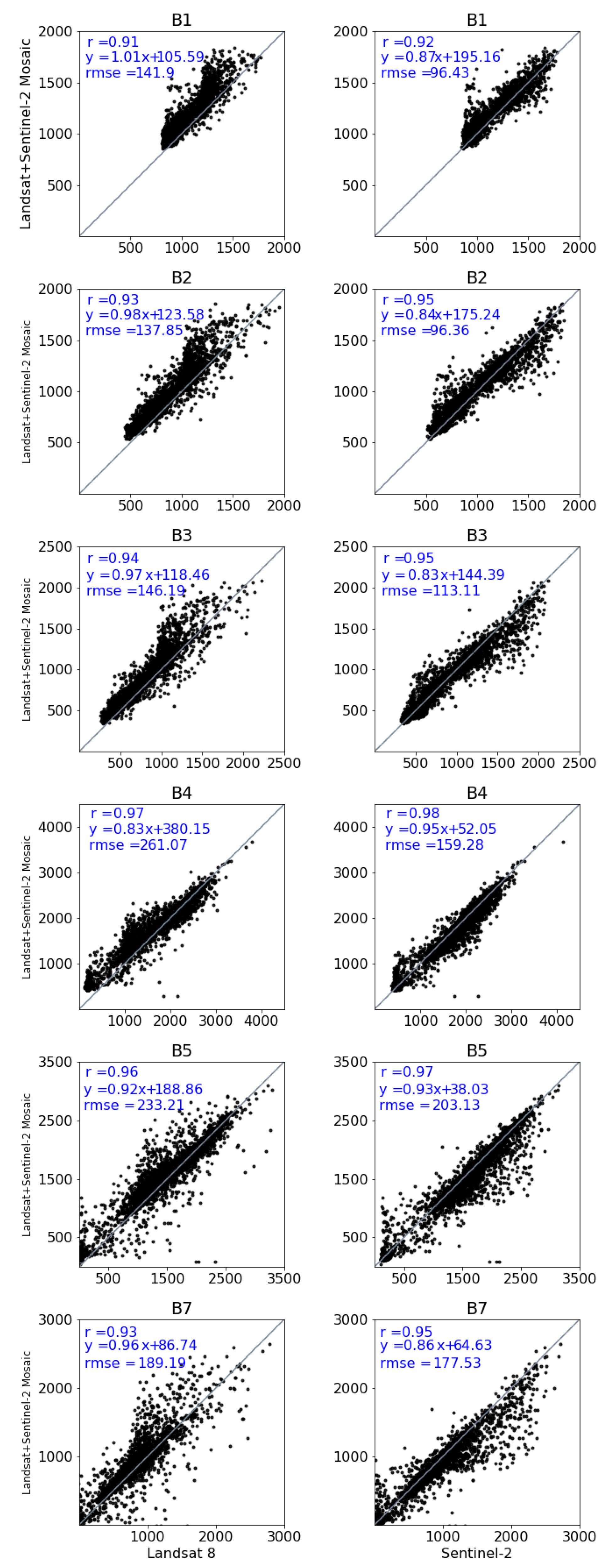
Table 1.
The study sites, their location, and their ecosystem and climatic characteristics.
| Study Site | AOI Coord. [°N, °E] | Ecosystem Characteristics | Climatic Characteristics | MAAT Jan, Jul [°C] | MATP [m] |
|---|---|---|---|---|---|
| Bykovsky | 71.8, 129.3 | coastal, lowland, Yedoma, Tundra | Polar, Moist | −28.2, 3.95 | 0.029 |
| Sobo Sise | 72.5, 128.6 | coastal, lowland, Yedoma, Tundra | Polar, Moist | −32.1, 8.3 | 0.024 |
| Kurungnakh | 72.4, 126.3 | coastal, lowland, Yedoma, Tundra | Polar, Moist | −32.5, 9.97 | 0.024 |
| East Taymyr | 75.6, 113.6 | coastal, lowland, Yedoma, Tundra | Polar, Moist | −28.6, 3.8 | 0.028 |
| West Taymyr | 72.6, 82.0 | coastal, hilly, Tundra | Polar, Moist | −27.1, 8.1 | 0.043 |
| Krestovaya | 70.5, 157.2 | coastal, lowland, Yedoma, Tundra | Polar, Dry | −32.1, 7.7 | 0.020 |
| Chokurdakh | 70.6, 147.9 | coastal, lowland to hilly, Yedoma, Tundra | Polar, Dry | −33.9, 10.2 | 0.024 |
| Pleistocene Park | 68.5, 161.4 | coastal, lowland to hilly, Yedoma, Tundra | Boreal, Dry | −33.1, 13.1 | 0.025 |
| Chukotka | 65.1, −172.1 | coastal, lowland, Tundra | Boreal, Moist | −19.9, 8.97 | 0.052 |
| Batagay | 67.6, 134.8 | inland, hilly to mountainous, Yedoma, Taiga | Boreal, Dry | −41.9, 15.7 | 0.021 |
| Verkhoyansk | 69.1, 124.5 | inland, hilly to mountainous, Yedoma, Taiga | Boreal, Moist | −36.5, 14.9 | 0.032 |
| Yakutsk | 62.1, 130.5 | inland, lowland, Yedoma, Taiga | Boreal, Dry | −38.8, 19.4 | 0.023 |
Table 2.
The cloud-free Landsat and Sentinel-2 images per study site for the spectral band comparison.
Table 2.
The cloud-free Landsat and Sentinel-2 images per study site for the spectral band comparison.
| Study Site | Year | Landsat (LANDSAT/LC08/C01/T1_TOA/) | Sentinel-2 (COPERNICUS/S2/) |
|---|---|---|---|
| Bykovsky | 2018 | LC08_127010_20180826 | 20180727T035541_20180727T035537_T52WEE |
| Sobo Sise | 2018 | LC08_130009_20180815 | 20180828T034529_20180828T034525_T51XXA |
| Kurungnakh | 2018 | LC08_132009_20180728 | 20180809T040541_20180809T040543_T51XXA |
| East Taymyr | 2018 | LC08_204237_20180805 | 20180825T051639_20180825T051642_T49XEE |
| West Taymyr | 2019 | LC08_160009_20190719 | 20190718T064629_20190718T064632_T44XNF |
| Krestovaya | 2016 | LC08_109010_20160806 | 20160804T013657_20160804T032423_T56WPD |
| Chokurdakh | 2018 | LC08_116010_20180813 | 20180804T022549_20180804T022545_T55WEU |
| Pleistocene Park | 2019 | LC08_105012_20190819 | 20190816T012701_20190816T012658_T57WWS |
| Chukotka | 2019 | LC08_085014_20190705 | 20190806T231601_20190806T231556_T02WMT |
| Batagay | 2018 | LC08_122012_20180807 | 20180711T024549_20180711T024544_T53WMR |
| Verkhoyansk | 2018 | LC08_129011_20180808 | 20180808T034529_20180808T034530_T51WWS |
| Yakutsk | 2019 | LC08_120017_20190727 | 20190726T024559_20190726T024554_T52VEP |
Table 3.
Area Coverage Calculation showing the percentage covered of the study sites (AOIarea) by the Landsat mosaic and the combined Landsat+Sentinel-2 mosaic.
Table 3.
Area Coverage Calculation showing the percentage covered of the study sites (AOIarea) by the Landsat mosaic and the combined Landsat+Sentinel-2 mosaic.
| Study Site | Year | Landsat Mosaic [%] | Landsat+Sentinel-2 Mosaic [%] |
|---|---|---|---|
| Kurungnakh | 2016 | 99.7 | 100 |
| 2017 | 69.7 | 100 | |
| 2018 | 100 | 100 | |
| 2019 | 92.2 | 100 | |
| Bykovsky | 2016 | 97.3 | 100 |
| 2017 | 72.9 | 100 | |
| 2019 | 98.7 | 100 | |
| Sobo Sise | 2017 | 27.2 | 100 |
| 2019 | 83.6 | 100 | |
| East Taymyr | 2016 | 97.1 | 99.9 |
| 2017 | 58.1 | 99.9 | |
| Krestovaya | 2019 | 98.5 | 100 |
| Chukotka | 2017 | 95.3 | 100 |
| 2019 | 99.7 | 100 |
Table 4.
The correlation coefficients (r-values) from the spectral band comparisons for each study site between the Landsat image and the Landsat+Sentinel-2 mosaic and between the Sentinel-2 image and the Landsat+Sentinel-2 mosaic (see Table 2).
Table 4.
The correlation coefficients (r-values) from the spectral band comparisons for each study site between the Landsat image and the Landsat+Sentinel-2 mosaic and between the Sentinel-2 image and the Landsat+Sentinel-2 mosaic (see Table 2).
| Landsat 8 | Sentinel-2 | |||||||||||
|---|---|---|---|---|---|---|---|---|---|---|---|---|
| Study Site | B1 | B2 | B3 | B4 | B5 | B7 | B1 | B2 | B3 | B4 | B5 | B7 |
| Bykovsky | 0.82 | 0.87 | 0.85 | 0.99 | 0.99 | 0.99 | 0.75 | 0.88 | 0.89 | 0.99 | 0.99 | 0.99 |
| Sobo Sise | 0.46 | 0.58 | 0.63 | 0.91 | 0.9 | 0.85 | 0.88 | 0.91 | 0.91 | 0.96 | 0.94 | 0.92 |
| Kurungnakh | 0.91 | 0.93 | 0.94 | 0.97 | 0.96 | 0.93 | 0.92 | 0.95 | 0.95 | 0.98 | 0.97 | 0.95 |
| East Taymyr | 0.40 | 0.51 | 0.78 | 0.95 | 0.92 | 0.90 | 0.48 | 0.71 | 0.91 | 0.99 | 0.99 | 0.99 |
| West Taymyr | 0.68 | 0.77 | 0.80 | 0.94 | 0.89 | 0.90 | 0.57 | 0.64 | 0.68 | 0.89 | 0.86 | 0.86 |
| Krestovaya | 0.55 | 0.76 | 0.90 | 0.97 | 0.97 | 0.97 | 0.28 | 0.60 | 0.78 | 0.91 | 0.93 | 0.91 |
| Chokurdakh | 0.61 | 0.78 | 0.85 | 0.98 | 0.98 | 0.96 | 0.61 | 0.79 | 0.84 | 0.97 | 0.97 | 0.95 |
| Pleistocene Park | 0.64 | 0.84 | 0.79 | 0.96 | 0.97 | 0.96 | 0.67 | 0.88 | 0.87 | 0.98 | 0.99 | 0.98 |
| Chukotka | 0.70 | 0.85 | 0.90 | 0.99 | 0.99 | 0.99 | 0.68 | 0.88 | 0.93 | 0.99 | 0.99 | 0.99 |
| Batagay | 0.73 | 0.87 | 0.94 | 0.97 | 0.97 | 0.97 | 0.66 | 0.84 | 0.89 | 0.95 | 0.95 | 0.94 |
| Verkhoyansk | 0.91 | 0.95 | 0.96 | 0.98 | 0.99 | 0.98 | 0.91 | 0.95 | 0.96 | 0.99 | 0.99 | 0.98 |
| Yakutsk | 0.69 | 0.81 | 0.93 | 0.93 | 0.97 | 0.97 | 0.66 | 0.80 | 0.92 | 0.93 | 0.97 | 0.97 |
© 2020 by the authors. Licensee MDPI, Basel, Switzerland. This article is an open access article distributed under the terms and conditions of the Creative Commons Attribution (CC BY) license (http://creativecommons.org/licenses/by/4.0/).
Share and Cite
MDPI and ACS Style
Runge, A.; Grosse, G. Mosaicking Landsat and Sentinel-2 Data to Enhance LandTrendr Time Series Analysis in Northern High Latitude Permafrost Regions. Remote Sens. 2020, 12, 2471. https://doi.org/10.3390/rs12152471
AMA Style
Runge A, Grosse G. Mosaicking Landsat and Sentinel-2 Data to Enhance LandTrendr Time Series Analysis in Northern High Latitude Permafrost Regions. Remote Sensing. 2020; 12(15):2471. https://doi.org/10.3390/rs12152471
Chicago/Turabian StyleRunge, Alexandra, and Guido Grosse. 2020. "Mosaicking Landsat and Sentinel-2 Data to Enhance LandTrendr Time Series Analysis in Northern High Latitude Permafrost Regions" Remote Sensing 12, no. 15: 2471. https://doi.org/10.3390/rs12152471
Note that from the first issue of 2016, this journal uses article numbers instead of page numbers. See further details here.