A New Algorithm for Daily Sea Ice Lead Identification in the Arctic and Antarctic Winter from Thermal-Infrared Satellite Imagery


Department of Environmental Meteorology, University of Trier, 54296 Trier, Germany
*
Author to whom correspondence should be addressed.
Remote Sens. 2020, 12(12), 1957; https://doi.org/10.3390/rs12121957
Submission received: 26 March 2020
/
Revised: 4 June 2020
/
Accepted: 13 June 2020
/
Published: 17 June 2020
(This article belongs to the Special Issue Polar Sea Ice: Detection, Monitoring and Modeling)
Abstract
:The presence of sea ice leads in the sea ice cover represents a key feature in polar regions by controlling the heat exchange between the relatively warm ocean and cold atmosphere due to increased fluxes of turbulent sensible and latent heat. Sea ice leads contribute to the sea ice production and are sources for the formation of dense water which affects the ocean circulation. Atmospheric and ocean models strongly rely on observational data to describe the respective state of the sea ice since numerical models are not able to produce sea ice leads explicitly. For the Arctic, some lead datasets are available, but for the Antarctic, no such data yet exist. Our study presents a new algorithm with which leads are automatically identified in satellite thermal infrared images. A variety of lead metrics is used to distinguish between true leads and detection artefacts with the use of fuzzy logic. We evaluate the outputs and provide pixel-wise uncertainties. Our data yield daily sea ice lead maps at a resolution of 1 km2 for the winter months November– April 2002/03–2018/19 (Arctic) and April–September 2003–2019 (Antarctic), respectively. The long-term average of the lead frequency distributions show distinct features related to bathymetric structures in both hemispheres.
Dataset: 10.1594/PANGAEA.917588
Dataset License: CC-BY
1. Introduction
Sea ice leads are a key feature in the closed pack ice, which represent elongated cracks covering up to hundreds of kilometers in length where open water and thin ice is present. Thereby, they influence the ocean/sea-ice/atmosphere interactions dramatically. Leads are predominantly induced by mechanical stress, namely wind stress and ocean currents [1] and they significantly increase the turbulent heat fluxes between the relatively warm ocean and cold atmosphere during wintertime [2,3]. Sea ice leads influence the lower atmosphere by reducing the overall sea ice concentration and thereby warming the regional atmospheric boundary layer [4,5]. In an idealized model study, Reference [6] show that small decreases in the sea ice fraction by 1% at ice concentrations larger than 90% cause a rise of the near-surface temperature by up to 3.5 K. According to Reference [7], the heat flux at constant sea ice concentration is increased when multiple leads are present compared to a single and equal area of open water. Because of the associated ocean heat loss in leads, new sea ice is produced, causing significant salt rejection, which in turn affects dense water formation and the ocean circulation [1,8,9,10].
Ice-free areas including sea ice leads were also identified as sources for methane emissions [11,12]. The relevance of leads, polynyas and the sea ice edge for marine species is shown in Reference [13]. Weather prediction, climate, and ocean models rely strongly on detailed information on the respective state of the sea ice. The majority of numerical models, however, cannot produce sea ice leads explicitly and sea ice concentrations from passive microwave data are too coarse to resolve leads [14,15].
Thus there is a need to develop and provide new algorithms to retrieve daily maps of sea ice leads on circum-polar scales in both hemispheres. So far, no dataset exists which describes a climatology of the daily distribution of sea ice leads in both polar regions in a consistent way. Almost all of the previously published studies are conducted for the Arctic and focus on smaller regions and time scales or have coarser geometric resolutions.
The potential of thermal infrared satellite data for the detection of sea ice leads is shown in References [8,16]. However, lead detections then there rely on clear-sky situations and on winter months only to make use of a high temperature contrast between open water and sea ice. Leads in the Arctic are manually identified based on thermal imagery in Reference [17] with a 5-year climatology of wintertime leads derived for the years of 1979/1980 to 1984/1985. Data from the Moderate-Resolution Imaging Spectroradiometer (MODIS) are used in References [18,19] to derive maps of potential open water per pixel and they furthermore evaluate the potential of this approach as a sea ice concentration retrieval method. The differentiation between thick and thin sea ice, including polynyas and leads, was successfully demonstrated in Reference [20], where a polarization ratio of two frequencies of the Advanced Microwave Scanning Radiometer-EOS (AMSR-E) was used. Due to the footprint of the sensor, they identify only leads broader than 3 km and produce daily wintertime lead maps for the Arctic for the winters 2002–2012. The follow-up study from Reference [21] presents a 9-year lead climatology in the Arctic Ocean, revealing multiple hot spots with increased lead observations in the Beaufort Gyre and close to the Fram Strait.
Leads in the Arctic are identified in SAR images from CryoSat-2 and lead fractions and lead width distributions are derived by optimizing the threshold applied on the backscattered waveforms [22]. However, data are presented only for the winters 2011 and 2013 and the derived sea ice products have a comparably low spatial resolution of around 100 km × 100 km. Another approach uses thermal imagery from MODIS, where sea ice leads are identified based on their positive surface temperature anomaly [23]. The authors produce daily maps of sea ice leads with a spatial resolution of 1.5 km × 1.5 km for the months of January to April in the Arctic from 2002 to 2015 [24]. Remaining cloud artefacts that usually represented an obstacle for an automatic lead detection are removed with a fuzzy inference system.
The available lead fractions from AMSR-E [20] are evaluated in Reference [25] by using lead observations in SAR data as a reference, and show that AMSR-E overestimates the lead fraction compared to the SAR data, particularly the lead fraction classes near 100%. A further lead retrieval algorithm for CryoSat-2 data was developed by Reference [26] making use of the specific waveform of the backscattered signal to identify leads as in Reference [22]. They present monthly averages for lead fractions in the Arctic on a 10 km grid covering the years 2011 to 2016 and compare their results with the products from Reference [20] (AMSR-E), Reference [23] (MODIS), and Reference [22] (CryoSat-2) for the respective period. They reveal differences in the data sets due to differences in the spatial and temporal resolution of the used satellite sensors. A study by Reference [27] uses MODIS thermal infrared data with an approach similar to References [23,24] using a fixed threshold and a sequence of multiple tests to produce daily Arctic lead maps.
Since no lead fraction data set exists at this time for the Antarctic, this study aims at presenting a new and robust lead retrieval algorithm that is applicable in both polar regions. Furthermore, we present long-term average lead frequencies for wintertime sea ice in the Arctic (November–April 2002/03–2018/19) and the Southern Ocean (April–September 2003–2019). The algorithm expands upon the work of Reference [23], including major improvements and an adaption to the Southern Hemisphere. Therefore, not only a new lead dataset for the Antarctic is obtained, but also the existing lead dataset for the Arctic [24] receives an extension and update. We use satellite thermal infrared data from MODIS to derive daily maps of leads for the winter months, that is, November to April for Arctic sea ice and April to September for Antarctic sea ice, respectively, including pixel-based retrieval uncertainties. In Section 2, we present the used data and applied methods in detail, which comprise the tile-based processing, the fuzzy filtering and manual quality control for both hemispheres. In Section 3, we show example results of the new lead retrieval approach and go ahead with a discussion of the implemented methods, showing strengths and potential shortcomings of the algorithm in Section 4.
2. Data and Methods
We use collection 6 of MYD/MOD29 ice surface temperature (IST) data [28] to infer daily sea ice leads for both polar regions. MODIS, onboard the two satellites Terra and Aqua (NASA-EOS), provides data since 2000 (Terra) and 2002 (Aqua) and acquisitions are stored in 5-min tiles with a 1 km spatial resolution at nadir. The product includes the MODIS land and cloud mask. An overview of the most important information on both polar regions is presented in Table 1. The cloud fraction for sea ice areas in both hemispheres is defined as the long-term average of daily cloud fractions. The cloud fraction is derived from the MODIS cloud mask and represents the fraction of cloud observations in relation to the maximum number of tiles per pixel.
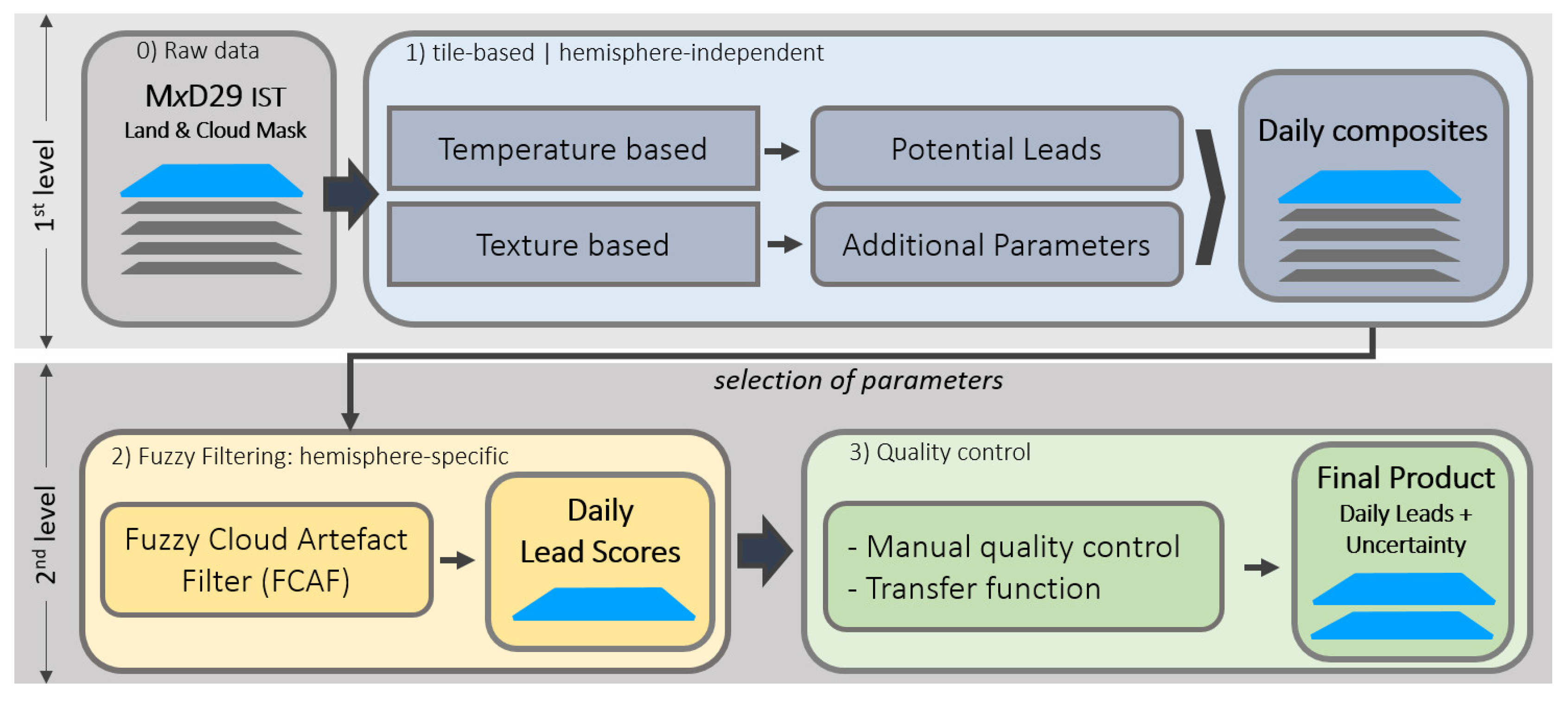
Due to the open water or thin ice present in leads, these can be identified as a warm temperature anomaly, surrounded by cold sea ice. Although the MODIS cloud mask is applied to select clear-sky pixels, the satellite image may be partially covered by clouds or fog that is not included in the mask. A significant fraction of unidentified clouds appear as warm features, which are consequently misinterpreted as leads by unsupervised algorithms. Therefore, a two-stage processing chain is applied, consisting of (1) lead detection, where potential leads are retrieved from the IST data and (2) filtering, where a fuzzy filter is applied to remove false detections. An overview of the processing is provided in Figure 1.
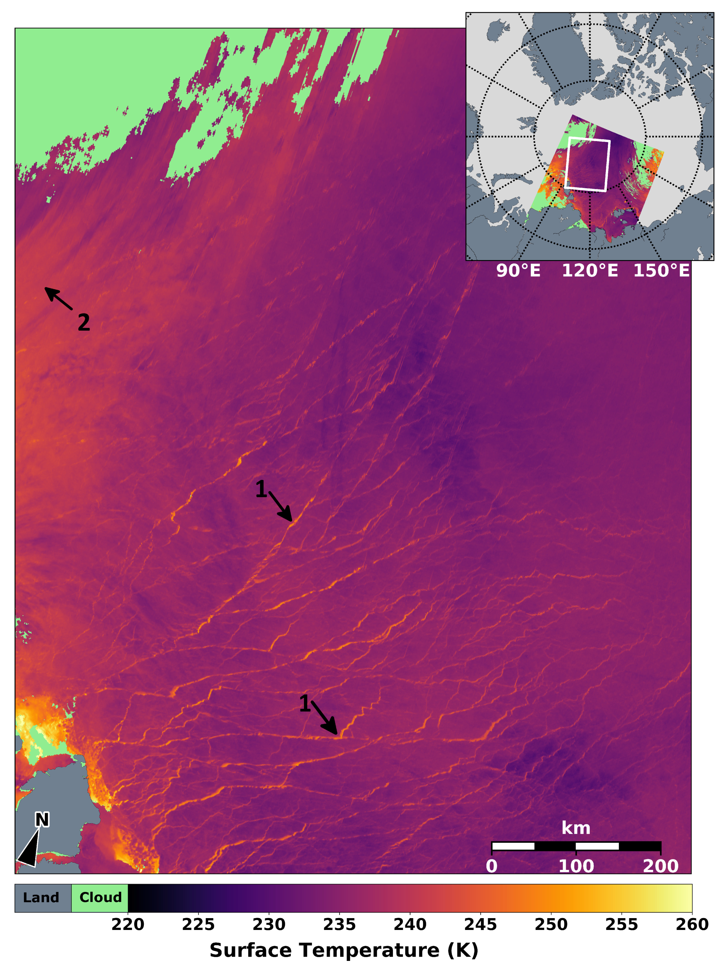
The tile displayed in Figure 2 shows the IST from the MYD29 product (Aqua) for a region in the central Arctic on January 21, 2008. The presented data type corresponds to the 0-th processing step (raw data) in Figure 1. The warm signature of sea ice leads is clearly visible (arrow 1). The MODIS land and cloud mask are also shown. Undetected clouds are visible in the satellite image and can appear as warm features (arrow 2) and represent the major source of errors and noise in automatically derived lead maps. For the preparation of daily maps we make use of multiple daily satellite overpasses and an associated stacking to fill data gaps that result from the MODIS cloud mask.
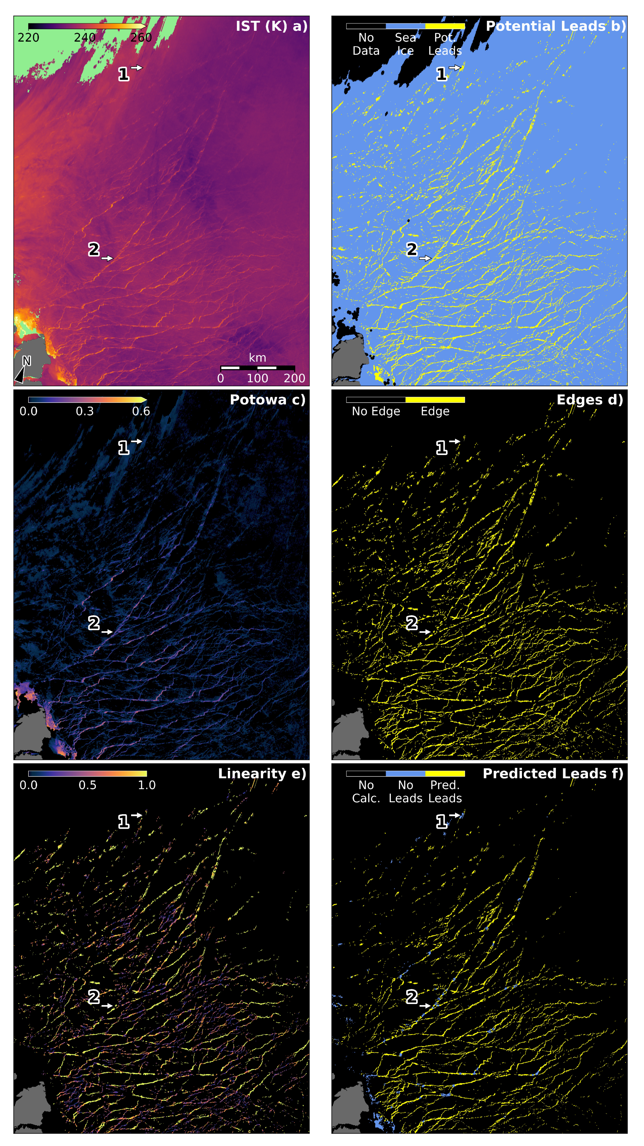
First, potential leads are identified from the local surface temperature anomalies. To support the subsequent filtering, additional metrics are derived. This step is identical for both the Northern and Southern Hemispheres (Figure 1, box 1). A selection of derived parameters is provided in Figure 3, where the IST is shown as reference (Figure 3a). Based on the IST, local thresholding with a 51 × 51 kernel is applied on the tiles to identify pixels that are significantly warmer than the local neighborhood (Figure 3a, arrow 2). By this, large-scale temperature gradients due to different air masses are omitted while the relative surface temperature contrast is preserved. From this, we obtain potential leads (Figure 3b). This parameter also includes other warm temperature anomalies, which are not associated to sea ice leads, namely cloud artefacts (top arrow 1). Therefore, we derive a set of additional metrics that will allow for a better differentiation between true leads and artefacts. The potential open water POTOWA is based on the IST and describes the fraction of a pixel covered by open water [16,18], which is the inverse of sea-ice concentration (Figure 3c). This concept assumes that a pixel is composed of a mixture of different surface types, namely open water and sea ice. For leads (arrow 2), the POTOWA values are higher than in the surrounding. Warm features arising from clouds, for example arrow 1, have low to medium POTOWA values. By applying a Canny filter [29] on the POTOWA, strong gradients are detected, which are indicative of sea ice lead edges (Figure 3d). By this, most of the features with low to medium POTOWA are excluded.
We derive additionally a linearity measure of potential lead objects by calculating two-dimensional angular variability similar to a Hough transform (Figure 3e). Consequently, leads have the highest linearity values combined with medium to high POTOWA (arrow 2), while cloud artefacts are characterized by low linearity scores combined with low to medium POTOWA (arrow 1). We furthermore derive a predicted lead indicator for every pixel based on different input parameters, for example, the linearity, Canny edges, and other texture parameters derived from gray-level co-occurrence analysis namely the dissimilarity, homogeneity, and correlation (Figure 3f). For this purpose, a universal logistic regression model is set up and trained with manually classified IST tiles. The output of the logistic regression is binary, where 1 (yellow pixels) represents predicted true leads. Here, cloud artefacts (arrow 1, Figure 3f) are classified as ‘no leads’.
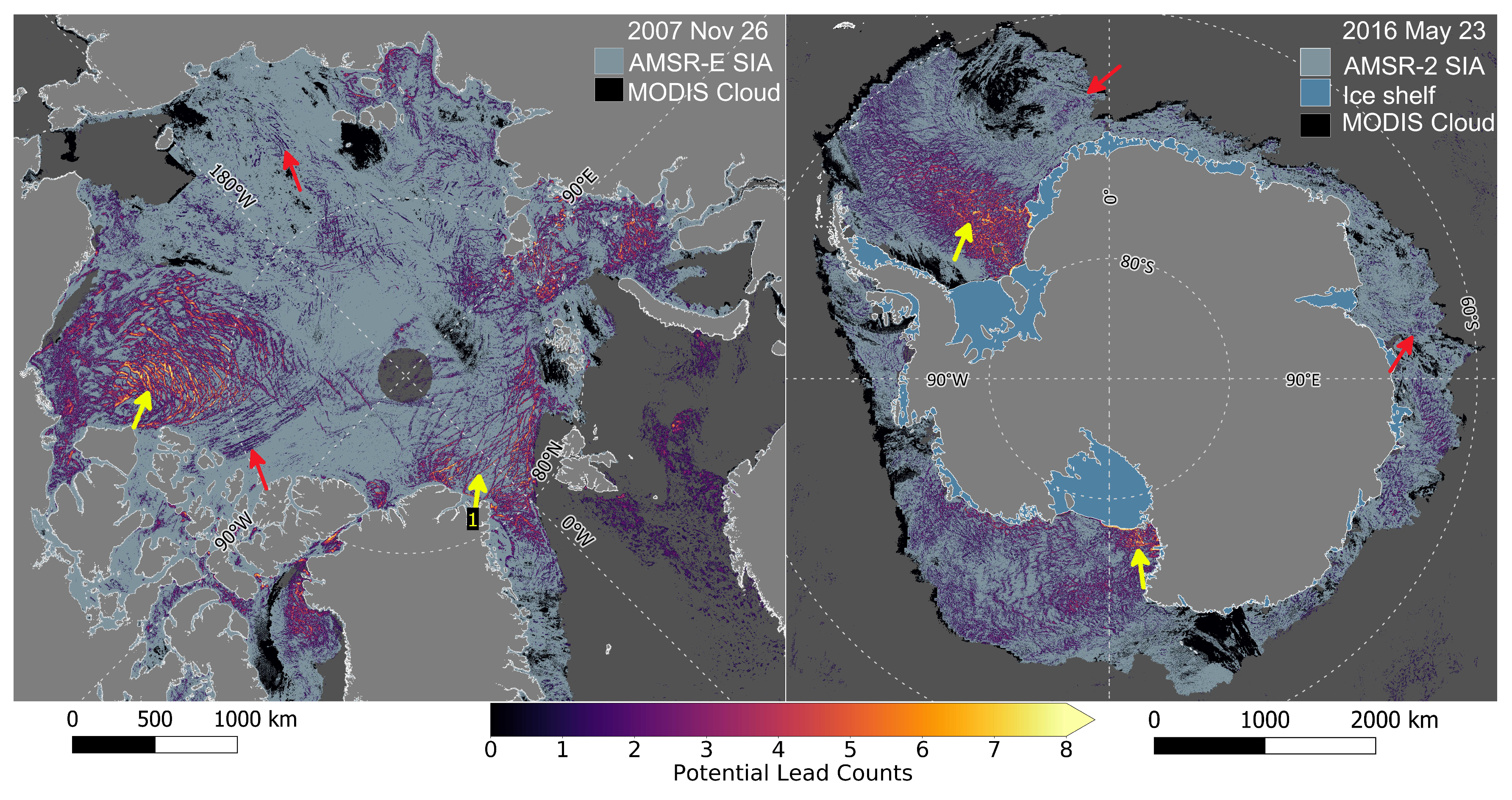
After all parameters are derived, the tiles are combined to daily stacks by reprojecting them to the respective reference grid (ARC: EPSG:3413, ANT: EPSG:3412) by calculating the sum or average for the respective parameter (see also Figure 1 box 1c). As an example for one of the obtained daily stacks, Figure 4 shows the potential lead count as the daily sum of potential lead detections for the Arctic (left, 26 November 2007) and the Antarctic (right, 23 May 2018), with the sea ice cover (>15% concentration) derived from AMSR-E/AMSR-2 in the background (blue). Areas that were permanently covered by clouds during the respective day are colored black. The potential lead count indicates the presence of leads, where the maximum value varies around 12 daily observations, depending on the number of tiles per day and on the cloud coverage during a day. High values show rather persistent lead objects (yellow arrows), while lower values indicate the presence of less frequently identified leads or artefacts (red arrows), that is, remaining warm cloud features that fulfilled the criteria of being identified as a potential lead. Due to the faster movement of clouds compared to the sea ice cover, a false lead detection from cloud artefacts generally receives low counts. Some real leads may receive low counts (e.g., yellow arrow 1 in the Fram Strait) due to clouds, which reduce the total number of observations per day, or due to closing of the leads during the day because of changes in the sea ice drift, which makes the count parameter by itself insufficient to separate leads from artefacts. For this reason, we prepare additional daily stacks from the metrics that are described above, for example, linearity and texture parameters. For the day shown in Figure 4, sea ice leads indicated by yellow arrows are mainly visible in the Beaufort Gyre and the Fram Strait (left, Arctic) and in the Antarctic in the southeastern Weddell Sea and Ross Sea (right, Antarctic).
To further differentiate between true leads and warm temperature artefacts, we use an extended version of the fuzzy filter introduced by Reference [23] and use two different set ups for each hemisphere. With fuzzy logic a multi-layer input data set can be processed and translated into a combined, single-layer result by using a set of membership functions and rules [30]. The great advantage over black-box algorithms where the transfer functions are not directly accessible (e.g., neural networks, clustering algorithms) is that the user is able to modify the system by selecting specific membership functions and rules. The defined rules are of linguistic format, hence they can be interpreted easily and expert knowledge can be included in a straightforward manner. The output data is continuous and determines the degree to which a certain pixel belongs to the output membership, hereafter called Lead Score (LS). It can be understood as an indirect measure of uncertainty and is re-calculated into uncertainty by conducting a manual quality control in the subsequent processing step. The selection of input parameters, definition of membership functions and rules involves user knowledge and has the aim to maximize both the true positive classification of sea ice leads and the obtained LS range. In the following we refer to this filtering as the Fuzzy Cloud Artefact Filter (FCAF). For further processing, we defined two different FCAFs to compensate for hemisphere-specific requirements, which are mainly caused by the different spatial coverage and mobility of the sea ice extent. In the Antarctic, sea ice extends further north, and is therefore more frequently influenced by warm air advection from mid-latitudes. Associated to the warm air advection are clouds, which is shown by the higher average cloud fraction compared to the Arctic (Table 1). The temperature contrast is also reduced when warm air is advected, thus increasing the uncertainty for the identification of leads based on their temperature anomaly. The input parameters for the FCAFs for the Northern and Southern Hemispheres are listed in Table 2. Two additional parameters are calculated for the FCAF, namely the background temperature anomaly and the clear sky ratio. The first represents the daily averaged regional surface temperature minus its climatological mean. It turns out, that large-scale positive surface temperature anomalies are particularly associated with the formation of clouds and reduce the IST contrast over leads, making the background temperature anomaly a valuable additional metric for the FCAF. The clear sky ratio is the fraction of clear-sky observations per day in relation to the maximum possible number of observations, that is, number of tiles per day and pixel and represents a useful metric to address confidence to a lead retrieval.
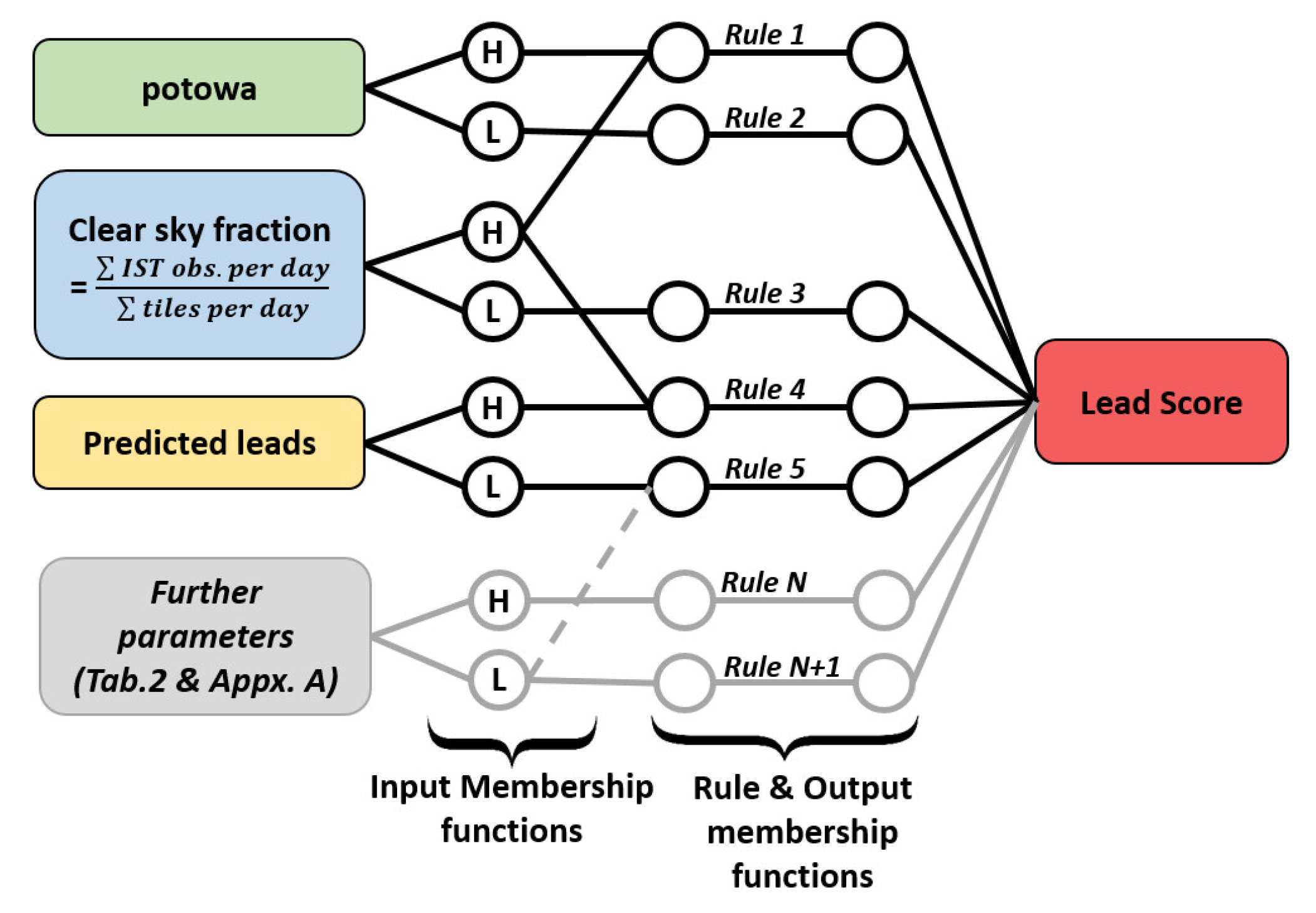
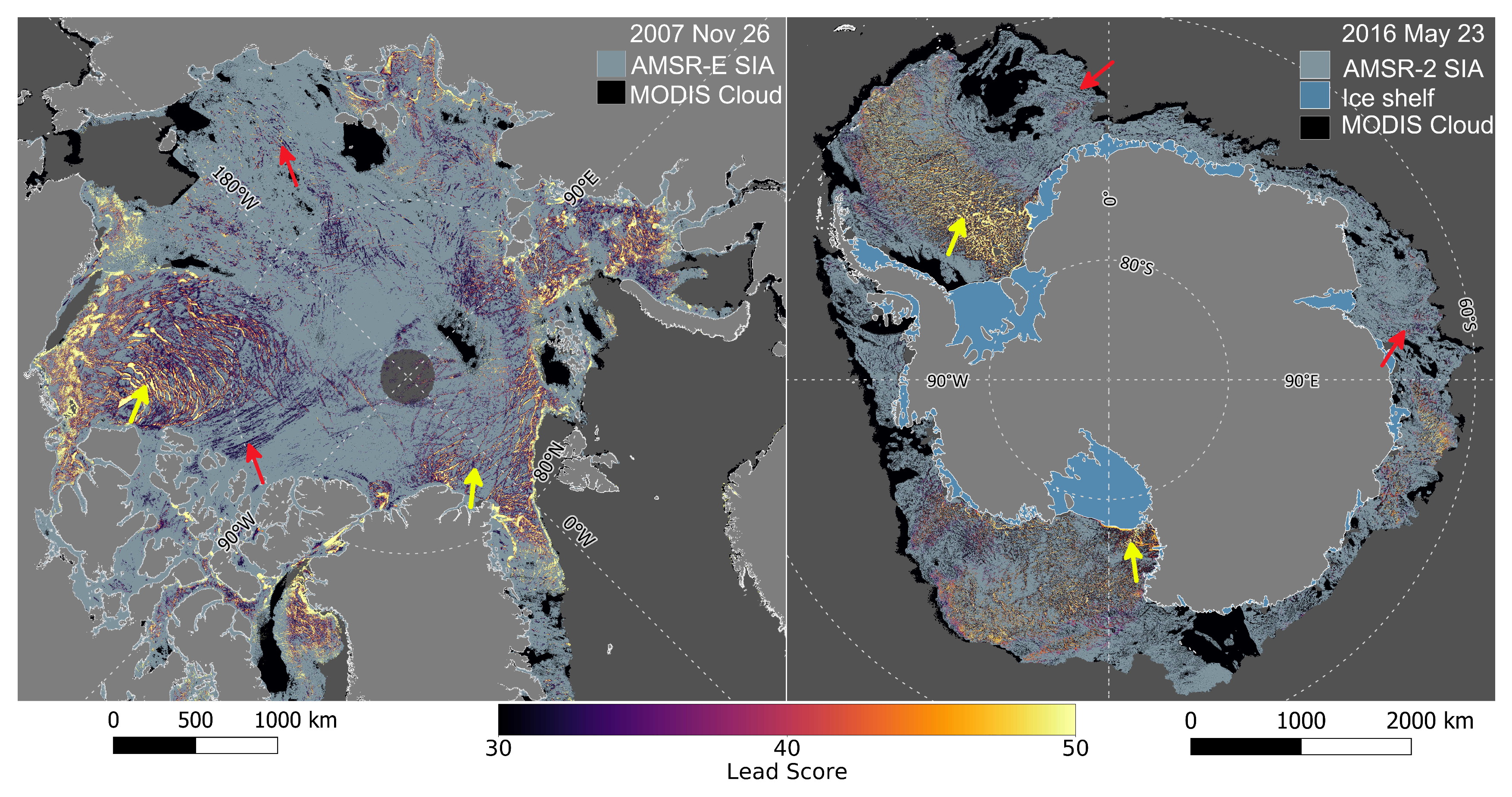
In Figure 5 an outline of the FCAF is shown, indicating that all input parameters are combined by internal fuzzy variables and membership functions, processed accordingly and the final LS is thereby calculated for every day. For instance, the POTOWA is combined with the clear sky ratio by formulating the rule, that both must have high values for the LS to be high. An overview of the fuzzy rules for both polar regions is given in Table A1, respectively. An example of the retrieved daily LS maps for the Arctic and Antarctic is presented in Figure 6. As indicated by yellow arrows, high LS values are present in the Beaufort Gyre and Fram Strait (left, Arctic), or in the Weddell Sea and Ross Sea (right, Antarctic) and indicate the presence of sea ice leads with high confidence. Red arrows, however, are rather indicative of lead detection with lower confidence or artefacts.
3. Results
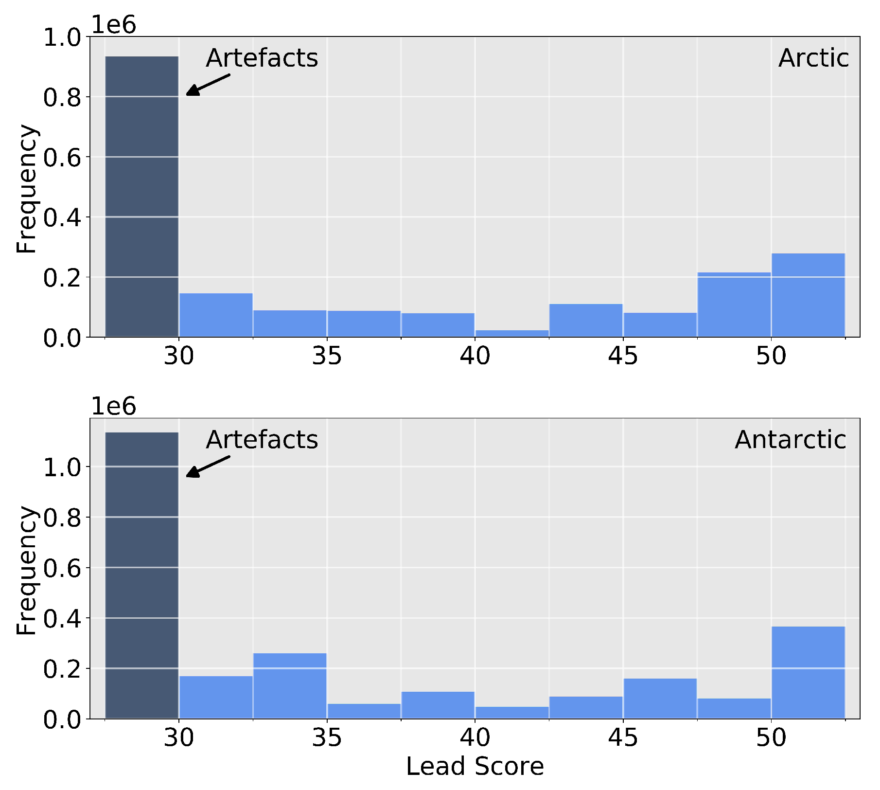
The LS histograms for both hemispheres are presented in Figure 7. Both distributions show a large mode of LS values smaller than 30 and lower but increasing frequencies for higher LS values. The large class of LS values below 30 contains pixels that are prone to a low probability for a true lead, which emerges from the fuzzy rules and emberships applied. However, true leads may be included in the artefact class but with a high retrieval uncertainty. In contrast, the LS exceeding a value of 30 provides increasing confidence for the presence of a true lead. The LS is not a direct measure for uncertainty, but rather an indicator that a respective pixel belongs gradually to either artefacts or leads. Therefore, we performed a manual quality control to associate LS values with the probability of false detections and to derive the associated transfer function, with which we can then obtain pixel-wise uncertainties.
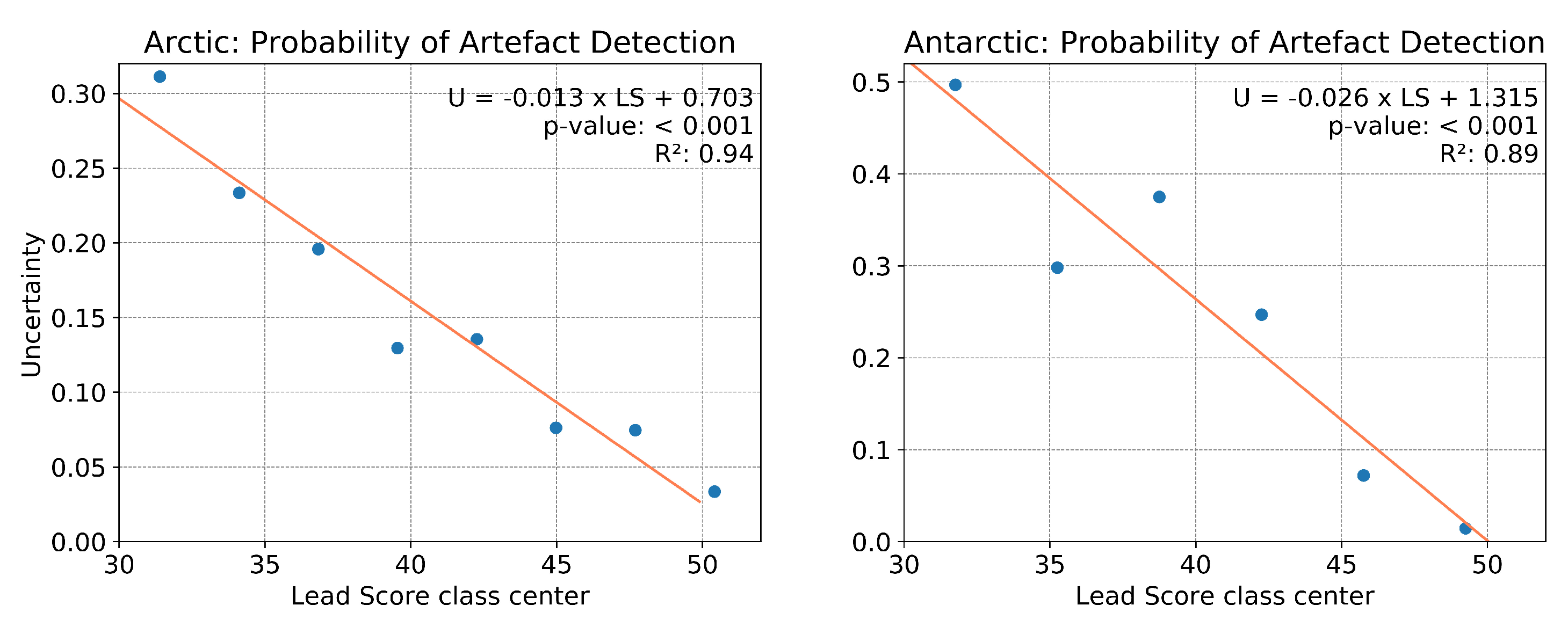
We conduct a manual quality control (MQC) for each hemisphere yielding two different transfer functions for the calculation of detection uncertainty from LS. Within a set of 6 representative LS maps for each hemisphere, areas containing true sea ice leads and artefacts were visually identified and classified, respectively. Subsequently, the probability of artefact detection is calculated for each of the applied LS classes. Afterwards, a linear regression model describing the relation between probability of artefact detection and LS class yields the transfer function, which is used to calculate pixel-wise uncertainties (Figure 8). The previously identified artefact class (LS < 30) is not included in the linear regression, but obviously corresponds to uncertainties larger than 30% (Arctic) and 50% (Antarctic). The slope of the transfer function for the Arctic is smaller compared to the Antarctic, indicating that the uncertainty is higher for most areas in the Antarctic. However, for LS larger than 45 the uncertainty decreases to less than 10% in both hemispheres.
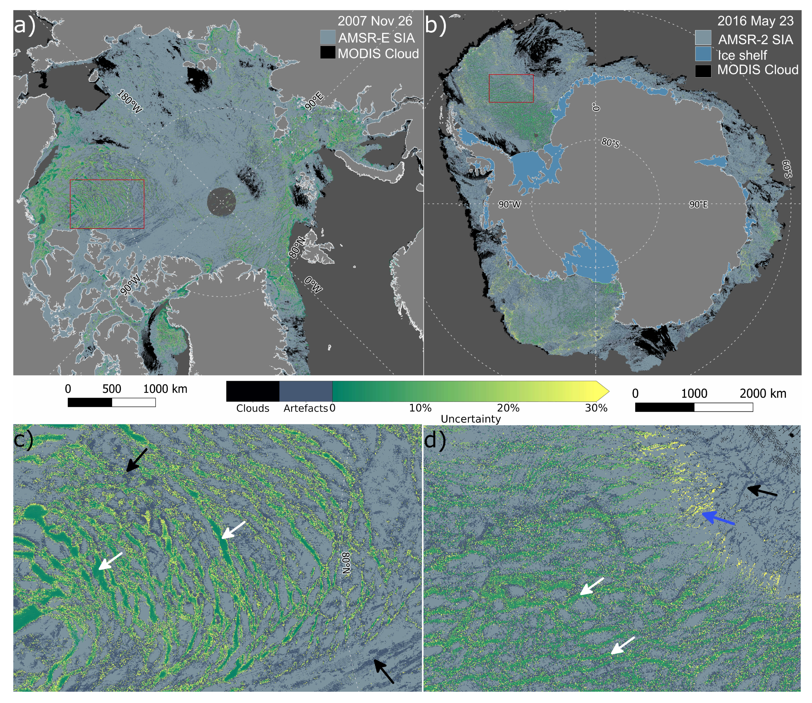
Figure 9 shows the resulting lead uncertainties for the Arctic and Antarctic for one day with a detailed view corresponding to the red rectangle. White arrows indicate the location of identified leads with low uncertainties, while dark-gray colored areas correspond to artefacts and black colored areas represent the MODIS cloudmask. The artefact class can be used as an additional cloud mask, meaning that no information about surface features is available. For the presented day in the Arctic, leads with high confidence can be seen throughout the entire hemisphere with pronounced leads in the Beaufort Gyre, Fram Strait, Baffin Bay, and Kara Sea. In the Antarctic, leads are predominantly present in the Weddell Sea and in the Ross Sea. The influence of clouds and large-scale temperature gradients is visible in the smooth gradient of uncertainties indicated by the blue arrow (Figure 9d). The uncertainty increases in the neighborhood of clouds due to the associated warm air advection in this case, which in turn evokes a positive temperature anomaly weakening the local temperature contrast.
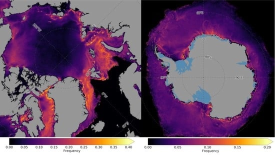
Based on the obtained daily lead data we can derive long-term average lead frequencies for both hemispheres. Figure 10 shows the relative lead frequency for the Arctic (2002/03 to 2018/19, November to April) and the Antarctic (2003 to 2019, April to September) as derived from the daily lead observations. For this purpose, all daily lead maps were averaged over the respective time-period, with artefacts (LS < 30) being excluded. For both hemispheres, increased lead frequencies can be seen along the shelf break. In the Arctic, lead frequencies are also increased in the Beaufort Gyre, Baffin Bay, the Greenland, and the Barents Seas. Similarly, patterns of increased lead frequencies are present in the Antarctic, where for instance north of the coastline a band of increased lead frequencies is visible. Additionally, lead frequencies increase where islands and deep sea features in the bathymetry are present, that is, ridges and troughs. Thereby, frequencies exceed 0.4 (Arctic) and 0.2 (Antarctic) in several regions.
Based on the presented algorithm, a data set for both hemispheres was produced which includes daily fields of sea ice leads and the pixel-wise lead retrieval uncertainty. The lead data contains the classes of sea ice, leads, artefacts, cloudmask, landmask, and areas of open water.
4. Discussion
In the presented algorithm, we consider leads as pixels with a significant local temperature anomaly, which suggests that the fluxes of latent and sensible heat are enhanced at identified leads [2,3]. Leads also contribute to the formation of dense water due to the production of new ice and the associated brine rejection, which ultimately affects the ocean circulation [1,8,9,10]. The mentioned processes associated to leads imply that our results represent a data set, which can be used for for example, high-resolution modelling studies. Although the spatial resolution was increased compared to the product of References [23,27], further research needs to be done to derive leads with higher spatial resolution on a circum-polar scale, since References [6,7] show that particularly narrow leads effectively contribute to these exchange processes.
However, our presented algorithm allows the first comparable observation of sea ice leads in both hemispheres. The definition of leads is consistent in both hemispheres and allows a better inter-hemispheric comparison. To increase the quality of our results, we derive temperature-, shape- and texture-based metrics, for example, the linearity as an indicator for sea ice leads. In doing so, we include a number of independent metrics, which all are solely based on IST data and are subsequently used to separate artefacts from true leads. A major improvement—compared to the previous study by Reference [23] and other studies using fixed thresholds, for example, References [16,27]—is the use of an adaptive local thresholding technique which ensures the identification of potential sea ice leads, particularly when the local temperature contrast is weak due to warm air advection. Consequently, more potential sea ice leads are identified. However, we only make use of clear-sky situations and constrain our lead detection to the winter months to benefit from a generally high temperature contrast between open water and sea ice.
Because of the sea ice drift, leads might be relocated during the course of one day. Our procedure aims to provide data from which one can infer where a lead, that is, a significant local surface temperature anomaly, was identified during the course of one day, regardless of the drift. In the final data product, a strong drift induces an increase in uncertainty to the margins of a lead due to a decreased number of daily lead observations per pixel. Since the ice motion is in some areas on the order of approximately 10 km/d ([31,32], narrow leads in regions of strong ice drift are affected the most by this circumstance. The advantage of our approach including pixel-based uncertainties is, in this regard, that we do not have to make a decision on whether to include observations of drifting leads to the daily map or not, but rather to assign an individual uncertainty value to single lead identifications, which will in turn address the local impact of the respective lead on exchange processes.
To compensate for cloud artefacts, we apply the FCAF that was successfully used in Reference [23] and use different input data and apply specific rules for each hemisphere, respectively (Table 2) to ensure a high data quality. Since the largest source for errors is unidentified clouds, the FCAF is designed to recognize cloud artefacts. Rather than assessing the identified lead objects by a chain of several tests (Bulk lead detection in Reference [27]), we apply the FCAF to assess the derived metrics with respect to true leads and cloud artefacts simultaneously. We support our derived lead maps with pixel-wise uncertainties which can be used as a quality flag. The above mentioned sea ice drift and displacement of sea ice leads as well as large-scale warm air advection result in an increased uncertainty of a detected lead. However, the pixels in the core of a lead as well as slow moving leads receive lower uncertainties and thereby provide higher confidences. The resulting artefact class might be used as an extension for the MODIS cloud mask. With respect to the inter-hemispheric comparison of lead retrieval uncertainties, Figure 8 indicates that uncertainties for the Antarctic are generally higher than for the Arctic, which is caused by a generally higher cloud fraction (Table 1) and a smaller repetition rate of satellite overpasses due to the geographical extent. This results in less frequent clear-sky observations. However, uncertainties also drop below 10% for the highest LS classes, indicating that it is possible to detect leads with high confidence but at the cost of loosing more true leads to the artefact class.
As mentioned in, for example, Reference [16] the observed leads depend highly on the data used. For surface temperature data where the local temperature contrast between leads and the surrounding sea ice is crucial, differences to other retrieval algorithms using passive or active microwave data, for example, AMSR-E or SAR, (e.g., References [20,22]) can be expected not only because of the spatial resolution but also because of the satellite sensor specification and acquisition mode. Reference [20] rely on passive microwave data and identify leads broader than 3 km, which results in less lead observations compared to our results. Also the broadly used SIC data from passive microwave data are not capable of resolving smaller leads as it is demonstrated for the Arctic in Reference [23]. Although we use multiple overpasses by the satellite sensors to fill data gaps, some areas are persistently covered by clouds throughout a day, which means that data gaps remain in the daily lead maps. A multi-day average or merging with other data products, for example, Reference [20], might be a valuable approach to fill remaining data gaps.
Several hot spots where sea ice leads are predominantly present can be identified, for example, the Beaufort Gyre, Greenland Sea, and Barents Sea (Arctic) and the Weddell Sea and Ross Sea (Antarctic). Similar to the studies by Reference [24] for the Arctic and Reference [33] for the Antarctic, we calculated the long-term average lead frequency based on the filtered data (Figure 10), which reveals persistent lead locations in both hemispheres with respect to lead occurrences, where frequencies of 0.4 (Arctic) and 0.2 (Antarctic) are exceeded in several regions, for example, along the continental shelf break and bathymetric features in the deep sea. Compared with the long-term average of potential leads in the Antarctic as shown in Reference [33] (Figure 1), the filtered lead frequencies are lower due to the application of the FCAF, which removes artefacts from the potential lead maps. However, the overall pattern with increased frequencies along the shelf break as well as over troughs and ridges are preserved after the filtering.
The derived daily lead maps can be used for different applications. First, we consider them as a useful boundary field for regional climate and ocean modeling. Especially with the provided uncertainty, an assimilation of daily lead maps becomes feasible. Second, the lead maps can be interpreted in comparison to other lead products (e.g., References [15,26]) and third, the lead data can be used to analyze temporal and spatial patterns in lead characteristics and potential forcings in both hemispheres.
5. Conclusions and Outlook
This study presents a new and robust algorithm to produce daily maps of sea ice leads for the Arctic (November to April) and Antarctic (April – September). Based on thermal satellite imagery from MODIS, we first process all individual swaths and identify potential sea ice leads and further metrics, and second remove cloud artefacts emerging from deficits in the MODIS cloud mask with the FCAF. Finally, we conduct a manual quality control and calculate pixel-wise uncertainties and obtain daily circum-polar maps of sea ice leads. With the developed algorithm, we present an update for the Arctic and introduce a new lead data set for the Antarctic and present maps of the long-term average lead frequencies for both hemispheres.
The pixel-wise uncertainty will allow for an assimilation of the presented lead maps into boundary conditions for regional climate models and thereby support improved heat flux calculations. In the follow-up studies, we plan to study the spatial and temporal dynamics of sea ice leads for both hemispheres in detail. By doing so, we aim to reveal the long-term evolution of sea ice leads in both hemispheres with respect to atmospheric and oceanographic forcings. The comparison of our produced lead data with others is also planned and will help to improve our understanding of the small scale sea ice dynamics.
Author Contributions
Conceptualization, F.R., S.W.; Methodology, F.R., S.W., G.H.; Software, F.R., S.W.; Formal Analysis, F.R., S.W.; Data Curation, F.R., S.W.; Writing—Original Draft Preparation, F.R.; Writing—Review and Editing, F.R., S.W., G.H.; Visualization, F.R.; Supervision, S.W., G.H.; Project Administration, G.H.; Funding Acquisition, G.H., S.W. All authors have read and agreed to the published version of the manuscript.
Funding
The research was funded by the Deutsche Forschungsgemeinschaft (DFG) in the framework of the priority program “Antarctic Research with comparative investigations in Arctic ice areas” under Grants HE 2740/22 and WI 3314/3 and it was also supported by the Federal Ministry of Education and Research (BMBF) under grants 03F0776D and 03F831C. The publication was funded by the Open Access Fund of the University of Trier and the German Research Foundation (DFG) within the Open Access Publishing funding program.
Acknowledgments
The authors want to thank the NSIDC for providing the MODIS IST data. All processing was done in Python3. We also want to thank J.D. Warner for the implementation and his support during the usage of the fuzzy logic in python (scikit-fuzzy) and we acknowledge the Norwegian Polar Institute’s Quantarctica package version 3 and the QGIS Development Team. The supplementary data (lead climatology for the Arctic and Antarctic) are available at the online archive PANGAEA (https://doi.org/10.1594/PANGAEA.917588).
Conflicts of Interest
The authors declare no conflict of interest.
Abbreviations
The following abbreviations are used in this manuscript:
| AMSR-E | Advanced microwave sensor EOS |
| EOS | Earth Observing Satellite |
| FCAF | Fuzzy Cloud Artefact Filter |
| IST | Ice surface temperature |
| LS | Lead Score |
| MODIS | Moderate resolution imaging spectroradiometer |
| MQC | Manual quality control |
| SAR | Synthetic Aperture Radar |
Appendix A
As described in Section 2, we use two FCAFs for each polar region. In Figure 5 and Table 2 the relevant input data and a schematic illustration of the fuzzy membership functions and rules are shown. Table A1 present additional information about the hemisphere-specific input data and the corresponding fuzzy membership functions and rules for the Arctic (top) and the Antarctic (bottom). For the respective rules, where multiple input data are included, they are combined with the operation and. All weights for the rules are the same.

Table A1.
Fuzzy rules for the Arctic (top) and the Antarctic (bottom) with high input variables corresponding to high LS (left column) and low input variables corresponding to low LS (right column). Multiple input variables for one rule are combined by the operation and. The parameters are described in Table 2 in Section 2.
| input ’high’ → LS ’high’ | input ’low’ → LS ’low’ | |
|---|---|---|
| ARCTIC | potential leads | potential leads |
| predicted leads | ||
| edges | ||
| combined texture | ||
| POTOWA | ||
| backgr.t-anomaly | ||
| clear sky ratio | ||
| ANTARCTIC | potential leads | potential leads |
| predicted leads | ||
| clear sky ratio | clear sky ratio | |
| linearity | ||
| combined texture | ||
| white tophat POTOWA | ||
| backgr. t-anomaly |
References
- Smith, S.D.; Muench, R.D.; Pease, C.H. Polynyas and leads: An overview of physical processes and environment. J. Geophys. Res. 1990, 95, 9461–9479. [Google Scholar] [CrossRef]
- Alam, A.; Curry, J. Lead-induced atmospheric circulations. J. Geophys. Res. 1995, 100, 4643–4651. [Google Scholar] [CrossRef]
- Maykut, G.A. Energy exchange over young sea ice in the central Arctic. J. Geophys. Res. 1978, 83, 3646–3658. [Google Scholar] [CrossRef]
- Zulauf, M.A. Two-dimensional cloud-resolving modeling of the atmospheric effects of Arctic leads based upon midwinter conditions at the Surface Heat Budget of the Arctic Ocean ice camp. J. Geophys. Res. 2003, 108. [Google Scholar] [CrossRef]
- Chechin, D.G.; Makhotina, I.A.; Lüpkes, C.; Makshtas, A.P. Effect of Wind Speed and Leads on Clear-Sky Cooling over Arctic Sea Ice during Polar Night. J. Atmos. Sci. 2019, 76, 2481–2503. [Google Scholar] [CrossRef]
- Lüpkes, C.; Vihma, T.; Birnbaum, G.; Wacker, U. Influence of leads in sea ice on the temperature of the atmospheric boundary layer during polar night. Geophys. Res. Lett. 2008, 35. [Google Scholar] [CrossRef] [Green Version]
- Marcq, S.; Weiss, J. Influence of sea ice lead-width distribution on turbulent heat transfer between the ocean and the atmosphere. Cryosphere 2012, 6, 143–156. [Google Scholar] [CrossRef] [Green Version]
- Key, J.; Stone, R.; Maslanik, J.; Ellefsen, E. The detectability of sea-ice leads in satellite data as a function of atmospheric conditions and measurement scale. Ann. Glaciol. 1993, 17, 227–232. [Google Scholar] [CrossRef] [Green Version]
- Ohshima, K.I.; Fukamachi, Y.; Williams, G.D.; Nihashi, S.; Roquet, F.; Kitade, Y.; Tamura, T.; Hirano, D.; Herraiz-Borreguero, L.; Field, I.; et al. Antarctic Bottom Water production by intense sea-ice formation in the Cape Darnley polynya. Nat. Geosci. 2013, 6, 235–240. [Google Scholar] [CrossRef]
- Zwally, H.J.; Comiso, J.C.; Gordon, A.L. Antarctic offshore leads and polynyas and oceanographic effects. In Oceanology of the Antarctic Continental Shelf; American Geophysical Union: Washington, DC, USA, 1985; pp. 203–226. [Google Scholar] [CrossRef] [Green Version]
- Kort, E.A.; Wofsy, S.C.; Daube, B.C.; Diao, M.; Elkins, J.W.; Gao, R.S.; Hintsa, E.J.; Hurst, D.F.; Jimenez, R.; Moore, F.L.; et al. Atmospheric observations of Arctic Ocean methane emissions up to 82° north. Nat. Geosci. 2012, 5, 318–321. [Google Scholar] [CrossRef]
- Damm, E.; Rudels, B.; Schauer, U.; Mau, S.; Dieckmann, G. Methane excess in Arctic surface water- triggered by sea ice formation and melting. Sci. Rep. 2015, 5. [Google Scholar] [CrossRef] [Green Version]
- Stirling, I. The importance of polynyas, ice edges, and leads to marine mammals and birds. J. Mar. Syst. 1997, 10, 9–21. [Google Scholar] [CrossRef]
- Müller, M.; Batrak, Y.; Kristiansen, J.; Køltzow, M.A.Ø; Noer, G.; Korosov, A. Characteristics of a Convective-Scale Weather Forecasting System for the European Arctic. Mon. Weather Rev. 2017, 145, 4771–4787. [Google Scholar] [CrossRef]
- Wang, Q.; Danilov, S.; Jung, T.; Kaleschke, L.; Wernecke, A. Sea ice leads in the Arctic Ocean: Model assessment, interannual variability and trends. Geophys. Res. Lett. 2016, 43, 7019–7027. [Google Scholar] [CrossRef] [Green Version]
- Lindsay, R.W.; Rothrock, D.A. Arctic sea ice leads from advanced very high resolution radiometer images. J. Geophys. Res. 1995, 100, 4533–4544. [Google Scholar] [CrossRef]
- Miles, M.W.; Barry, R.G. A 5-year satellite climatology of winter sea ice leads in the western Arctic. J. Geophys. Res. Oceans 1998, 103, 21723–21734. [Google Scholar] [CrossRef]
- Drüe, C.; Heinemann, G. High-resolution maps of the sea-ice concentration from MODIS satellite data. Geophys. Res. Lett. 2004, 31. [Google Scholar] [CrossRef]
- Drüe, C.; Heinemann, G. Accuracy assessment of sea-ice concentrations from MODIS using in-situ measurements. Remote Sens. Environ. 2005, 95, 139–149. [Google Scholar] [CrossRef]
- Röhrs, J.; Kaleschke, L. An algorithm to detect sea ice leads by using AMSR-E passive microwave imagery. Cryosphere 2012, 6, 343–352. [Google Scholar] [CrossRef] [Green Version]
- Bröhan, D.; Kaleschke, L. A Nine-Year Climatology of Arctic Sea Ice Lead Orientation and Frequency from AMSR-E. Remote Sens. 2014, 6, 1451–1475. [Google Scholar] [CrossRef] [Green Version]
- Wernecke, A.; Kaleschke, L. Lead detection in Arctic sea ice from CryoSat-2: Quality assessment, lead area fraction and width distribution. Cryosphere 2015, 9, 1955–1968. [Google Scholar] [CrossRef] [Green Version]
- Willmes, S.; Heinemann, G. Pan-Arctic lead detection from MODIS thermal infrared imagery. Ann. Glaciol. 2015, 56, 29–37. [Google Scholar] [CrossRef] [Green Version]
- Willmes, S.; Heinemann, G. Sea-Ice Wintertime Lead Frequencies and Regional Characteristics in the Arctic, 2003–2015. Remote Sens. 2016, 8, 4. [Google Scholar] [CrossRef] [Green Version]
- Ivanova, N.; Rampal, P.; Bouillon, S. Error assessment of satellite-derived lead fraction in the Arctic. Cryosphere 2016, 10, 585–595. [Google Scholar] [CrossRef] [Green Version]
- Lee, S.; cheol Kim, H.; Im, J. Arctic lead detection using a waveform mixture algorithm from CryoSat-2 data. Cryosphere 2018, 12, 1665–1679. [Google Scholar] [CrossRef] [Green Version]
- Hoffman, J.; Ackerman, S.; Liu, Y.; Key, J. The Detection and Characterization of Arctic Sea Ice Leads with Satellite Imagers. Remote Sens. 2019, 11, 521. [Google Scholar] [CrossRef] [Green Version]
- Hall, D.K.; Riggs, G. MODIS/Terra Sea Ice Extent 5-Min L2 Swath 1km, Version 6. [Southern Hemisphere]. Available online: https://nsidc.org/data/MOD29/versions/6 (accessed on 15 October 2019).
- Canny, J. A Computational Approach to Edge Detection. IEEE Trans. Pattern Anal. Mach. Intell. 1986, PAMI-8, 679–698. [Google Scholar] [CrossRef]
- Zadeh, L. Fuzzy sets. Inf. Control 1965, 8, 338–353. [Google Scholar] [CrossRef] [Green Version]
- Spreen, G.; Kwok, R.; Menemenlis, D. Trends in Arctic sea ice drift and role of wind forcing: 1992-2009. Geophys. Res. Lett. 2011, 38. [Google Scholar] [CrossRef] [Green Version]
- Holland, P.R.; Kwok, R. Wind-driven trends in Antarctic sea-ice drift. Nat. Geosci. 2012, 5, 872–875. [Google Scholar] [CrossRef]
- Reiser, F.; Willmes, S.; Hausmann, U.; Heinemann, G. Predominant Sea Ice Fracture Zones Around Antarctica and Their Relation to Bathymetric Features. Geophys. Res. Lett. 2019, 46, 12117–12124. [Google Scholar] [CrossRef] [Green Version]
Figure 1.
Conceptual work-flow of the key routines in the lead retrieval algorithm. The routine is structured in two ascending processing levels, where the raw data are used as input for the tile-based and hemisphere-independent processing (1st level). The daily composites are filtered with the Fuzzy Cloud Artefact Filter (FCAF) and finally a retrieval uncertainty is calculated for all lead pixels (2nd level).

Figure 2.
Moderate-Resolution Imaging Spectroradiometer (MODIS) ice surface temperature (2008, January 21, UTC 0105, Arctic), with the MODIS cloudmask (green) and landmask (gray). Distinct sea ice leads (arrow 1) are visible due to their warmer temperatures and elongated structure. Areas affected by unidentified warm clouds are also indicated (arrow 2). The white frame in the overview map shows the location of the MODIS tile.

Figure 3.
Set of the most important parameters derived during the tile-level approach (1st level, Figure 1). The ice surface temperature is shown as reference with two arrows pointing to warm cloud artefacts (arrow 1) and sea ice leads (arrow 2). The MODIS cloud and landmask are colored green and gray, respectively (a). The potential leads (b), potential open water (POTOWA, c), edges derived by the Canny-edge detector (d), the linearity (e), and the multi-parameter predicted lead indicator (f) are presented.

Figure 4.
Examples of daily counts of potential leads for the Arctic (26 November 2007, left) and Antarctic (23 May 2016, right). Black colors indicate persistent areas covered by clouds during the entire day, thus prevent the observation of ice surface temperature. Sea ice leads are characterized by high counts (yellow arrow), while artefacts by lower values (red arrows). The Advanced Microwave Scanning Radiometer-EOS (AMSR-E) / AMSR-2 sea ice area (sea ice concentration >= 15%) is shown in pale blue colors as reference for the areas where sea ice leads can be expected for the respective day.

Figure 5.
Detailed view of the fuzzy inference system used for the FCAF (2nd level, Figure 1) with a selection of input parameters and the retrieval of a single-layer Lead Score (LS). The membership functions for each parameter have both characteristics for high (H) and low (L) values, which are then processed by rules and output membership functions (see Appendix A for detailed information). Parameters crossing others (e.g., clear sky fraction) indicate a combination of two (or more) parameters within one rule.

Figure 6.
Maps showing the lead scores for the Arctic (26 November 2007, left) and Antarctic (23 May 2016, right), similar to Figure 4. High lead scores indicate the presence of sea ice leads (yellow arrows), while lower values represent leads with lower confidence or non-lead objects, i.e., cloud artefacts (red arrows).

Figure 7.
Lead score (LS) distributions for both hemispheres for one day derived from the data shown in Figure 6. The large class of LS below 30 represents lead identifications with low confidence and can be interpreted as artefacts.
Figure 7.
Lead score (LS) distributions for both hemispheres for one day derived from the data shown in Figure 6. The large class of LS below 30 represents lead identifications with low confidence and can be interpreted as artefacts.

Figure 8.
Transfer function for the Arctic (left) and Antarctic (right) based on which a pixel-wise uncertainty is calculated for all potential sea ice leads. The respective coefficients for the functions are given in the graphic.
Figure 8.
Transfer function for the Arctic (left) and Antarctic (right) based on which a pixel-wise uncertainty is calculated for all potential sea ice leads. The respective coefficients for the functions are given in the graphic.

Figure 9.
Maps showing the pixel-wise uncertainty for the Arctic (26 November 2007, a) and Antarctic (23 May 2016, b), with an inset (red rectangle) in the Beaufort Sea (c, Arctic) and Weddell Sea (d, Antarctic). White arrows indicate the location of true sea ice leads, while black arrows indicate artefacts. The blue arrow in (d) shows a transition zone coming from clouds and the associated warm air advection with high uncertainties (yellow) towards clear-sky situations with very low uncertainties (green).

Figure 10.
Long-term average sea ice lead frequencies for the Arctic (November–April 2002/03–2018/19, left) and Antarctic (April–September 2003–2019, right) based on manual quality control (MQC) assessed lead data.
Figure 10.
Long-term average sea ice lead frequencies for the Arctic (November–April 2002/03–2018/19, left) and Antarctic (April–September 2003–2019, right) based on manual quality control (MQC) assessed lead data.

Table 1.
Key facts about the data used for both hemispheres.
| Hemisphere | Grid | Observation Period | Geographical Coverage | Number of Tiles | Cloud Fraction %, Overall |
|---|---|---|---|---|---|
| Arctic | EPSG:3413 | 2002/03–2018/19, Nov–Apr | north of 60° | 421,953 | 44 |
| Antarctic | EPSG:3412 | 2003–2019, Apr–Sep | south of 50° | 514,950 | 61 |
Table 2.
List of parameters used for both FCAFs with the input parameters coming from the daily stacks.
Table 2.
List of parameters used for both FCAFs with the input parameters coming from the daily stacks.
| FCAF Input Parameter | Originating From | Description |
|---|---|---|
| potential leads | IST | positive local temperature anomaly |
| predicted leads | linearity, edges, texture parameters | logistic regression, binary output (leads | no leads) |
| combined texture | hough-derived parameters | combination of hough-parameters: e.g., dissimilarity |
| linearity | edges, POTOWA | linearity of potential lead objects. High = lead |
| background temperature anomaly | IST | climatological mean of IST—daily IST. Indicative for warm air advection |
| clear sky ratio | MODIS cloudmask | number of clear sky observations per day in relation to number of tiles per day and pixel |
| POTOWA | IST | potential open water: fraction a pixel is covered by open water |
| white tophat POTOWA | POTOWA | filtered POTOWA, keeps small objects with high POTOWA |
| edges | POTOWA | Canny filtered image |
© 2020 by the authors. Licensee MDPI, Basel, Switzerland. This article is an open access article distributed under the terms and conditions of the Creative Commons Attribution (CC BY) license (http://creativecommons.org/licenses/by/4.0/).
Share and Cite
MDPI and ACS Style
Reiser, F.; Willmes, S.; Heinemann, G. A New Algorithm for Daily Sea Ice Lead Identification in the Arctic and Antarctic Winter from Thermal-Infrared Satellite Imagery. Remote Sens. 2020, 12, 1957. https://doi.org/10.3390/rs12121957
AMA Style
Reiser F, Willmes S, Heinemann G. A New Algorithm for Daily Sea Ice Lead Identification in the Arctic and Antarctic Winter from Thermal-Infrared Satellite Imagery. Remote Sensing. 2020; 12(12):1957. https://doi.org/10.3390/rs12121957
Chicago/Turabian StyleReiser, Fabian, Sascha Willmes, and Günther Heinemann. 2020. "A New Algorithm for Daily Sea Ice Lead Identification in the Arctic and Antarctic Winter from Thermal-Infrared Satellite Imagery" Remote Sensing 12, no. 12: 1957. https://doi.org/10.3390/rs12121957
Note that from the first issue of 2016, this journal uses article numbers instead of page numbers. See further details here.