Properties of Arctic Aerosol Based on Sun Photometer Long-Term Measurements in Ny-Ålesund, Svalbard


1
Alfred-Wegener-Institut, Helmholtz-Zentrum für Polar- und Meeresforschung, Telegrafenberg A45, 14473 Potsdam, Germany
2
Ludwig-Maximilians-Universität, Geschwister-Scholl-Platz 1, 80539 München, Germany
*
Author to whom correspondence should be addressed.
Remote Sens. 2019, 11(11), 1362; https://doi.org/10.3390/rs11111362
Submission received: 12 April 2019
/
Revised: 29 May 2019
/
Accepted: 31 May 2019
/
Published: 6 June 2019
(This article belongs to the Special Issue Remote Sensing of Air Quality)
Abstract
:On the basis of sun photometer measurements located at the German-French polar research base AWIPEV in Ny-Ålesund (N, E), Svalbard, long-term changes (2001–2017) of aerosol properties in the European Arctic are analyzed with the main focus on physical aerosol properties like Aerosol Optical Depth (AOD) and the Ångström exponent during the Arctic haze season in spring compared with summer and autumn months. In order to gain more information from the photometer data and to reduce the error of fitting the data to the Ångström law, a new approach with an Ångström exponent, which depends linearly on wavelength, is presented in this paper. With the Mie program of libRadtran, a calculator for long- and short-wave radiation through the Earth’s atmosphere, artificial aerosol size distributions were created to extend the physical understanding of this modified Ångström law. Monthly means of the measured AOD of the years 1994–2017 are presented to analyze long-term changes of aerosol properties and its load. Because photometer data in general have no height information, a comparison with a Lidar located at the same site is presented. The so-obtained data are then compared with the previous Mie calculus. More homogeneous aerosol properties were found during spring and more heterogeneous in summer. To study possible aerosol sources and sinks, five-day back-trajectories were calculated with the FLEXPART model at three different arriving heights at 11 UTC in the village Ny-Ålesund. Besides the pollution pathway of the aerosol into the European Arctic based on the calculated back-trajectories, the influence of the boundary layer parameterized by the lowermost 100 hPa atmospheric layer is analyzed and compared to the measured aerosol load by the photometer in Ny-Ålesund additionally. During spring, the open ocean acts as a sink for aerosols, whereas sea ice clearly reduces their sinks. Hence, trajectories over sea ice are correlated to higher aerosol loads. Thus, both sources and sinks must be considered to understand aerosol occurrences in the Arctic.
1. Introduction
The Arctic is climatologically a key region, which shows the largest temperature increase in the world, especially in the European Arctic around Svalbard, with a dramatic increase of about 3 K per decade during winter [1]. Due to the retreating sea ice, the Arctic warms quicker than other regions on Earth. This phenomenon is called “Arctic Amplification”. The retreating sea ice has the potential to influence at the same time aerosol sources and sinks. Hence, any changes in aerosol properties in this region may become more typical and relevant in other parts of the Arctic in the future. For this reason, it is important to monitor aerosol load and its properties in Svalbard over the years.
While the Arctic atmosphere is generally clearer than in mid-latitudes. Especially during spring, the visibility can be reduced due to the so-called “Arctic haze” phenomenon [2,3]. This aerosol consists mainly of sulfate and soot in accumulation mode, which appears in aged air masses and apparently changes from external to internal mixture in time [4]. While anthropogenic sources are generally thought to be the main cause of the Arctic haze [5], Warneke et al. [6] pointed out that in spring, biomass burning can additionally be an important source of aerosol, which potentially brings considerable pollution into the Arctic [7]. During summer, the AOD is lower than during spring. Aerosol emitted by phytoplankton blooms in the Arctic Ocean [8] is so small, that its scatter efficiency is very low [9].
Long-term measurements of aerosol load and properties using sun photometers at different sites is a mature, reliable technology combined with ground-based networks, like in AERONET [10], or, with an higher uncertainty, from satellites like GOCART or MODIS [11,12]. Over the past few years and decades, for the Arctic, remote sensing of aerosol by photometry has been performed by several researchers, like Herber et al. [13], Rozwadowska et al. [14], Toledano et al. [15], Stock et al. [16], Tomasi et al. [17] (amongst others). All these authors pointed out that the aerosol load measured in terms of the AOD shows a clear annual cycle with a maximum in spring due to the Arctic haze and an annual minimum in autumn. Already, Toledano et al. [15] found out that a direct transport of polluted air from Europe into the European Arctic is unlikely the main reason for the Arctic haze in spring there, because, contrary to the observations at high latitude, no annual maximum in AOD was found over Scandinavia. This poses a doubt on the effective pollution transport from Europe to Svalbard, which was also found by Stock et al. [16].
In this paper, long-term AOD measurements by a sun photometer located in the research village Ny-Ålesund on the northwest coast of Svalbard are presented. A recent climatology for this site has been published by Maturilli et al. [18]. An overview of photometer data for Ny-Ålesund until 2012 and its comparison to the Polish station in Hornsund were given by Pakszys et al. [19].
2. Instruments, Methods, and Data
The AOD was measured by a sun photometer, Type SP1a, manufactured by Dr. Schulz & Partner GmbH with 10 wavelengths between nm and 1023 nm, a field of view of , and a time resolution of 1 min. The wavelength nm, which is devoted to water vapor, was omitted in this paper. With the remaining 9 wavelengths, optical parameters, like the AOD or the Ångström exponent, were computed. The instrument was calibrated regularly in pristine conditions via the Langley method at Izaña, Tenerife. The Full Width at Half Maximum (FWHD) of the AOD probability distribution of a clear day was much smaller () than the generally stated maximum error of the instrument being [15,20]. Furthermore, minute-by-minute fluctuations of clear and stable days were much smaller than . Accordingly, due to the small random noise of the instrument, the time resolution of 1 min had a sufficiently high quality, and results based on the data are presented accordingly. The measurement principle and the needed corrections for obtaining the AOD were further described in Graßl [21].
Some singular extreme events with were removed, which originated from known and exceptional strong events, for example caused by biomass burning. Both the agricultural flaming of May 2006 [22] and the forest fire in July 2015 [7] yielded , which would significantly bias monthly averages. If was detected after cloud screening with a manual quality check, the whole day was omitted. In total, 7 of 845 days during the period from 2009–2017 were deleted from the dataset.
The number of individual measurements differed between a few hundreds, especially in March and September, to up to 12,000 individual data points in early summer. Since 2004, the photometer has measured continuously due to an automatic tracker. As there were hardly any technical issues with the instrument, this dataset should be complete and representative. However, as the photometer needs direct solar radiation for the measurement, it has a strong bias on clear-sky conditions. Hence, aerosol that is advected within clouds or below them cannot be observed with a photometer. An annual cycle with maximum monthly mean AOD was found in spring, the minimum in autumn. For the following study, the months of April, May, and August were chosen as typical representatives for months with Arctic haze, transition, and late summer.
Five-day back-trajectories computed with the FLEXPART model [23] were used to determine the origin of aerosol and its pollution pathway through the Arctic. Every trajectory was backward computed starting at 11 UTC at heights of 500, 1000, and 1500 m above sea level (asl) over Zeppelin Station, Ny-Ålesund, Svalbard. Ceilometer measurements showed that precipitating clouds reached a typical height of 1000 m over Ny-Ålesund [1]. Hence, the trajectories were computed below, within and above potential clouds to see the influence of hygroscopic growth on the particles and on the measured AOD by the photometer.
Only days with at least 20 min of continuous photometer measurements between 10 and 12 UT were chosen to ensure that the observed atmosphere was the same as in the model. In most of the Aprils between 2013 and 2017, the AOD was bi- or multi-modally distributed (see later in Section 4.2), with the only exception being April 2017. The local minimum of the distribution was chosen manually and determined simultaneously the two cases of “low AOD” and “high AOD” for the back-trajectories.
Additionally, the same FLEXTRA back-trajectories were compared with the monthly means of the ERA-interim sea ice masks with a spatial resolution of . Even small leads in the sea ice change the atmospheric stratification significantly and therefore change the feedback between atmosphere, ocean, and ice [24]. Hence, the grid point was only counted as “sea ice”, when the lead fraction was less than .
3. A New Model for the Ångström Exponent
In photometry, it is convenient to write the AOD as a power-law on wavelength with the so-called Ångström exponent , the wavelength given in m and a proportional constant C, also called the turbidity parameter, as the AOD of m:
In this approach, the exponent had the limits of (small particles) for Rayleigh scattering and (large particles) or even slightly negative values for geometrical optics appearing in clouds [25]. Hence, gives a rough estimation of the prevalent radius of the observed aerosol. Typically in the Arctic, aerosols have an Ångström exponent in the range of [17].
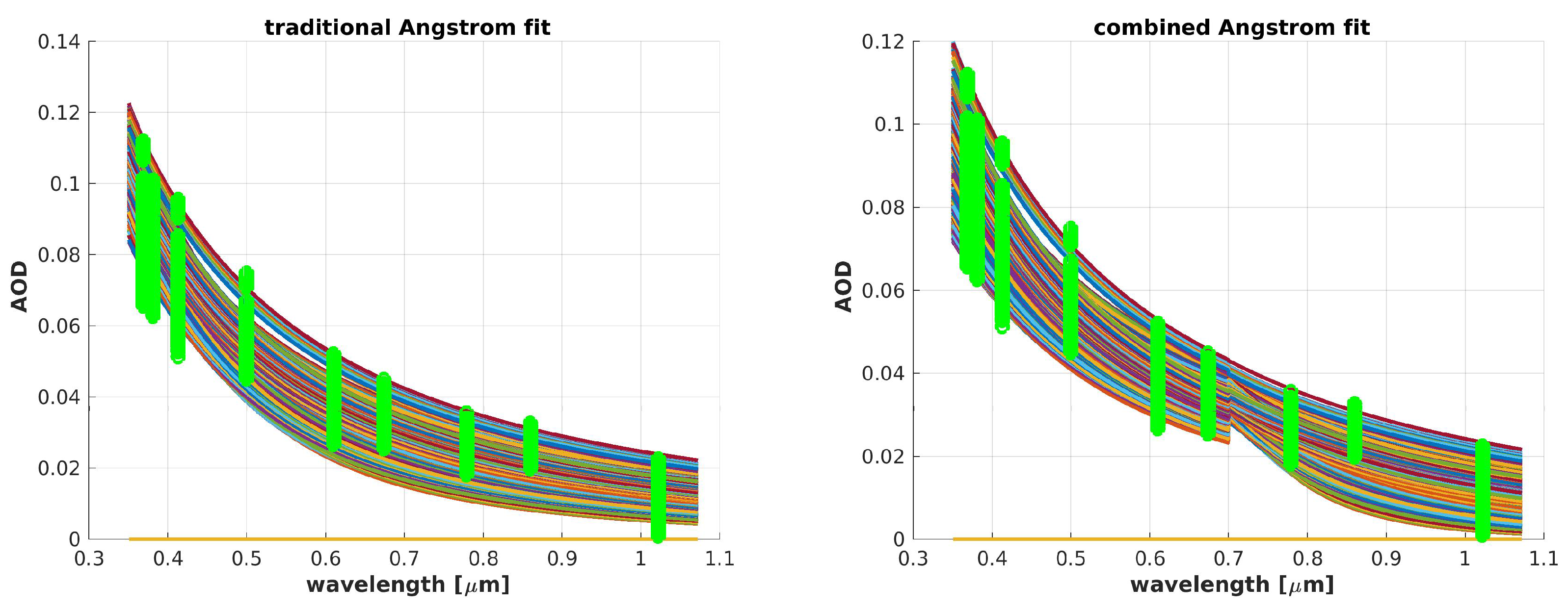
However, the assumption of a power-law for the AOD is clearly only a common approximation. A typical result for Arctic aerosol (green circles) can be as depicted in Figure 1. Equation (1) was used to fit the exponential law (colored lines) to the observation data of the year 2013 (Figure 1, left). It can easily be seen that this approximation under- and over-estimated the measured AOD at some points. To achieve a better result for the same dataset, the wavelength range was divided into two regimes, one for the visible and Ultraviolet (UV) spectrum (<700 nm), the other for the Infrared part (IR) (>700 nm):
Now, two independent Ångström exponents and and both turbidity parameters and were computed, one corresponding tuple for every wavelength regime. This approach closer represents the measurement (see Figure 1, right) as the differences between fitting curves (colored lines) and the measurement data (green circles) were smaller, especially for the ultraviolet and infrared part of the spectrum. In every randomly-selected day, there was a step at nm in the fitting functions of both regimes, and the fitting accuracy was always improved. Therefore, the function of Equation (1) did not give a good approximation of the aerosol properties in the Arctic when applied over a broad spectral region and needed to be improved by a wavelength-dependent Ångström law. Contrary to the data of this work, for other sites with moderate AOD and at least 12 wavelengths, however, it is possible to retrieve significant microphysical properties from the Ångström exponent, as shown e.g., by Cachorro et al. [26].
Already, O’Neill et al. [27] (amongst others) modified the traditional Ångström exponent, via the separation into a fine, f, and a coarse, c, mode to gain additional information about bimodal aerosol size distributions for each wavelength:
where and are the vertically-integrated number density in abundance and , as well as are the extinction cross-sections of the fine and coarse mode. The Ångström exponent is defined as:
with the second derivative:
The total optical curvature parameters , and characterize most of the variability in the AOD spectra according to O’Neill et al. [28]. These parameters are related to the coarse and fine mode components of the measured bimodal aerosol particle size distribution [28]. In O’Neill et al. [29], all three parameters referred to the measured spectrum to the reference values of nm in a second-order polynomial fit of versus to obtain the fitting parameters , , and :
However, a slightly different and easier fitting approach was chosen in this paper. A Taylor expansion of the traditional Ångström exponent of Equation (1) to the first-order correction term leads to the equation:
In the following, is called the modified Ångström exponent, the spectral slope, and F() the total effective Ångström exponent. The physical meaning of this approach is simple: is the classical Ångström exponent in the limit of very short wavelengths (), and gives the wavelength dependence. The turbidity parameter C is treated as a constant. This is in contrast, e.g., to the approach of Shifrin [30]. A wavelength-independent turbidity factor has, however, the advantage that it only depends on the aerosol concentration, not on its microphysical properties. Since 2009, in 254,312 of 255,389 () individual sun photometer measurements, a clearly increased fitting accuracy by the new approach was found. This fitting accuracy is defined by:
where and refer to the measured and fitted AOD value at each of the wavelengths, . The error of the measured AOD () was set to 0.01 for each wavelength, and m are the degrees of freedom.
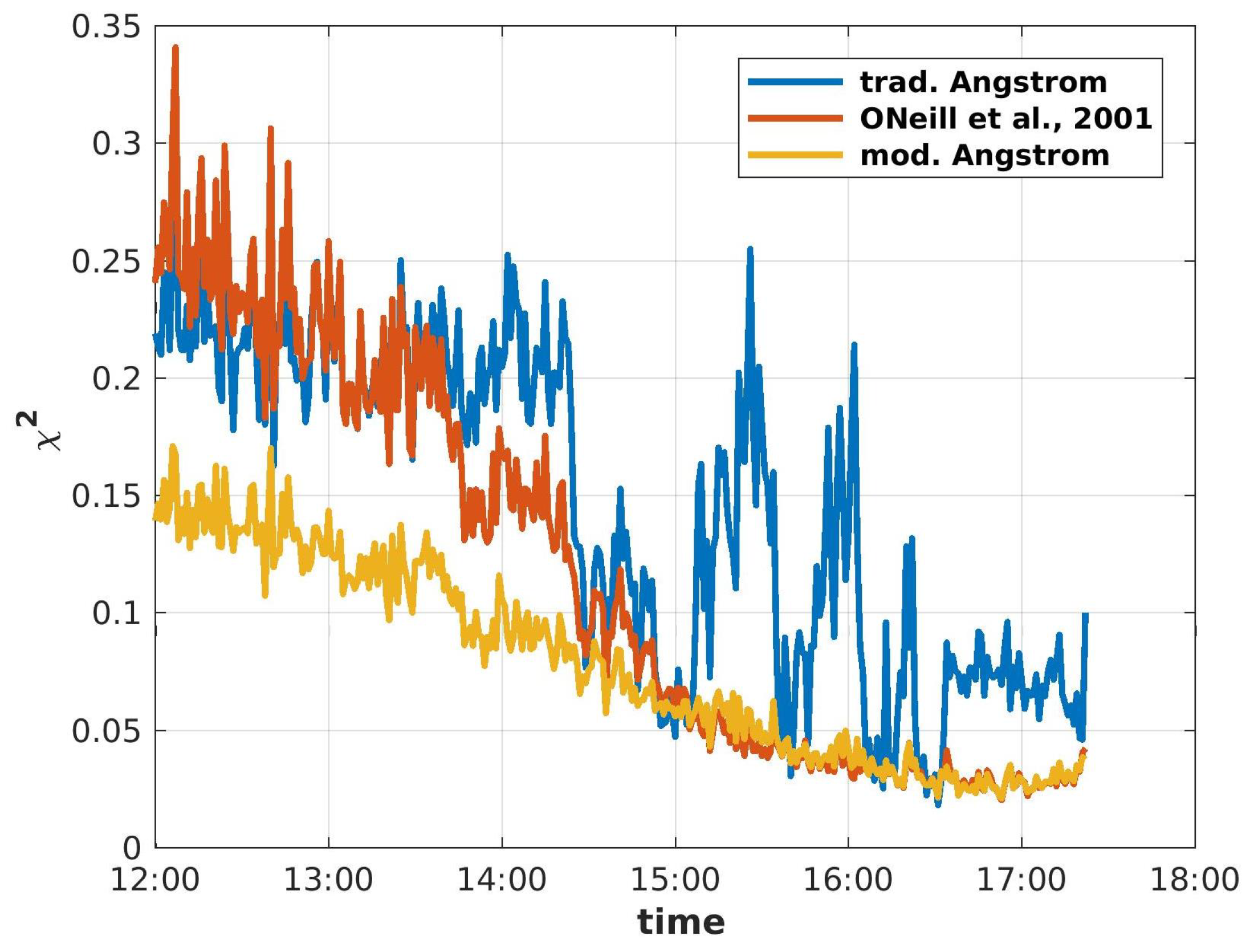
A comparison of the fitting accuracy between the traditional, the modified Ångström law, and the one that was discussed in O’Neill et al. [28] was done for 6 April 2014. The results are presented in Figure 2. A case study including Mie calculus and a comparison with Lidar data for this day is performed afterwards in the Section 3.2.
It can be seen from Figure 2 that for a typical day in spring, both the minute-to-minute fluctuations and the residuals to the observed data were smallest for the modified Ångström approach (yellow) of Equation (5). The fitting accuracy of the traditional Ångström law (Equation (1), red) and the suggestion by O’Neill et al. [27] (Equation (4), blue) were, especially at noon, much poorer than for the approach of Equation (5). The over the afternoon decreasing fitting accuracy, , was a feature of an erroneous Langley calibration [31]. It is worth mentioning that the fitting accuracy of the modified Ångström approach did not change significantly when a thin cloud passed by at 14:30 (see also Section 3.2).
Obviously, the suggested approach with a linear wavelength-dependent Ångström approach fits best for Arctic sun photometer data due to the smallest . For this reason, the so-called “modified Ångström exponent” will be considered most in this paper.
3.1. Mie Calculus
With the Mie program of libRadtran (www.libradtran.org) artificial (ideal) aerosol log-normal distributions were created to get a fully-known aerosol size distribution for the modified Ångström approach. The equation for the log-normal distribution is given in Appendix A. Effective radii between m and m in steps of m were taken, and three different geometrical standard deviations of the distribution widths, , from –1.7 were considered. Refractive indices of and , which are devoted to sulfate-like and strongly-absorbing aerosol-like black carbon, were chosen. The wavelength interval was adjusted to the filters of the sun photometer to [360:1030] nm with a step size of 5 nm. We remark that a similar approach to connect an effective radius of aerosol from photometer data was performed by [32].
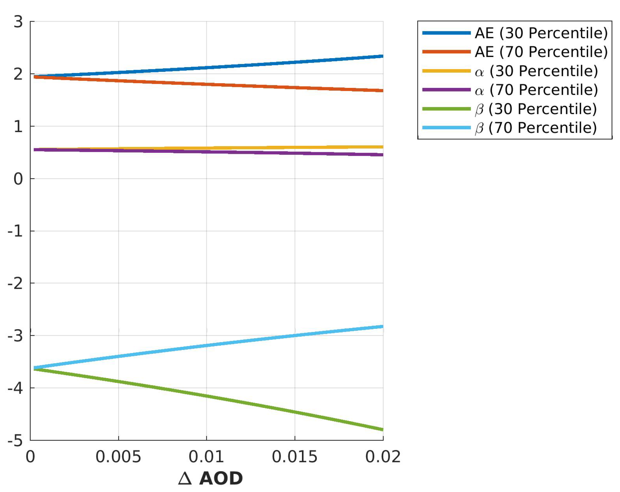
To verify the numerical stability of the modified approach in Equation (5), artificial values of the three parameters C, , and were taken and the resulting AOD calculated. These artificial AOD values were disturbed by 100 different random realizations of noise per noise amplitude AOD. It was checked how an increasing noise level affects the precision by which the crucial parameters and can be retrieved. The result can be seen in Figure 3. Assuming a , which is a typical overall uncertainty for sun photometry (including systematic errors), an error span for the traditional Ångström exponent was found. can be determined better with . The largest uncertainty was stored in with . Later, it will be shown that an error in the AOD of is the maximum to retrieve any information of aerosol microphysical properties from photometer data.
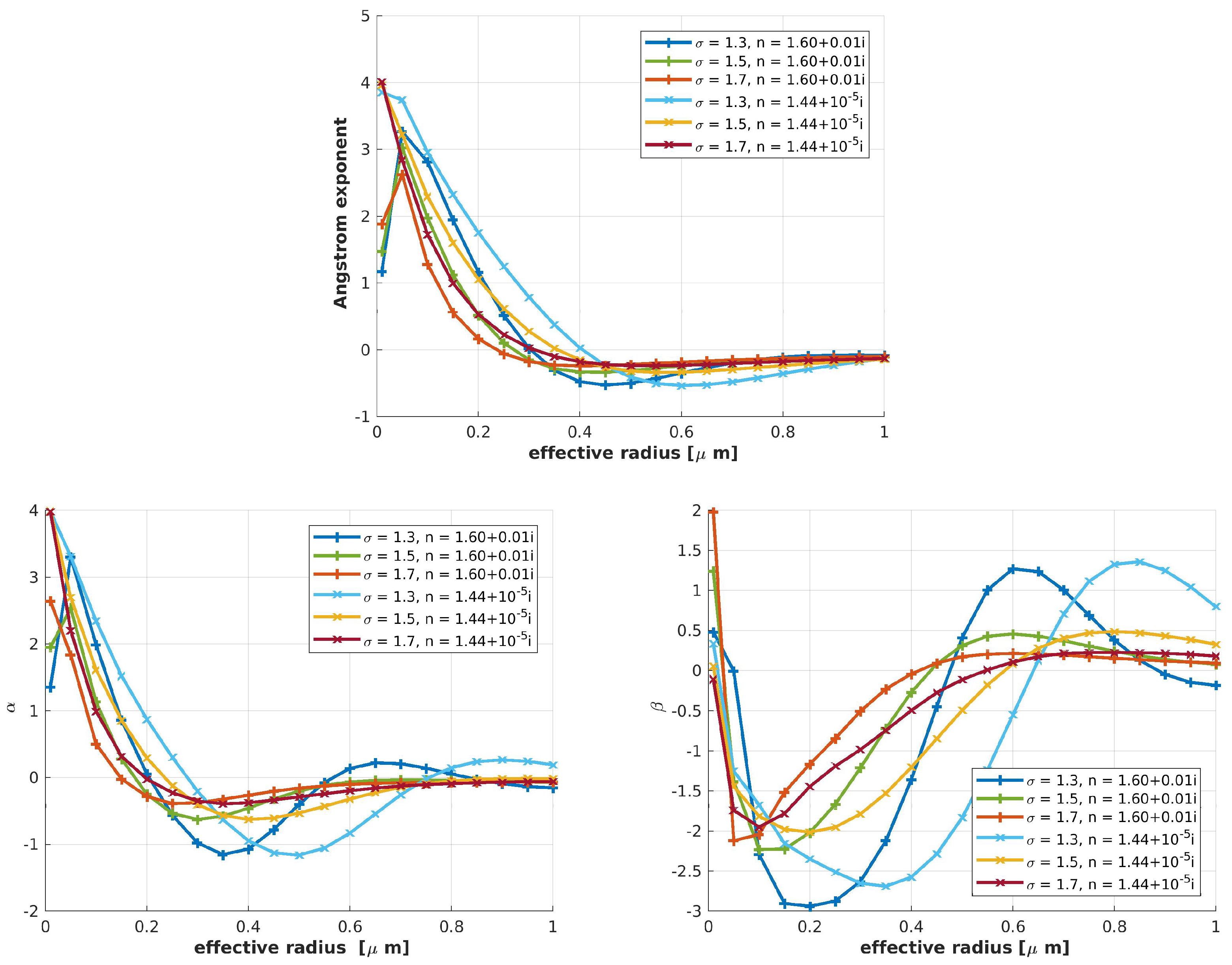
With the above-mentioned parameters and n, the dependency of the Ångström parameters , , and on the effective radius were investigated and are presented in Figure 4. For each value of , , and n, a noise-free AOD was calculated, from which the three Ångström parameters were retrieved.
It can be seen from Figure 4 that already around an effective radius of m, it became difficult to distinguish a given aerosol distribution from the Ångström parameters due to the grey approximation. When the size distribution became wider () or the refractive index was high , the variation of the parameters was less and the grey approximation valid already for smaller effective radii, in agreement with Mie theory, e.g., Hulst [33]. The traditional Ångström exponent did not depend uniquely on the properties of the aerosol distribution. To determine an effective radius of the aerosol distribution using the traditional Ångström law, knowledge of the standard deviation and the refractive index was required. For , even knowledge of and n was not sufficient to determine a unique effective radius from the traditional Ångström exponent (dark blue and green curves in Figure 4).
Contrarily, by the two independent parameters and , some more information can be obtained. The modified Ångström exponent generally behaved similarly to the traditional one. In the Arctic environment, the important size range is m [9]. Only in this radius interval, and monotonically rose for each geometric standard deviation and refractive index. Generally, more narrow aerosol size distributions with low refractive indexes are better suited for the determination of the additionally obtainable information of photometer data, because and changed more strongly over a wider range of effective radii. The spectral slope showed a pronounced variation and even changed its sign, when the effective radius became larger. Typically, two very different effective radii correspond to the one given value of . The independent information of the two parameters, and , can be used to narrow down all possible aerosol size distributions, which were in agreement with the measured Ångström parameters.
A possible solution can only be found if and have the same effective radius within their error margin. Finding only one unique combination of Ångström values additionally gives the standard deviation of the size distribution and the refractive index at the same time. Using other instruments, like in situ instruments or a multiple wavelength Raman Lidar, the refractive index can be determined independently [34,35].
Typical values for the three Ångström parameters for Arctic aerosol are , , and . A possible aerosol size distribution can be identified by using Figure 4. All possible combinations are presented in Table 1, and the most probable results are highlighted in red. A matching of the effective radius can be obtained by comparing the possible solutions for and within their error margin. This example yields either an effective radius m at a standard deviation for or m for and . Even though there were two possibilities using the modified Ångström approach with different refractive indices and the geometric standard deviations, the effective radius of the aerosol can be estimated roughly. On the other hand, there were in total seven possible combinations using the traditional Ångström approach, spanning an interval over more than one order of magnitude for the radius, but only two very similar aerosol distributions using the modified Ångström law.
To conclude, using the traditional Ångström law, one can in general not gain unique information about the distribution or the refractive index. On the other hand, the modified approach provided more information, especially about the effective radius in the size interval between m and m.
3.2. Case Study: Sun Photometer-Lidar
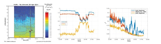
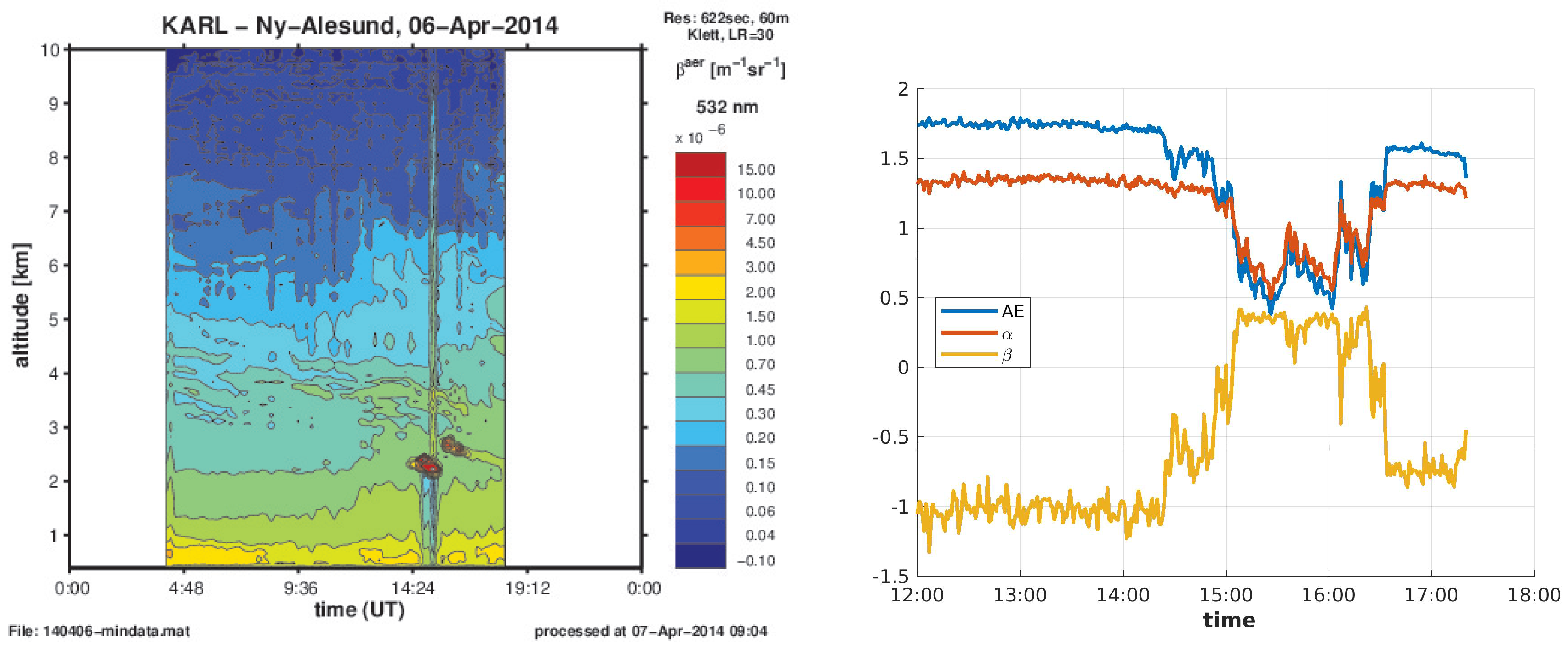
For several days with only briefly appearing clouds, the three parameters , and were compared. In the photometer data (Figure 5, right) on 6 April 2014, the clouds can be recognized easily between 14:30 and 16:30 by the sudden change of all three parameters. With the Koldewey Aerosol Raman Lidar (KARL), located in Ny-Ålesund, as well, aerosol layers and clouds can be recognized by measuring the back-scattered laser beam. KARL was further described in Kulla and Ritter [36].
In the comparison of both instruments, several aspects can be found: Generally, the aerosol in the Arctic is quite small in size, as indicated by the Ångström exponent . This is in agreement with earlier photometer studies [17,20], as well as in situ-measured size distributions by Tunved et al. [9]. A slightly lower modified Ångström exponent , than , was found in photometer data at the same time. The uncertainty of the computation was mostly included in , as can be seen in Figure 3 for noiseless data. Further, the variability of of the photometer measurement was smaller than the variability of the traditional Ångström exponent .
The spectral slope, , was in most of the cases negative for aerosol, which was obviously smaller than m. Therefore, the whole exponent was less negative for the UV and more negative for the IR light compared to the traditional Ångström law. Such behavior is reasonable as the UV light shows the existing particles as larger than the IR light. In clouds, may change its sign. For times with , the wavelength dependency of the modified Ångström exponent became negligible, and hence, .
Note that this day was chosen for the calculation of the deviation between the fitted and observed AOD in Figure 2. During the time when the photometer detected a cloud, the fit of the traditional Ångström exponent was clearly inferior (see the spikes in in Figure 2).
The detection of the cloud in both instruments, Lidar and sun photometer, had a tiny shift in time. First, the photometer detected the change in AOD, then the cloud also passed by the Lidar. This difference can be explained by the different lines of sight. Whereas the Lidar measures in the zenith, the photometer has to follow its light source. In general, the Sun has only a small elevation at this Arctic site, even in summer, and never stands at zenith. This fact makes a comparison between the photometer and Lidar non-trivial. For clouds, the modified and the traditional Ångström exponents nicely followed each other. After the cloud passed by, the traditional Ångström exponent, , and the spectral slope, , changed its intrinsic values slightly, whereas remained constant.
At 13:00, in the photometer profile (Figure 5, left), the values for the three fitting parameters could be read out with and . With the results of the Mie calculus for and of Figure 4, the parameters of the aerosol size distribution were determinable. For this particular case, a standard derivation of , an effective radius m, and a refractive index of were found.
With the Lidar ratio, [37], the aerosol extinction can be calculated from Lidar data, as well. This was used as an indicator of the comparability of both instruments. Using Figure 5, the parameters for cloud thickness m, back-scattering coefficient , and the Lidar ratio sr can be estimated as:
Contrary to the Lidar, the photometer measured . The major difference of both measuring instrument can be caused by the different lines of sight or the spatial distribution and the temporal evolution of the cloud itself.
To conclude, both instruments could be compared if the atmosphere was homogeneous on longer time scales because both instruments always had a different line of sight. However, they could measure different aerosol optical depths due to the temporal and spatial evolution of the cloud or aerosol layer. To get more information out of one instrument, the other can be taken into account.
4. Results
4.1. Trends in the AOD
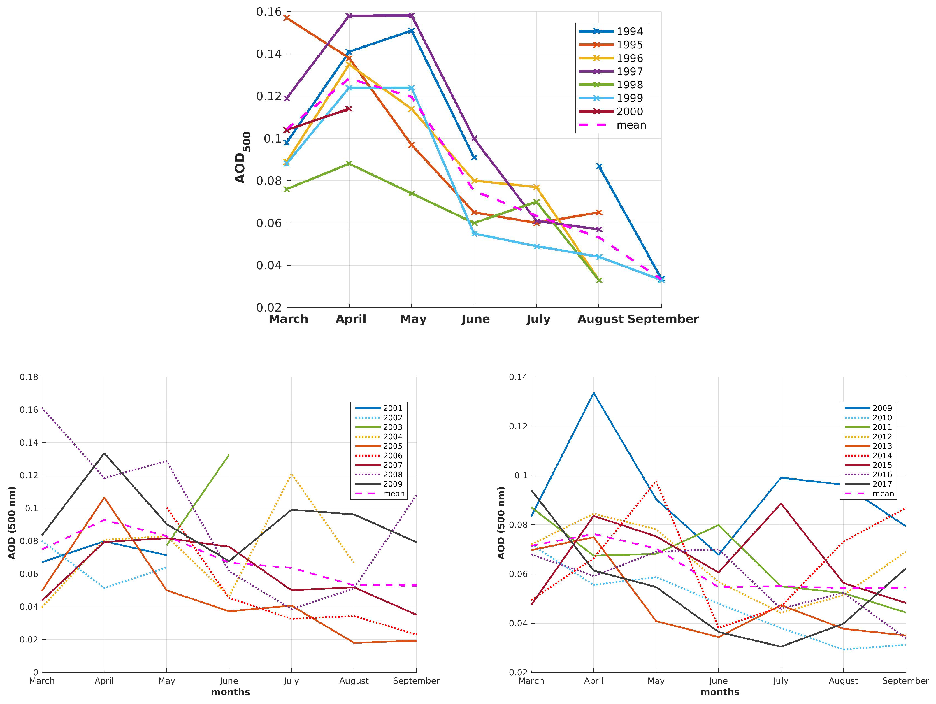
Before showing the multi-annual monthly mean of the of the wavelength nm and its change over time, first, the different annual cycles of the AOD for Ny-Ålesund are presented in Figure 6. A high year-to-year variability was evident. 2009 was the last year with extremely high AOD over the whole year, including the time of the Arctic haze in spring, as well as during the biomass burning season in summer (Figure 6). The high AOD in summer 2009 (June–August) can, however, partially be explained by the eruption of Mt. Sarychev in June 2009. This eruption may have increased the at this site by about 0.05 [38]. The only other volcanic eruption of clear impact on the AOD was Kasatochi in August 2008 [39], which was responsible for the increase of AOD recorded only in autumn 2008. Hence, in spring time, the high AOD of 2009 was purely due to Arctic haze. Comparing both plots in Figure 6, it is evident that the monthly mean AOD decreased over time, as after 2009, no month with was recorded any longer. This was even more remarkable as the data coverage between 2001 and 2004 was poor due to the absence of an automatic tracking system and photometer measurements were more or less only available during campaigns. Hence, monthly means were not available for all months. However, no apparent transition between “polluted earlier years” and “clearer later years” was evident as the inter-annual fluctuations were high. For comparison, the year 2009 was plotted twice. Moreover, in observation data from 1994–2017, it was found that the AOD decreased more strongly in spring and early summer; e.g., in the 1990s, in some years, a high AOD was still found in May. In more recent years, the haze was not only reduced, but also lasted a shorter time during spring. For August and September, the AOD remained almost constant at . This made the annual cycle of the AOD flatter and reduced the importance of the haze season in spring. The trend of both Ångström exponents, and , is plotted in Figure A2 in Appendix C.
With Pearson’s empirical correlation coefficient , it can be shown if two parameters X and Y are statistically correlated:
In the following discussion, the correlation coefficient is applied to the monthly mean AOD trends of the time periods 2001–2009 as X in Equation (7) and for 2009–2017 as Y. An answer, concerning the influence between clear and polluted days on the number of measurement days, can be given with .
For spring (March and April), the correlation was , which indicates a slight anti-correlation. In fact, while the average spring AOD seemed to increase for the earlier period, it had been fluctuating more around a lower value since 2010 (Figure 7). For the other seasons, summer (June–August) and autumn (September), the correlation coefficients were and . Because in both cases, the correlation coefficient , there was no apparent trend for those seasons.
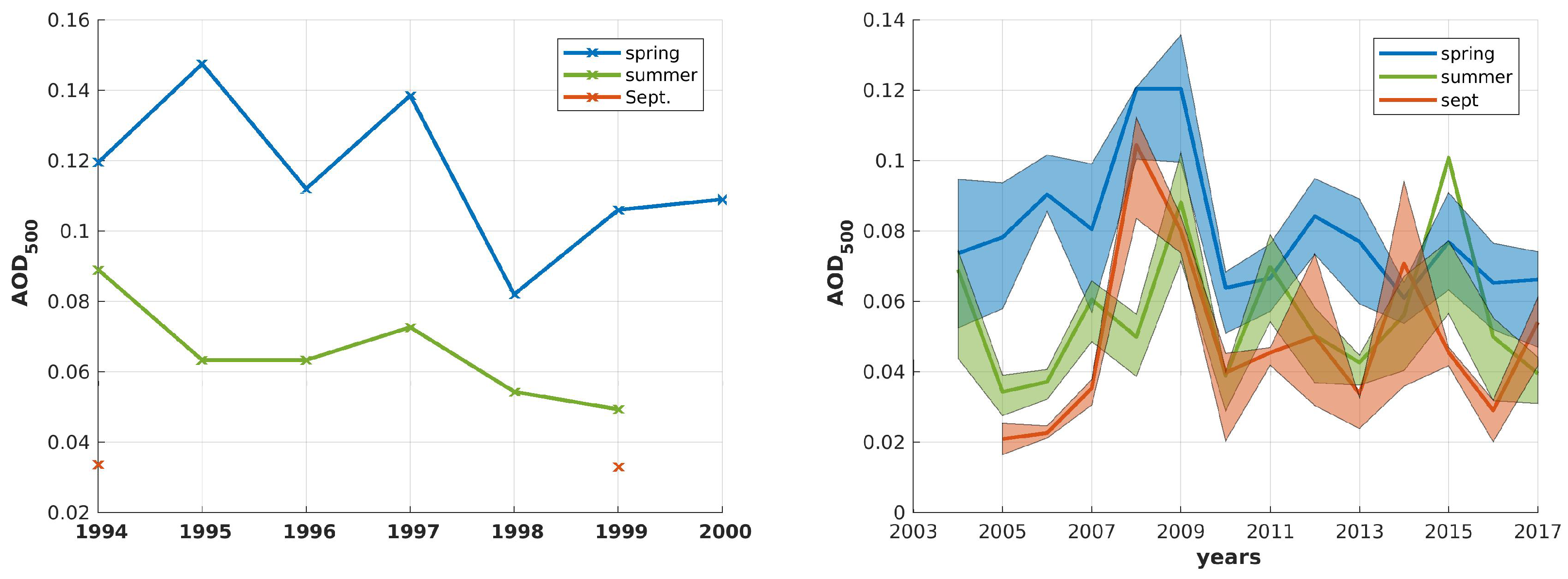
The year-on-year variability of and its variability, expressed by the spread of the 30th and 70th percentile for the different seasons, are shown in Figure 7. Since 1994, the overall decrease of the spring AOD was evident, even if increased during 2004 and 2009. Still, spring is the most polluted season. Furthermore, a quite large spread between the 30th and 70th percentile for the haze season can be seen. This variability means that in each month in spring, both at least one clear, as well as one polluted period were found. Hence, individual haze events lasted less than a month. Hence, in each month in spring, a clear, as well as a polluted period were found. Before 2009, a relative clear monthly average in spring still had a higher AOD than more polluted (70th percentile) averages in summer or autumn, except for only one year of September. The variability in was lower after the haze season in spring. This means that clear or polluted periods seemed to last longer. Finally, it can be seen from Figure 7 that generally, the averaged and the spread were not correlated, although, obviously, a low monthly average also implies a low variability.
With a Nd:YAG laser-based Mie depolarization Lidar system, also located in Ny-Ålesund, a similar pattern of the mean annual cycle of the aerosol load with decreasing importance of the Arctic haze season was recently found [40].
4.2. Histograms of Aerosol Load and Properties
In the previous section, monthly mean values of the were shown in order to present the strong month-to-month variability and the small, but distinct decrease of springtime .
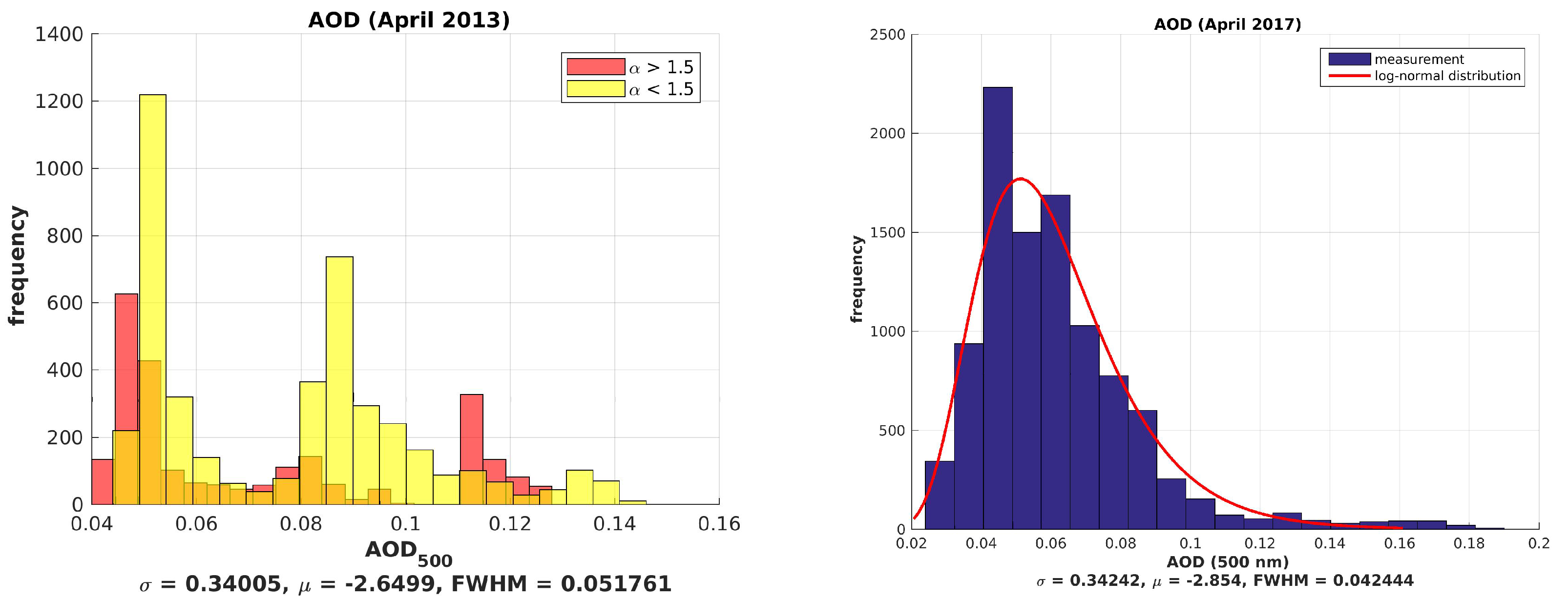
In this section, the minute-by-minute data are analyzed in more detail for some selected periods. Figure 8 shows the histograms of for April 2013 (left) and April 2017 (right). April 2013 was a typical month during the Arctic haze season, as it showed a multi-modal distribution. This means that simple monthly averages, as, e.g., published by Stock et al. [16], are inappropriate. For every month, minute-by-minute data often show a bimodal distribution. This was then used as an indication for large and small aerosol discrimination concerning the modified Ångström exponent in and given in Figure 8. In the segmentation in , the origin of the multi-modal distribution of was obvious as a superposition of small and large aerosol particles having a more or less Ångström exponent. April 2017 is plotted, as well, because it was the only exception with an , as well as a modified Ångström exponent following a mono-modal, log-normal distribution quite well.
Interestingly, the value of the modified Ångström exponent was in general closely related to its spectral slope (Figure 9). The separation of all photometer data into and additionally distinguished between almost negligible () and significant () spectral slope. Due to the definition of the modified Ångström law in Equation (5), the combination of and means that in the UV, a smaller, more negative total effective Ångström exponent was retrieved than for the IR. Similar to the log-normal distributed in April 2017 (Figure 8), the spectral slope, , was distributed following roughly a log-normal distribution (Figure 9), as well.
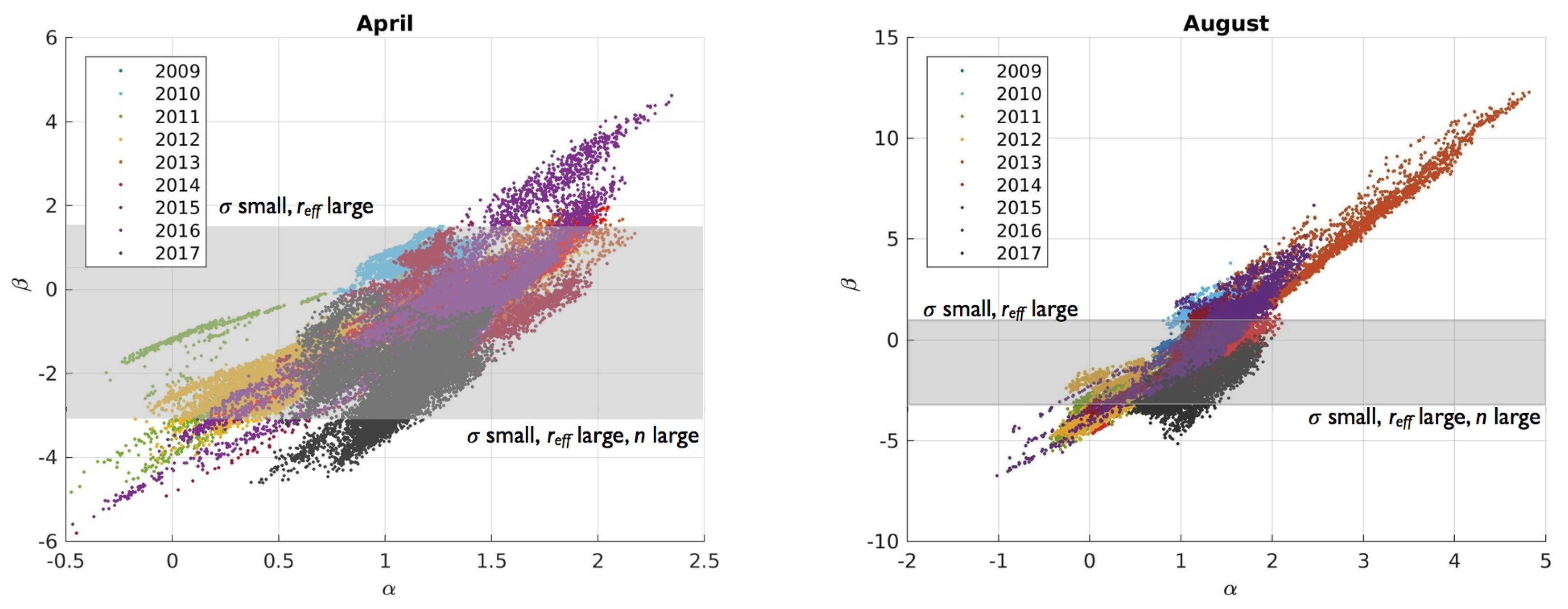
The generally nice correlation between the modified Ångström exponent and its spectral slope is also plotted in Figure 10. The worst correlation between and was found for April 2011 with . The grey shaded area represents the area, where Figure 4 provides results for the assumed choices of the geometric standard deviation of the aerosol size distribution and the refractive index. Beyond this grey area, one cannot get a clear result for the parameters with the one-modal log-normal size distributions and Mie theory mentioned before.
The densest part of Figure 10 (right) remained at the same values for , but slightly shifted to more negative values in in August. While only a smaller range of ( and ) was covered in April, the aerosol became less uniform in summer times ( and ). With this correlation, the effective radius of the underlying aerosol size distributions can be estimated using Figure 4. Preliminary results using the Mie code of libRadtran suggest that large values of may be explained by particles with m. However, a detailed month-by-month analysis of the observed aerosol properties is beyond the scope of this work. As an example, an aerosol size distribution for an refractive index of and a standard deviation of is plotted in Figure A1. The narrower a size distribution gets, the more extreme are the values of . This is a possible explanation for these large values beyond the grey box in Figure 10.
Hence, the aerosol was more heterogeneously distributed in August than in April. On the other hand, the 30th and 70th percentile were quite similar in summer. Therefore, although the measured over the years had about the same absolute value, the composition seemed to be constantly changing from year-to-year during summer and may not be explained by the assumption of spherical particles and a mono-modal log-normal distribution. The aerosol arriving in Svalbard each April was more homogeneous in terms of , , and and may have approximately the same age and similar chemical and physical composition. This is in complete contrast to August, when the aerosol had a lower age, because it was advected more quickly into the Arctic due to a weaker polar vortex, and chemical reactions were still ongoing on the particles. Sources for this kind of aerosol can be biomass burning or marine bionic sulfur emission. In Lidar profiles, such events are shown as individual layers [41]. whereas, the Arctic haze appeared as a constantly higher over the whole part of the lower troposphere [39].
According to Tunved et al. [9], particles are larger within the haze season with typical effective radii of m and smaller particles (m) outside the haze season. If this information is combined with the results of Figure 10 for April and August and the Mie calculations in Figure 4, the size distribution from the ground-based in situ instruments would agree fairly well with the data of this work for April. The range of the modified Ångström exponent, , and its spectral slope, , matched the mono-modal log-normal distributions with particles of effective radius between m. Hence, the ground-based aerosol properties were representative for the whole atmospheric column in spring. However, the wide range of the modified Ångström exponent and its spectral slope in August indicates that during summer, the free troposphere might see a different aerosol load than the surface. Indeed, in the Lidar observations of Shibata et al. [40], an increased backscatter signal was found during summer months up to about an altitude of 5 km.
As in summer, the polar vortex is much weaker than during polar night, much more diverse aerosol can be advected from mid-latitudes into the Arctic. In addition to that, small aerosols produced by plankton and plants are more numerous during polar day. This means that the aerosol is much more diverse in August than in spring, which can be seen in the thresholds between the regimes of high and low AOD (see Table 2) and the larger range in and in Figure 10 with a higher inter-annual variability.
5. Discussion Concerning the Aerosol Origin
5.1. FLEXTRA Five-Day Back-Trajectories
By using five-day FLEXTRA back-trajectories, the origin and the pollution pathway of the aerosol were analyzed to answer the questions about where the aerosol was released into the atmosphere and under which atmospheric conditions the air reached Ny-Ålesund five days later at 500 m, 1000 m, and 1500 m above sea level (asl) at Zeppelin Station. There are some possibilities for how to define trajectory clusters.
First, two different groups were selected depending on the value of the measured . The groups “high AOD” and “low AOD” were defined according to the bimodal distribution of the of the corresponding month. These two groups were each separated afterwards into two additional groups, “dry” and “wet”, depending on whether the relative humidity increased over for at least one time step. Aerosol is highly affected by relative humidity and starts hygroscopically growing after a certain threshold of humidity, which suddenly increases the AOD dramatically. Simultaneously, it is a cloud condensation nucleus and can easily be removed from the atmosphere by precipitation.
Secondly, the ocean, land, and sea ice interact totally differently on aerosols, their origin, and sinks. The influence of the ground conditions was investigated using the fraction of how much time the air stayed over which surface type. Because aerosol is mainly produced on the ground or in the boundary layer, the third way of obtaining information out of the model is by focusing on the time the air resided in the boundary layer.
5.1.1. Aerosol Origin Due to Arriving Air Pollution
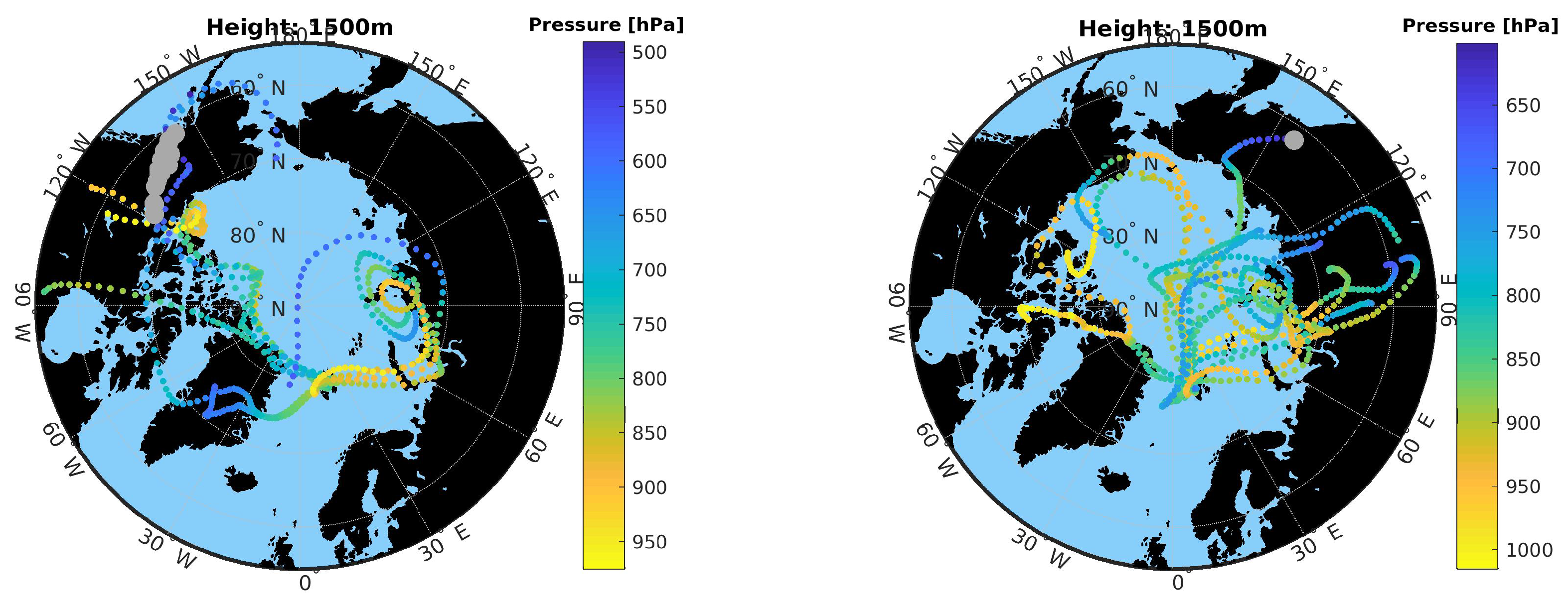
In Figure 11, all 14 trajectories are shown for April 2013, which end at a 1500 m altitude above Zeppelin Station. The multi-modal AOD distributions were considered only showing back-trajectories with low or high AOD. The threshold was determined by the sun photometer, and it was set for each month individually (see Table 2).
For both groups, “high AOD” and “low AOD”, the air may come either from the North American or Russian Arctic. Overall, the trajectory groups looked quite similar. Both groups contained air masses being advected at low altitudes over the American or Eurasian continent. Moreover, precipitation (thick grey dots in Figure 11) did not occur frequently in the trajectory dataset. Hence, one cannot simply assess one single pollution transport or favor one special source region, from which the Arctic haze originated. Note that in this sample, there was no direct transport from Europe. In general, the photometer can only measure during clear-sky conditions, and even thin clouds disturb the measurement significantly. Due to the prevalent west-wind drift, much moist air is transported from the Atlantic to Svalbard, shielding Europe. Therefore, in the photometer data, there was always a bias in the data with an under-representation of Northern Europe, as well as the Atlantic being the pathway of precipitation-bringing areas. Hence, aerosol from Europe may enter the Arctic mainly in interstitial form. Although the European origin of inert trace gases arriving in Ny-Ålesund has already been proven [42], this is not possible for aerosols yet. When they enter clouds, aerosols change their physical and chemical properties. Because they act as cloud condensation nuclei, they form droplets and are washed out by precipitation. For this reason, they do not have exactly the same pollution pathways into the Arctic as trace gases, and determining their origin with models becomes much more difficult. Especially in the Arctic, the interaction between clouds and aerosol, as well as their lifetime in the atmosphere are only poorly understood.
The plotted trajectories in Figure 11 show only one example of high and low AOD for a typical month and year. In April 2013, the air came from Siberia, as well as from North America and Greenland, being dry, as well as wet and reaching heights of up to 500 hPa. Because no bi-modal distribution in was found in April 2017, no distinction in high and low AOD can be made. This year was omitted for trajectory analysis. Similar to Figure 11, trajectories for many more months inside and outside the Arctic haze season have been calculated.
One can say that the origin of air with low AOD comes slightly more frequently from North America, whereas air with high AOD has a higher probability to originate from Siberia. However, in both cases, there are also many trajectories coming from the other continents before reaching Svalbard. Hence, any clear source region of the aerosol was not found. Furthermore, the pattern of each chosen height looked similar. Hence, the dependency of the chosen height was not the most important point of the interpretation of back-trajectories. Maybe the biggest problem is the reliability of the wind fields, especially at high latitudes.
Contrary to this approach and dataset, Christensen et al. [43] and Udisti et al. [5] employed a chemical analysis of aerosol in situ measurements from Ny-Ålesund to perform a source apportionment for the important sulfate component of the Arctic haze. They found a clear anthropogenic origin for data from April and more marine aerosol during summer. Clearly, looking for markers in in situ samples is one way to prove the origin of Arctic aerosol. However, its pollution pathway and lifetime in the atmosphere remain open questions.
5.1.2. Aerosol Sources and Sinks
As the five-day back-trajectory analysis did not show any convincing source region of Arctic haze, the following hypothesis was tested: Does the time the air parcel spends over sea ice, free ocean, or land have an impact on low and accordingly high AOD in Ny-Ålesund? Does the measured AOD depend more on the effective sinks instead of sources?
The albedo of sea ice and snow covered land is very high, and heating of the ground by the Sun is very inefficient. Hence, the atmosphere is thermodynamically stably stratified, and the boundary layer is thin. Therefore, it is expected to have less vertical mixing, a dry boundary layer and, therefore, a longer aerosol lifetime compared to air masses being advected over the free ocean. Due to this initial condition, aerosol sinks are turned off over ice, and the aerosol can mainly be transported, not removed.
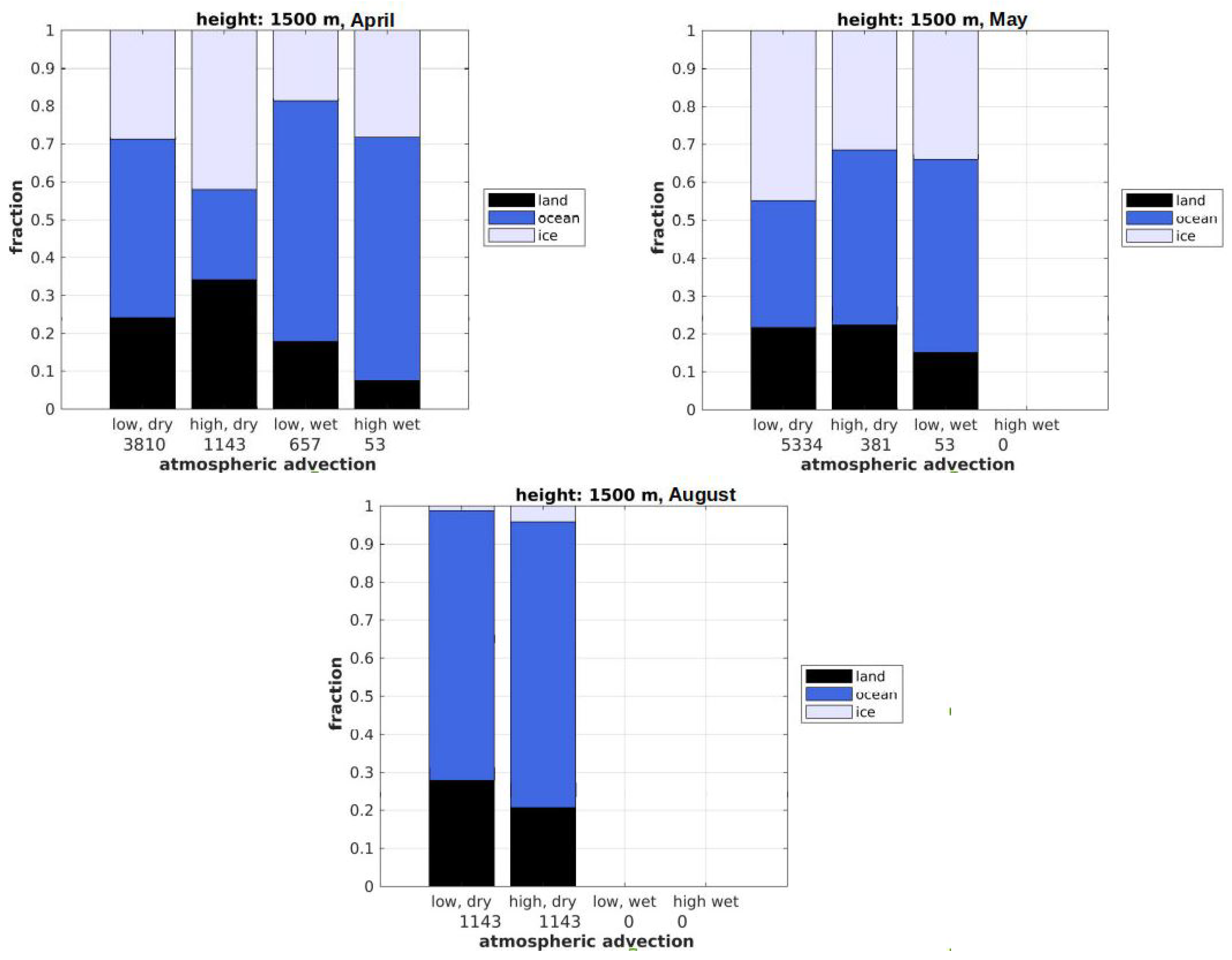
This idea was checked by the fraction of time the air parcel stayed over land, sea ice, or open ocean, and it was plotted for the month of April 2013 to exemplify it (see Figure 12). Furthermore, the cases “dry” and “wet” air were distinguished using relative humidity > for at least 6 h as a limit and divided between arrival altitudes at 500 m, 1000 m, and 1500 m over Zeppelin Station, Ny-Ålesund. As is known from Lidar observations, the Arctic haze phenomenon usually occurs in the lower troposphere [17,37]. The number of measurements for the so-called “wet” case was much less than for “dry” ones either because the aerosol advection intrinsically occurs in dry air or due to the clear sky bias in the instrument. Cases of wet air below 1000 m altitude drastically reduced the number of available photometer measurements. This is in agreement with Maturilli and Ebell [1], who derived from ceilometer observations that the cloud bottom at Ny-Ålesund was generally below a 1000 m altitude. From this follows that aerosol above a 1000 m altitude may survive cloud formation and is not being washed out. Therefore, it can be measured with photometers in their intrinsic appearance. Due to the annual changes of sea ice extent, the fraction of sea ice in August is always smaller than in April and May, and vice versa for the fraction of the ocean (Figure 12).
The fraction of sea ice was much higher (up to in April) for the “high, dry” case. On the other hand, the category “ocean” had only a fraction of for the case “high, dry”, which was the smallest of all categories (Figure 12). This indicates that the sinks are important. Over sea ice, the boundary layer is stably stratified, and no convection takes place due to the high surface albedo. Additionally, the probability of cloud formation is reduced because convection and moist air are needed. The often occurrence of sea ice acting as a cover of sinks prevents a deposition of the aerosol, and the polluted air is advected by long-range transport. In agreement with Christensen et al. [43] and Tunved et al. [9], aerosol of marine origin can be neglected for optical measurements in the haze season. Furthermore, the explicit consideration of aerosol sinks might be very important to understand the advection into the Arctic. Whereas, the boundary layer is stably stratified over the sea ice and the efficiency of sinks is reduced, the probability of cloud formation is much more likely over a convective boundary layer over the ocean with moist conditions.
Due to a higher probability of wet deposition in summer than in winter, the mean lifetime of aerosol is much shorter. Therefore, the results of the trajectory model should be more reliable in summer than in winter times. A tendency of the surface fraction can be seen: the longer the air was over sea ice, the higher was the AOD, e.g., in April, the ice fraction for the case “low, dry” was , whereas it was for the case “high, dry”. The sea ice reduced the efficiency of sinks. For April and May, it seemed that the high AOD was additionally caused by a high fraction of land, because most of the aerosol was released there in the presence of plants, humans, and soil.
5.1.3. Remarks on the Advection Altitude
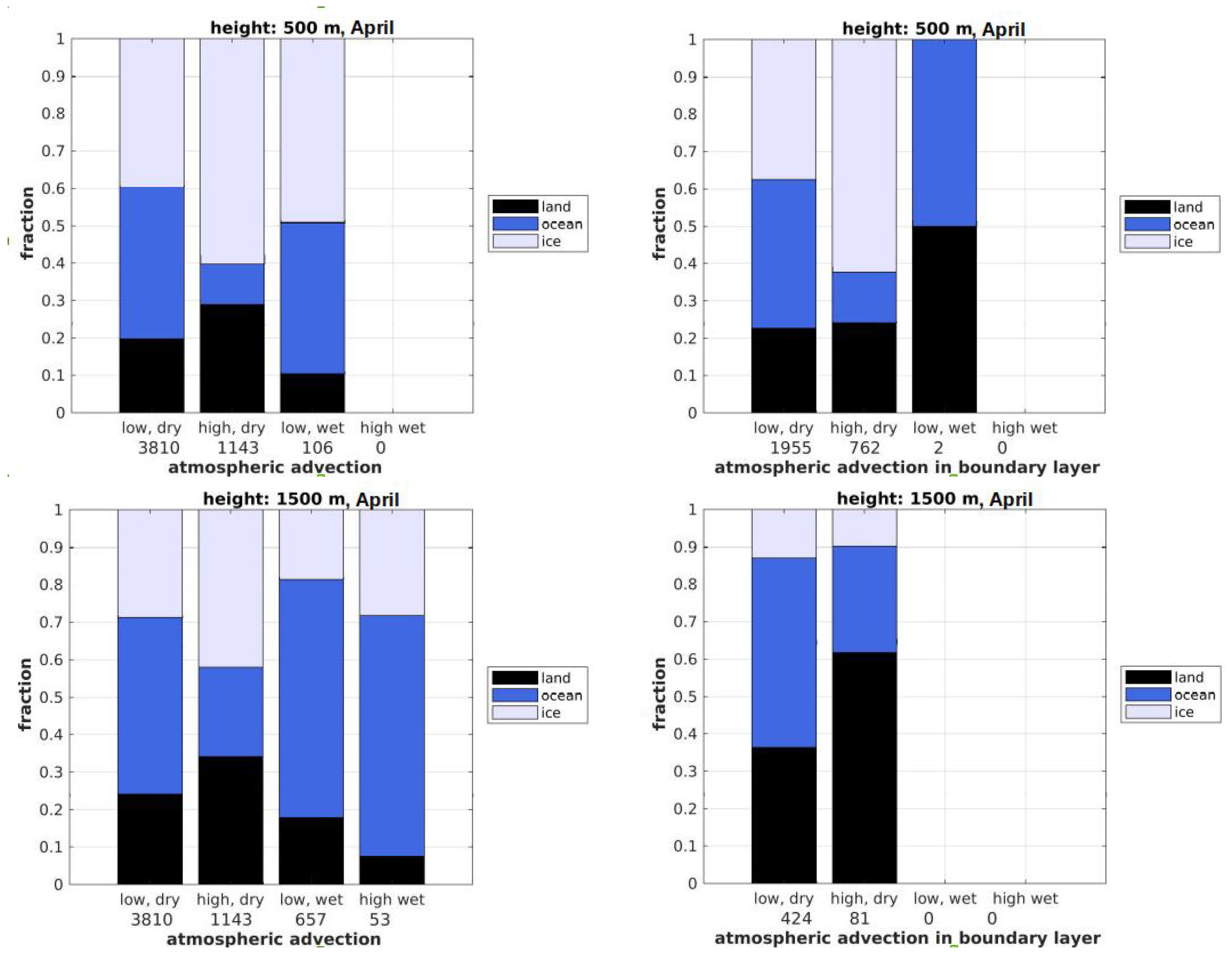
A clear difference can be seen in Figure 13 for each height and type of ground (land, free ocean, or sea ice). The left plots of Figure 13 and Figure 14 represent all data independent of the height the air was on the way to Zeppelin Station, whereas the plot on the right only shows trajectories, for which the air was in contact with the ground (minimum 2 h) at the lowermost 100 hPa pressure level, which is called the “boundary layer” in the following discussion.
Air parcels arriving at 500 m above the station are easily influenced by the local boundary layer, or even are still part of it. Whereas the sea ice content of the Arctic is close to its maximum in April, the air likely flows near the ground. Due to friction, the wind speed in the boundary layer is smaller than in the free troposphere above, which means the air cannot flow such long distances within the five days of the calculated back-trajectories. Therefore, the differences between low and high AOD for the boundary layer were due to the reduced sinks over ice. Contrarily, in the case of all trajectories and a 500 m arrival height, the difference between “high” and “low” AOD is both due to more aerosol uptake over land (sources) and reduced sinks over ice. Air parcels being close to the ground and over continents have to travel a long distance in only five days to reach Spitsbergen. Therefore, the air has to ascend and reach the free troposphere with higher wind speeds. This air mainly remains at a higher altitude and arrives over Zeppelin Station more often at 1500 m. With the influence of the orography of the surrounding continents, the air reaches the needed height. However, these possibilities are not available over sea ice, which why this fraction is the smallest (Figure 13, bottom right). Because, typically, clouds lie below the arriving height of the back-trajectories at 1500 m [1], the aerosol is not washed out after it arrives in the free troposphere.
In the “wet” cases, the high relative humidity changed the aerosols and their optical properties. Therefore, the sources lost their importance in the contribution of high or low AOD measured at Ny-Ålesund. For these trajectories, the presence of sinks is more important.
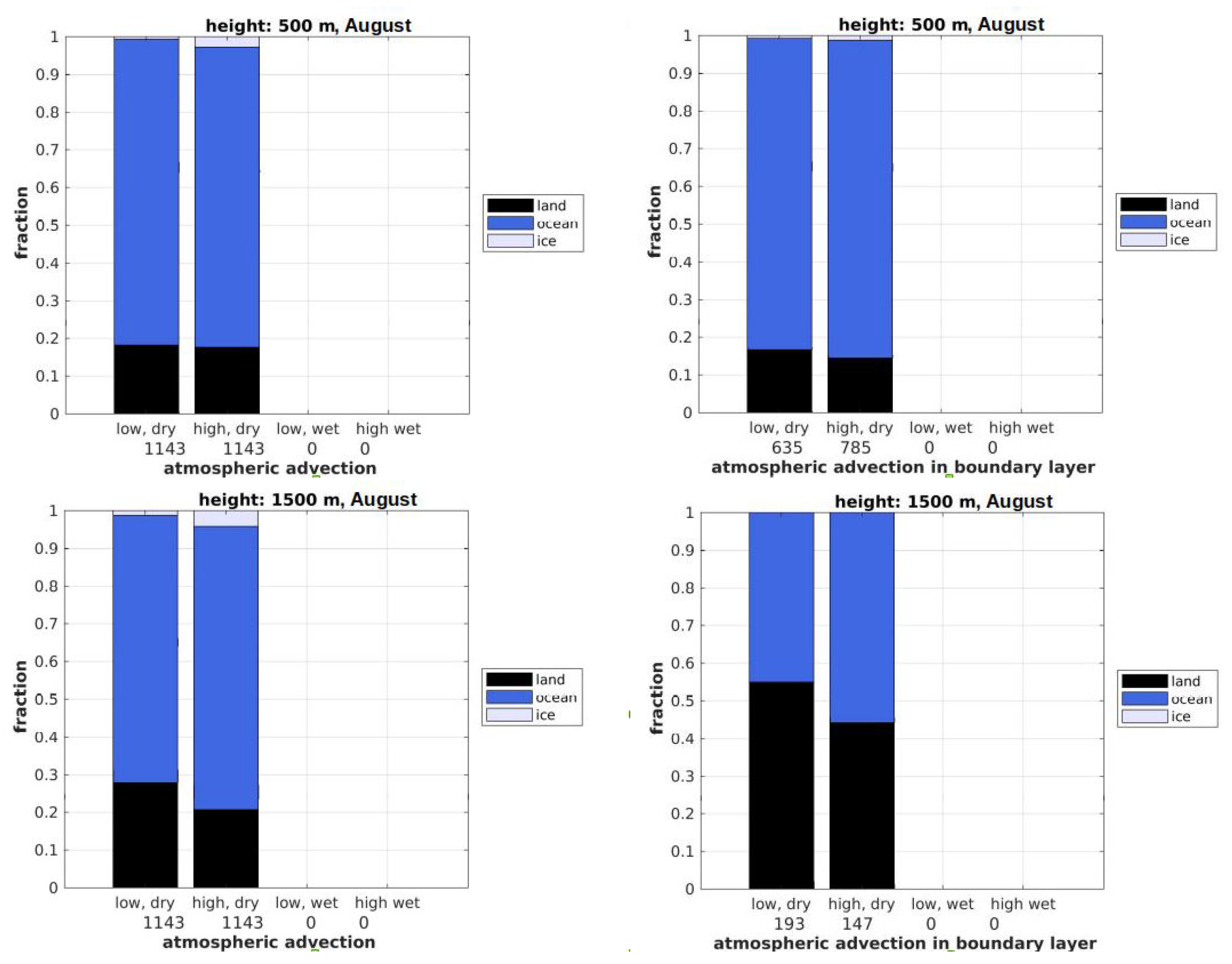
For August (Figure 14), the situation looked different than for April. Due to the annual minimum, the sea ice concentration was very low, and a concentration of of sea ice in one grid cell of the ERA-Interim re-analysis model was reached for only a few cases. As for the cases in April, the fraction of land rose with the arriving altitude of the air parcel, while the fraction of the ocean was decreasing at the same time. Compared to April, the situation looked completely different, because there was no deviation between the fractions for the whole atmosphere and the boundary layer. Moreover, for August, the difference between advection over the ocean and the continent decreased. This can be explained in two ways: First, contrary to spring time, the Arctic Ocean can be a source of aerosol in summer due to DMS production (Dimethylsulfide) Udisti et al. [5]. Hence, the role as the ocean being only a sink for aerosol might not be so clear during summer. Second, due to the results of the previous section, the aerosol might be more diverse and arrive at higher altitudes during summer [40].
To get a better estimation of the error, back- and forward-trajectories have to be considered. Whereas back-trajectories have one exact starting point, forward-trajectories should be set into a grid around the position where the back-trajectories ended. In case the model has a sufficient resolution, the forward-trajectories will end at approximately the same area as the ones that were back-computed.
However, another reason for the insufficient result of the model can be the aerosol lifetime. During winter times, most of the ground at high latitudes is covered by snow and ice. The snow prevents dry deposition, and the aerosols can remain on average about 15 days in the atmosphere before they are sedimented [44]. However, for this long time, the uncertainties of the model are way too large to gain information from this approach.
6. Conclusions
In this paper, an improvement of the fitting approach for photometer data was presented taking into account the first-order term of the Taylor extension of the Ångström exponent. Hence, this new approach was wavelength dependent. It was found that the modified and slope were correlated, which means larger particles had a smaller spectral slope .
Additionally, the information content behind photometer data using the modified approach with and has been assessed using the Mie program of libRadtran. Whereas the traditional Ångström exponent hardly allows any information on the particle size, via the new approach, a typical effective radius for spring time may be in the order of m, whereas in summer, the aerosol properties are more diverse and sometimes cannot be explained by Mie theory and a one-modal log-normal distribution.
Within the measurement data starting from 1994–2017, a declining trend in AOD of the Arctic haze during the spring months (March and April) was found with a simultaneously strong year-on-year variability. For every month, the minute-by-minute data normally showed a bi- or even multi-modal distribution of the AOD. The was slightly declining in spring months; on the other hand, it increased in autumn at the same time, which makes the annual cycle of AOD flatter. The spread between the 70th and 30th percentile of AOD was generally large during the Arctic haze season, which means that in spring, typically both clear and polluted days occurred each month. Apparently, mainly the aerosol load changed, not the aerosol properties, which may agree with the measurements on the ground in the atmospheric column.
No evident origin was found for high or low polluted air arriving at Ny-Ålesund using FLEXTRA five-day back-trajectories. Because of the clear sky bias, most of the precipitating advecting air masses had not been recorded by the sun photometer. The aerosol pathway through the atmosphere is an open question, but needs to be solved by more reliable reanalysis datasets.
An indication was found that sea ice acting as the reduction of aerosol sinks controls the AOD in the European Arctic during spring. The decline of Arctic haze can probably be related to more efficient aerosol sinks, for example caused by the shrinking ice cover. When using back-trajectories, sinks and sources are equally important to consider. Therefore, in case the arriving air carries a high amount of pollution and is not being washed out by precipitation, the air can be either advected over sea ice or arrive at an altitude above 1000 m, which is over the average height of polar clouds.
Author Contributions
This work was basically performed by S.G. C.R., as PI of the instruments, acted as the supervisor.
Funding
The authors did not receive any external funding.
Acknowledgments
The photometer was serviced at Ny-Ålesund by Jürgen Graeser and calibrated (Tenerife), as well as its data checked (Potsdam) by Siegrid Debatin. Two anonymous reviewers improved the quality of this work by constructive remarks.
Conflicts of Interest
The authors declare no conflict of interest.
Appendix A. Definition of the Aerosol Distribution
To generate an aerosol size distribution for the Mie calculus, the following log-normal distribution was chosen:
where N is the number of particles or size r, is the mean radius, and the geometrical standard deviation. libRadtran considers one particle per cm as the default. The effective radius can then be obtained from the aerosol distribution by:
Appendix B. Additional Mie Calculus
Figure A1 shows the three parameters of the traditional and modified Ångström laws, , , and , for a very narrow aerosol size distribution and a refractive index of . One can easily see that the narrower a distribution gets, the larger the difference of to gets.
Figure A1.
Mie calculus for a homogeneous aerosol layer with a refractive index on and a standard deviation of .
Figure A1.
Mie calculus for a homogeneous aerosol layer with a refractive index on and a standard deviation of .

Appendix C. Trend of Both Modified Ångström Exponents
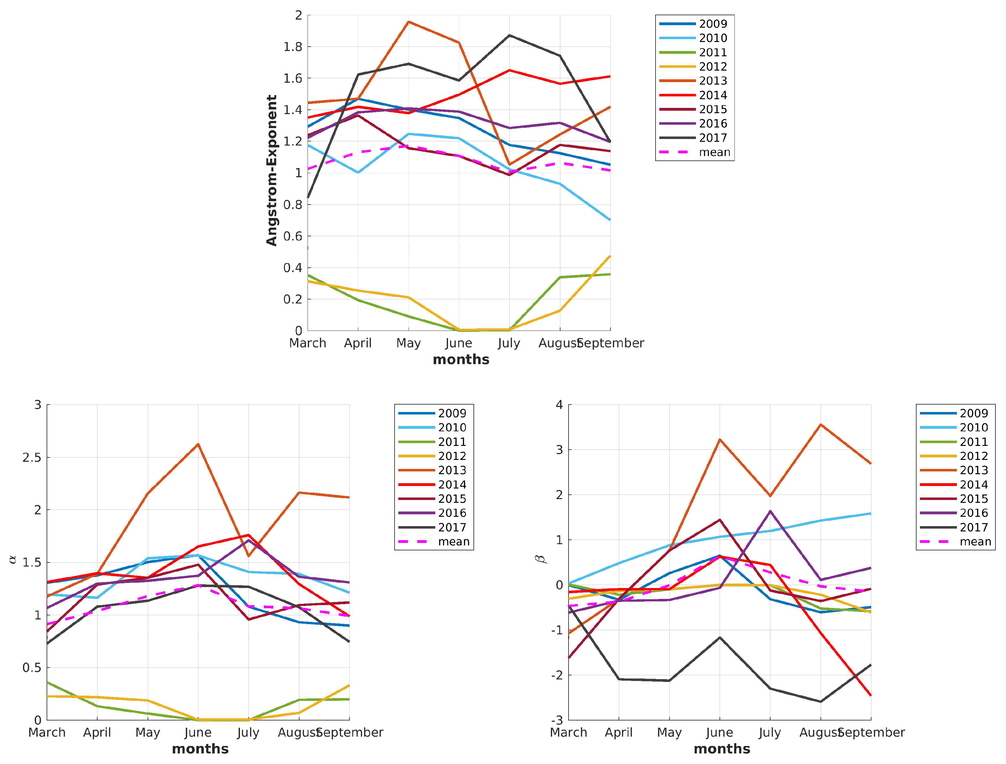
In Figure A2, the long-term series of the traditional and modified Ångström exponents, , , and , is plotted for the years 2009–2017. No reason was found why the mean values for and had opposite signs in the years 2011 and 2012. As the AOD for those years seemed to be normal, no hints for calibration or pointing issues were found. It is remarkable that the mean annual cycle of (pink, dashed) matched the in situ observation at the site.
Figure A2.
Trend of the traditional and modified Ångström exponents (upper row), , and (lower row) for the years 2009–2017.
Figure A2.
Trend of the traditional and modified Ångström exponents (upper row), , and (lower row) for the years 2009–2017.

References
- Maturilli, M.; Ebell, K. Twenty-five years of cloud base height measurements by ceilometer in Ny-Ålesund, Svalbard. Earth Syst. Sci. Data 2018, 10, 1451–1456. [Google Scholar] [CrossRef]
- Shaw, G.E. The Arctic haze phenomenon. Bull. Am. Meteorol. Soc. 1995, 76, 2403–2414. [Google Scholar] [CrossRef]
- Quinn, P.; Shaw, G.; Andrews, E.; Dutton, E.; Ruoho-Airola, T.; Gong, S. Arctic haze: current trends and knowledge gaps. Tellus B Chem. Phys. Meteorol. 2007, 59, 99–114. [Google Scholar] [CrossRef] [Green Version]
- Hara, K.; Yamagata, S.; Yamanouchi, T.; Sato, K.; Herber, A.; Iwasaka, Y.; Nagatani, M.; Nakata, H. Mixing states of individual aerosol particles in spring Arctic troposphere during ASTAR 2000 campaign. J. Geophys. Res. Atmos. 2003, 108, 4209. [Google Scholar] [CrossRef]
- Udisti, R.; Bazzano, A.; Becagli, S.; Bolzacchini, E.; Caiazzo, L.; Cappelletti, D.; Ferrero, L.; Frosini, D.; Giardi, F.; Grotti, M.; et al. Sulfate source apportionment in the Ny-Ålesund (Svalbard Islands) Arctic aerosol. Rend. Lincei 2016, 27, 85–94. [Google Scholar] [CrossRef]
- Warneke, C.; Bahreini, R.; Brioude, J.; Brock, C.; De Gouw, J.; Fahey, D.; Froyd, K.; Holloway, J.; Middlebrook, A.; Miller, L.; et al. Biomass burning in Siberia and Kazakhstan as an important source for haze over the Alaskan Arctic in April 2008. Geophys. Res. Lett. 2009, 36, L02813. [Google Scholar] [CrossRef]
- Markowicz, K.M.; Pakszys, P.; Ritter, C.; Zielinski, T.; Udisti, R.; Cappelletti, D.; Mazzola, M.; Shiobara, M.; Xian, P.; Zawadzka, O.; et al. Impact of North American intense fires on aerosol optical properties measured over the European Arctic in July 2015. J. Geophys. Res. Atmos. 2016, 121, 14,487–14,512. [Google Scholar] [CrossRef] [Green Version]
- Park, K.T.; Jang, S.; Lee, K.; Yoon, Y.J.; Kim, M.S.; Park, K.; Cho, H.J.; Kang, J.H.; Udisti, R.; Lee, B.Y.; et al. Observational evidence for the formation of DMS-derived aerosols during Arctic phytoplankton blooms. Atmos. Chem. Phys. 2017, 17, 9665–9675. [Google Scholar] [CrossRef] [Green Version]
- Tunved, P.; Ström, J.; Krejci, R. Arctic aerosol life cycle: Linking aerosol size distributions observed between 2000 and 2010 with air mass transport and precipitation at Zeppelin station, Ny-Ålesund, Svalbard. Atmos. Chem. Phys. 2013, 13, 3643–3660. [Google Scholar] [CrossRef]
- Dubovik, O.; Holben, B.; Eck, T.F.; Smirnov, A.; Kaufman, Y.J.; King, M.D.; Tanré, D.; Slutsker, I. Variability of absorption and optical properties of key aerosol types observed in worldwide locations. J. Atmos. Sci. 2002, 59, 590–608. [Google Scholar] [CrossRef]
- Li, S.; Kahn, R.; Chin, M.; Garay, M.; Liu, Y. Improving satellite-retrieved aerosol microphysical properties using GOCART data. Atmos. Meas. Tech. 2015, 8, 1157–1171. [Google Scholar] [CrossRef] [Green Version]
- Mei, L.; Xue, Y.; de Leeuw, G.; von Hoyningen-Huene, W.; Kokhanovsky, A.A.; Istomina, L.; Guang, J.; Burrows, J.P. Aerosol optical depth retrieval in the Arctic region using MODIS data over snow. Remote Sens. Environ. 2013, 128, 234–245. [Google Scholar] [CrossRef]
- Herber, A.; Thomason, L.W.; Gernandt, H.; Leiterer, U.; Nagel, D.; Schulz, K.H.; Kaptur, J.; Albrecht, T.; Notholt, J. Continuous day and night aerosol optical depth observations in the Arctic between 1991 and 1999. J. Geophys. Res. Atmos. 2002, 107, AAC 6-1–AAC 6-13. [Google Scholar] [CrossRef]
- Rozwadowska, A.; Zieliński, T.; Petelski, T.; Sobolewski, P. Cluster analysis of the impact of air back-trajectories on aerosol optical properties at Hornsund, Spitsbergen. Atmos. Chem. Phys. 2010, 10, 877–893. [Google Scholar] [CrossRef] [Green Version]
- Toledano, C.; Cachorro, V.; Gausa, M.; Stebel, K.; Aaltonen, V.; Berjón, A.; de Galisteo, J.O.; De Frutos, A.; Bennouna, Y.; Blindheim, S.; et al. Overview of sun photometer measurements of aerosol properties in Scandinavia and Svalbard. Atmos. Environ. 2012, 52, 18–28. [Google Scholar] [CrossRef]
- Stock, M.; Ritter, C.; Aaltonen, V.; Aas, W.; Handorf, D.; Herber, A.; Treffeisen, R.; Dethloff, K. Where does the optically detectable aerosol in the European Arctic come from? Tellus B Chem. Phys. Meteorol. 2014, 66, 21450. [Google Scholar] [CrossRef]
- Tomasi, C.; Kokhanovsky, A.A.; Lupi, A.; Ritter, C.; Smirnov, A.; O’Neill, N.T.; Stone, R.S.; Holben, B.N.; Nyeki, S.; Wehrli, C.; et al. Aerosol remote sensing in polar regions. Earth-Sci. Rev. 2015, 140, 108–157. [Google Scholar] [CrossRef] [Green Version]
- Maturilli, M.; Herber, A.; König-Langlo, G. Surface radiation climatology for Ny-Ålesund, Svalbard (78.9 N), basic observations for trend detection. Theor. Appl. Climatol. 2015, 120, 331–339. [Google Scholar] [CrossRef]
- Pakszys, P.; Zielinski, T.; Markowicz, K.; Petelski, T.; Makuch, P.; Lisok, J.; Chilinski, M.; Rozwadowska, A.; Ritter, C.; Neuber, R.; et al. Annual changes of aerosol optical depth and Ångström exponent over Spitsbergen. In Impact of Climate Changes on Marine Environments; Springer: Berlin, Germany, 2015; pp. 23–36. [Google Scholar]
- Stock, M. Charakterisierung der troposphärischen Aerosolvariabilität in der europäischen Arktis [Characterization of Tropospheric Aerosol Variability in the European Arctic]. Ph.D. Thesis, University of Potsdam and Alfred Wegener Institute, Helmholtz Centre for Polar and Marine Research, Potsdam, Germany, 2010. [Google Scholar]
- Graßl, S. Properties of Arctic Aerosols based on Photometer Long-Term Measurements in Ny-Ålesund. Master’s Thesis, Ludwig-Maximilians University, Munich and Alfred Wegener Institute, Helmholtz Centre for Polar and Marine Research, Potsdam, Germany, 2019. [Google Scholar]
- Stohl, A.; Berg, T.; Burkhart, J.; Fjæraa, A.; Forster, C.; Herber, A.; Hov, Ø.; Lunder, C.; McMillan, W.; Oltmans, S.; et al. Arctic smoke–record high air pollution levels in the European Arctic due to agricultural fires in Eastern Europe in spring 2006. Atmos. Chem. Phys. 2007, 7, 511–534. [Google Scholar] [CrossRef]
- Stohl, A.; Haimberger, L.; Scheele, M.; Wernli, H. An intercomparison of results from three trajectory models. Meteorol. Appl. 2001, 8, 127–135. [Google Scholar] [CrossRef] [Green Version]
- Lüpkes, C.; Vihma, T.; Birnbaum, G.; Wacker, U. Influence of leads in sea ice on the temperature of the atmospheric boundary layer during polar night. Geophys. Res. Lett. 2008, 35, L03805. [Google Scholar] [CrossRef]
- Tomasi, C.; Lupi, A.; Mazzola, M.; Stone, R.S.; Dutton, E.G.; Herber, A.; Radionov, V.F.; Holben, B.N.; Sorokin, M.G.; Sakerin, S.M.; et al. An update on polar aerosol optical properties using POLAR-AOD and other measurements performed during the International Polar Year. Atmos. Environ. 2012, 52, 29–47. [Google Scholar] [CrossRef] [Green Version]
- Cachorro, V.E.; Durán, P.; Vergaz, R.; de Frutos, A.M. Columnar physical and radiative properties of atmospheric aerosols in north central Spain. J. Geophys. Res. Atmos. 2000, 105, 7161–7175. [Google Scholar] [CrossRef]
- O’Neill, N.T.; Dubovik, O.; Eck, T.F. Modified Ångström exponent for the characterization of submicrometer aerosols. Appl. Opt. 2001, 40, 2368–2375. [Google Scholar] [CrossRef]
- O’Neill, N.; Eck, T.; Holben, B.; Smirnov, A.; Dubovik, O.; Royer, A. Bimodal size distribution influences on the variation of Angstrom derivatives in spectral and optical depth space. J. Geophys. Res. Atmos. 2001, 106, 9787–9806. [Google Scholar] [CrossRef]
- O’Neill, N.; Eck, T.; Smirnov, A.; Holben, B.; Thulasiraman, S. Spectral discrimination of coarse and fine mode optical depth. J. Geophys. Res. Atmos. 2003, 108, AAC 8–1–AAC 8–15. [Google Scholar] [CrossRef]
- Shifrin, K.S. Simple relationships for the Ångström parameter of disperse systems. Appl. Opt. 1995, 34, 4480–4485. [Google Scholar] [CrossRef] [PubMed]
- Kreuter, A.; Wuttke, S.; Blumthaler, M. Improving Langley calibrations by reducing diurnal variations of aerosol Ångström parameters. Atmos. Meas. Tech. 2013, 6, 99–103. [Google Scholar] [CrossRef]
- Schuster, G.L.; Dubovik, O.; Holben, B.N. Angstrom exponent and bimodal aerosol size distributions. J. Geophys. Res. Atmos. 2006, 111, D07207. [Google Scholar] [CrossRef]
- Hulst, H.C.; van de Hulst, H.C. Light Scattering by Small Particles; Courier Dover Publications: Toledo, OH, USA, 1957. [Google Scholar]
- Böckmann, C. Hybrid regularization method for the ill-posed inversion of multiwavelength Lidar data in the retrieval of aerosol size distributions. Appl. Opt. 2001, 40, 1329–1342. [Google Scholar] [CrossRef]
- Veselovskii, I.; Kolgotin, A.; Griaznov, V.; Müller, D.; Wandinger, U.; Whiteman, D.N. Inversion with regularization for the retrieval of tropospheric aerosol parameters from multiwavelength Lidar sounding. Appl. Opt. 2002, 41, 3685–3699. [Google Scholar] [CrossRef] [PubMed]
- Kulla, B.S.; Ritter, C. Water Vapor Calibration: Using a Raman Lidar and Radiosoundings to Obtain Highly Resolved Water Vapor Profiles. Remote Sens. 2019, 11, 616. [Google Scholar] [CrossRef]
- Ritter, C.; Neuber, R.; Schulz, A.; Markowicz, K.; Stachlewska, I.; Lisok, J.; Makuch, P.; Pakszys, P.; Markuszewski, P.; Rozwadowska, A.; et al. 2014 iAREA campaign on aerosol in Spitsbergen—Part 2: Optical properties from Raman-Lidar and in-situ observations at Ny-Ålesund. Atmos. Environ. 2016, 141, 1–19. [Google Scholar] [CrossRef]
- Hoffmann, A. Comparative Aerosol Studies Based on Multi-Wavelength Raman Lidar at Ny-Ålesund, Spitsbergen. Ph.D. Thesis, Universität Potsdam, Potsdam, Germany, 2011. [Google Scholar]
- Hoffmann, A.; Ritter, C.; Stock, M.; Maturilli, M.; Eckhardt, S.; Herber, A.; Neuber, R. Lidar measurements of the Kasatochi aerosol plume in August and September 2008 in Ny-Ålesund, Spitsbergen. J. Geophys. Res. Atmos. 2010, 115, D00L12. [Google Scholar] [CrossRef]
- Shibata, T.; Shiraishi, K.; Shiobara, M.; Iwasaki, S.; Takano, T. Seasonal Variations in High Arctic Free Tropospheric Aerosols Over Ny-Ålesund, Svalbard, Observed by Ground-Based Lidar. J. Geophys. Res. Atmos. 2018, 123, 12353–12367. [Google Scholar] [CrossRef]
- Ritter, C.; Angeles Burgos, M.; Böckmann, C.; Mateos, D.; Lisok, J.; Markowicz, K.; Moroni, B.; Cappelletti, D.; Udisti, R.; Maturilli, M.; et al. Microphysical properties and radiative impact of an intense biomass burning aerosol event measured over Ny-Ålesund, Spitsbergen in July 2015. Tellus B Chem. Phys. Meteorol. 2018, 70, 1–23. [Google Scholar] [CrossRef]
- Eckhardt, S.; Stohl, A.; Beirle, S.; Spichtinger, N.; James, P.; Forster, C.; Junker, C.; Wagner, T.; Platt, U.; Jennings, S. The North Atlantic Oscillation controls air pollution transport to the Arctic. Atmos. Chem. Phys. 2003, 3, 1769–1778. [Google Scholar] [CrossRef] [Green Version]
- Christensen, J.; Goodsite, M.; Heidam, N.; Skov, H.; Wåhlin, P. Chapter 1. Atmospheric Environment. In AMAP Greenland and the Faroe Islands 1997–2001; Riget, F., Christensen, J., Johansen, P., Eds.; Danish Cooperation for Environment in the Arctic Ministry of Environment: Copenhagen, Denmark, 2003; Volume 2, pp. 11–46. [Google Scholar]
- Baskaran, M.; Shaw, G.E. Residence time of arctic haze aerosols using the concentrations and activity ratios of 210Po, 210Pb and 7Be. J. Aerosol Sci. 2001, 32, 443–452. [Google Scholar] [CrossRef]
Figure 1.
Green circles are individual measurements, the colored lines the fitted exponential law. Left: The data were fitted with the traditional Ångström law of Equation (1). Right: Equation (2) with two wavelength ranges of the UV and visible (<700 nm) and the near-infrared (>700 nm) were used for the same dataset.

Figure 2.
Comparison of the fitting accuracy between the traditional (blue, Equation (1)), the modified Ångström law (yellow, Equation (5)), and the one that is discussed in O’Neill et al. [28] (red, Equation (3)).

Figure 3.
30th and 70th percentile for traditional and modified Ångström parameters , , and depending on the noise level .
Figure 3.
30th and 70th percentile for traditional and modified Ångström parameters , , and depending on the noise level .

Figure 4.
Radius dependency of the traditional and modified Ångström exponent , , and for different refractive indexes and standard derivations .
Figure 4.
Radius dependency of the traditional and modified Ångström exponent , , and for different refractive indexes and standard derivations .

Figure 5.
Example of a clear day with a small cloud appearing at 14:30 with changes in the computed Ångström parameters afterwards.
Figure 5.
Example of a clear day with a small cloud appearing at 14:30 with changes in the computed Ångström parameters afterwards.

Figure 6.
Monthly means in AOD for the years 1994–2000 (first row), 2001–2009 (bottom, left), and 2009–2017 (bottom, right). The dashed magenta lines are the monthly means of the corresponding time interval. Note that the year 2009 is plotted as well in both plots (bottom) as a reference.
Figure 6.
Monthly means in AOD for the years 1994–2000 (first row), 2001–2009 (bottom, left), and 2009–2017 (bottom, right). The dashed magenta lines are the monthly means of the corresponding time interval. Note that the year 2009 is plotted as well in both plots (bottom) as a reference.

Figure 7.
Left: Monthly mean for the years 1994–2000 (already published in Herber et al. [13]).
Right: Seasonal means of the AOD of “spring” (March and April), “summer” (July to August), and September as the only available representative for the autumn month of the years 2004–2017. The shaded areas represent the 30th and 70th percentiles, respectively.

Figure 8.
Histogram of one-minute photometer data of for April 2013 (left) and April 2017 (right).

Figure 9.
Histograms of the spectral slope for April 2013 (left) and April 2017 (right). The blue bars are the total amount of measurements, whereas the yellow and red bars only represent the fraction of and , respectively.
Figure 9.
Histograms of the spectral slope for April 2013 (left) and April 2017 (right). The blue bars are the total amount of measurements, whereas the yellow and red bars only represent the fraction of and , respectively.

Figure 10.
Correlation between the modified Ångström exponent and its spectral slope for the haze season (April) and for summer conditions (August) of the years 2009–2017. The grey area indicates the possible combinations for and using the Mie calculus of Figure 4.
Figure 10.
Correlation between the modified Ångström exponent and its spectral slope for the haze season (April) and for summer conditions (August) of the years 2009–2017. The grey area indicates the possible combinations for and using the Mie calculus of Figure 4.

Figure 11.
Five-day back-trajectories arriving at a 1500 m altitude over Zeppelin Station for days with “low AOD” (left) and “high AOD” (right) for April 2013. Thick grey dots mark areas with a relative humidity >90% as an indication of hygroscopic growth of the aerosol.
Figure 11.
Five-day back-trajectories arriving at a 1500 m altitude over Zeppelin Station for days with “low AOD” (left) and “high AOD” (right) for April 2013. Thick grey dots mark areas with a relative humidity >90% as an indication of hygroscopic growth of the aerosol.

Figure 12.
Fraction of how long the air parcel was over land, ocean, or ice for the months of April, May, and August and arrived at a height of 1500 m over Ny-Ålesund for the years 2013–2017. The numbers below the bars indicate the total number of points for each category.
Figure 12.
Fraction of how long the air parcel was over land, ocean, or ice for the months of April, May, and August and arrived at a height of 1500 m over Ny-Ålesund for the years 2013–2017. The numbers below the bars indicate the total number of points for each category.

Figure 13.
Fraction of how long the air parcel was over land, ocean, or ice. Left: All data points are plotted, independent of the height of the air parcel. Right: Only the cases are plotted where the air parcel was within the boundary layer (defined as hPa). This plot only shows the data for the arriving heights of 500 m and 1500 m above Zeppelin Station for all Aprils, 2013–2016. The numbers below the bars indicate the total number of points for each category.

Figure 14.
Fraction of how long the air parcel was over land, ocean, or ice. Left: All data points are plotted, independent of the height of the air parcel. Right: Only the cases are plotted where the air parcel was within the boundary layer (defined as hPa). This plot only shows the data for the arriving heights of 500 m and 1500 m above Zeppelin Station for all Augusts, 2013–2017. The numbers below the bars indicate the total number of points for each category.


Table 1.
Different possibilities for an effective radius, , depending on the standard deviation of the distribution and refractive indexes and for given parameters , , and . The best matching combination of and is highlighted in red.
Table 1.
Different possibilities for an effective radius, , depending on the standard deviation of the distribution and refractive indexes and for given parameters , , and . The best matching combination of and is highlighted in red.
| Refractive Index | |||
|---|---|---|---|
| 1.3 | m | m | m |
| m | m | ||
| 1.5 | m | m | m |
| m | |||
| 1.7 | m | m | m |
| m | |||
| Refractive Index | |||
| 1.3 | m | m | m |
| m | |||
| 1.5 | m | m | m |
| m | |||
| 1.7 | m | m | m |
| m | |||
Table 2.
thresholds to distinguish back-trajectories arriving at Zeppelin Station with high and low AOD. They are the minima in the bimodal distributions.
Table 2.
thresholds to distinguish back-trajectories arriving at Zeppelin Station with high and low AOD. They are the minima in the bimodal distributions.
| Year | April | May | August |
|---|---|---|---|
| 2013 | 0.07 | 0.04 | 0.035 |
| 2014 | 0.07 | 0.056 | 0.08 |
| 2015 | 0.085 | 0.09 | 0.07 |
| 2016 | 0.08 | 0.05 | 0.1 |
| 2017 | - | 0.08 | 0.035 |
© 2019 by the authors. Licensee MDPI, Basel, Switzerland. This article is an open access article distributed under the terms and conditions of the Creative Commons Attribution (CC BY) license (http://creativecommons.org/licenses/by/4.0/).
Share and Cite
MDPI and ACS Style
Graßl, S.; Ritter, C. Properties of Arctic Aerosol Based on Sun Photometer Long-Term Measurements in Ny-Ålesund, Svalbard. Remote Sens. 2019, 11, 1362. https://doi.org/10.3390/rs11111362
AMA Style
Graßl S, Ritter C. Properties of Arctic Aerosol Based on Sun Photometer Long-Term Measurements in Ny-Ålesund, Svalbard. Remote Sensing. 2019; 11(11):1362. https://doi.org/10.3390/rs11111362
Chicago/Turabian StyleGraßl, Sandra, and Christoph Ritter. 2019. "Properties of Arctic Aerosol Based on Sun Photometer Long-Term Measurements in Ny-Ålesund, Svalbard" Remote Sensing 11, no. 11: 1362. https://doi.org/10.3390/rs11111362
Note that from the first issue of 2016, this journal uses article numbers instead of page numbers. See further details here.