1. Introduction
The CryoSat-2 (CS2) ku-band radar altimeter mission, launched in 2010, is currently providing unique and detailed information on the Earth’s ice-covered regions [
1]. CS2 data have for instance been used to assess elevation changes of Greenland [
2,
3,
4,
5], Antarctica [
2,
6], and smaller ice caps such as those in Iceland [
7] and the Canadian Arctic [
8]. Furthermore, CS2 data have also been used to study sea ice thicknesses [
9,
10,
11,
12], in-land waters [
13,
14,
15], and sea-surface height and dynamic topography [
16]. One current source of uncertainty in the CS2 elevation data products comes from differences in the processing chains applied to the Level-1b data to derive the CS2 Level-2 (L2) products which contain geolocated and time-tagged surface elevations. These typically include, for example, different waveform retrackers. Currently, several processing chains have been developed and applied by different research groups to study changes in land ice (e.g., [
2,
3,
4,
8]). In this study, six different CS2 L2 elevation data sets generated from different processing chains will be evaluated in terms of their agreement with an airborne laser scanner (ALS) data set were used as validation. The validation data were collected over the Austfonna ice cap in the Svalbard archipelago located within one of the CS2 SARIn mode regions. Austfonna has been a test site for several dedicated CryoVEx (Cryosat Validation Experiment) airborne and in-situ field campaigns since 2003. During these campaigns, many types of airborne and in-situ data have been collected, including elevations from laser and radar, snow densities, and surface mass balance measurements [
17].
In 2015–2016, the ESA funded the CryoVal Land-Ice project in which a thorough validation exercise was carried out and CS2 data were compared to available airborne data collected over land ice. One of the test regions was Austfonna, but it was found that the available airborne data did not form a basis for a solid statistical comparison. The reason was that in previous campaigns, only single lines following CS2 tracks were flown over Austfonna, yielding only few crossing points for elevation comparisons. The lack of crossing points is due to the nature of the CS2 SARIn measurements, and the fact that the locations of the retracked elevations followed the topography rather than the actual nadir position of the satellite. Therefore, in 2016 a new approach was tested for the CryoVEx campaign over Austfonna. Here, a dense grid aligned with the CS2 tracks was flown and ice heights mapped with ALS in order to provide a more suitable validation data set [
18]. Here, we use this new airborne data set to assess the performance of six different CS2 elevation data sets. Studies like the present one can help evaluate the performance of the available SARIn processing chains for CS2 SARIn data, and their associated surface elevation uncertainty.
2. Study Area
Austfonna is the largest ice cap in the Svalbard archipelago with an area of 7800 km
. It is a polythermal ice cap centered at 79
42
N, 24
E [
19]. It has a dome-shaped topography, rising from sea-level to approximately 800 m a.s.l., and consists of well-defined drainage basins [
20]. The northwest basins are land terminating, while the southeast basins calve into the Barents Sea. There is a strong precipitation gradient in most years, with snow fall typically ranging from 0.5 to 1 m in the west to 1.5–3 m in the east [
21]. Mean bulk snow density, taken as an average of all snow pits from 2004 to 2013 is approximately 396 ± 27 kgm
. Despite mean annual temperatures of −8.3
C, large temperature variations occur throughout the year and it is not uncommon for temperatures above 0
C and rain events in winter [
22]. In addition, summer melt occurs over the entire range of elevations, including the summit area.
3. CryoVEx ALS Data
In April 2016, as part of a CryoVEx airborne campaign, parts of the Austfonna ice cap were measured by near-infrared (904 nm) ALS. The measurements were carried out on 15–16 April 2016 from a Twin Otter airplane, which also carried the Airborne SAR/Interferometric Altimeter System (ASIRAS) radar [
23]. The flight pattern and the measured surface elevations are shown in
Figure 1. The waypoints for the flight were designed to be centered around two CS2 orbits (31,971 on 19 April and 32,066 on 26 April), and the extent of the grid was chosen so that it would cover most of the CS2 data from these orbits as well as part of a couple of other CS2 tracks crossing the ice cap in April. As seen in
Figure 1, the grid for the western part (center line being track 32,066) was designed with closer line spacing than the eastern grid (center line being track 31,917). This was to accommodate the different topography in the two areas, which results in a greater deviation of the CS2 ground measurements from the satellite nadir position in the eastern compared to the western part. The western grid has a line spacing of 1 km while the eastern grid has 2 km line spacing. The easterly grid was partially re-surveyed during the 2017 CryoVEx airborne campaign. For this validation analysis, the 2016 CryoVEx ALS data were averaged from their original swath width of 300 m and 1 × 1 m resolution to a lower resolution of approximately 100 m × 100 m. This was done with a simple procedure, by deriving the mean elevation in segments of a chosen size, with no outlier rejection applied. This averaging was done to remove small-scale topography and to produce a spatial resolution comparable to CS2. The data shown in
Figure 1 are the averaged heights.
4. CryoSat-2 L1b to L2 Processing
Here, we evaluate six different CS2 L2 data sets, referred to as ESA, JPL, AWI, AWI (DEM), LARS NPP50, and UoO, against airborne ALS data over Austfonna. The following describe the details of the main processing steps used in each of the six processing chains, to estimate surface elevations over glaciated terrain from the CryoSat-2 L1b SARIn product.
To minimize any potential elevation differences between the satellite and airborne data (e.g., snow fall), only L2 satellite data for the month of April 2016 were used.
4.1. ESA Baseline C L2i
The ESA CryoSat-2 processing facilities provide CS2 data products of different levels of complexity. In addition to the main Level-2 (L2) geophysical data record (GDR), a second L2 product is also provided in the form of the “In-depth”-product (L2i). This L2i product provides more parameters and flags than given in the traditional L2 GDR product. Here, we utilize the present Baseline C release of the ESA L2i data. In this processing chain, the SARIn area is retracked using the Wingham/Wallis model fit retracker [
24]. The off-nadir position of the retracked point is (in SARIn areas) inferred using the across-track look angle, without the use of an a-priori slope model, as is the case for conventional radar altimetry (LRM). Further details of the data can be found in Systems [
24].
4.2. JPL Baseline C L2
An independent processing chain of the CryoSat-2 L1b SARIn product was developed first at the Technical University of Denmark and later at the NASA Jet Propulsion Lab (JPL) by Johan Nilson. In the JPL processing chain, each individual radar waveform is initially smoothed, using a zero-phase low-pass filter, to reduce the speckle noise in the waveform. Coherence values larger than one are set to zero and the coherence array (coherence versus range) is filtered using a 5 × 5 Wiener Filter. The interferogram is recreated and the real and imaginary parts are filtered individually using a wavelet de-noising approach. The differential phase is then recovered from the filtered real and imaginary parts of the interferogram, and is then unwrapped from the center of gravity of the radar waveform in each direction and merged back together. The radar waveform is retracked by finding the inflection point on the leading edge of the first surface return in the waveform. Some choices are made in the retracking to ensure good data quality:
Only waveforms with an integrated power larger than −170 dB are used.
The waveform is over-smoothed to remove small topographic signals.
The first return is identified on the smoothed waveform and used to extract the low-pass-filtered leading edge. Peaks need to be two times larger than the waveform mean to qualify.
Only first peaks inside the interval of gates 300–800 and waveforms with SNR > 0.5 dB are used.
The leading edge is over-sampled by a factor of 100 using linear interpolation.
The inflection point is found by locating the maximum gradient of the leading edge.
The range value of the extracted retracking point is used to find the corresponding phase and coherence values. Any measurement is rejected if the coherence value at the retracking point is less than 0.7.
The look angle is computed and corrected for the roll-angles error using the Gray et al. [
25] roll-angle correction. The calculated look angle in combination with Earth geometry is used to calculate the echo return location on the ground. Phase ambiguities are identified and corrected for by comparing to an external digital elevation model (DEM) [
19]. Here, a threshold value of 100 m is used for detection and if the difference is larger than this value 2
is added or subtracted from the phase and the return echo is relocated. Residual phase ambiguities are detected by comparing the along-track phase with a smoothed version. If a deviation larger than 1.5
is detected, the point is classified as an ambiguity and corrected. A more detailed description of the processor can be found in Nilsson et al. [
3].
4.3. Alfred Wegner Institute (AWI) and AWI (DEM) Baseline C L2
Veit Helm at the Alfred Wegner institute (AWI) has developed an independent processing chain of the CryoSat-2 L1b SARIn product. Two different SARIn data sets from the processor were made available to this study. These are referred to as AWI and AWI (DEM). The processing chains of these are similar, and follow the one described in detail in Helm et al. [
2]. This SARIn processing chain implies a threshold first-maximum retracker algorithm (TFMRA) and a relocation of the waveform position based on the coherence and phase difference, which are parameters included in the level 1B product. After the interferometric processing, the range is corrected for delays caused by the atmospheric refraction and tides. Following the TFMRA retracker approach, the AWI processing chain includes:
Normalization of the waveform to its maximum.
Calculation of the thermal noise and rejection of waveforms with a noise larger than 0.15.
Over-sampling of the waveform by a factor of 10.
Calculation of the smoothed waveform (P) with a boxcar average of width 15.
Calculation of the first derivative using a three-point Lagrangian interpolation.
Determination of the first local maximum and the location of the first gate that exceeds the threshold level at the leading edge of the first local maximum (chosen here to be 0.4 for SARIn).
Determination of the exact leading edge position by interpolation between adjacent oversampled bins to the threshold crossing.
The further interferometric processing includes
Smoothing the phase in the complex domain and unwrapping in two directions.
Defining the subset of range samples which cover the beam width.
Rejection of data if the coherence value is less than 0.7.
Application of mis-pointing-angle correction to baseline vector using data sets provided by ESA based on the study of Scagliola et al. [
26]. This correction was only applied to the AWI (DEM) data set.
The slope-corrected geo-referenced point of closest approach (POCA) position is determined using the orbital position, the baseline vector, the range, and phase at the re-tracked position. The AWI (DEM) approach uses the same processing, but includes the use of an external reference DEM [
19]. Here, we estimated two additional sets of geo-located POCA points by adding/subtracting 2
to/from the phase. The POCA position with the lowest offset to the reference DEM is chosen. Further along-track processing as suggested by Nilsson et al. [
3] was not applied.
4.4. University of Ottawa (UoO) Baseline C L2
The final dedicated land ice processing chain available for this study was provided by Laurence Gray at the University of Ottawa (UoO). The UoO processing chain starts with initial quality control of the CryoSat-2 L1b SARIn, which includes checking the magnitude of the average of the first few values in each waveform. If the dB value of this average is greater than −150, then the waveform is ignored as it is likely that the altimeter tracking loop has missed the surface. The waveform power and differential phase provided in the ESA L1b SARIn file are used to create in-phase and quadrature components which are then low-pass-filtered and used to create a smoothed version of the phase and waveform. While this stage increases the cross-track footprint size, the lower phase noise improves the estimation of the cross-track look angle and therefore the geolocation of the POCA. The retracker algorithm looks for the first significant “leading edge” in the waveform, up-samples this region by a factor of 10, and uses the maximum slope position as the position of the POCA. This approach, using the first significant leading edge of the waveform, is similar to that used in the AWI and JPL processors. Initially, the phase at the POCA is used to calculate the look direction with respect to the line connecting the centers of the two receive antennas (the interferometric “baseline”) using the pre-launch measurement of the baseline [
25]. Satellite state vectors, timing data, and the orientation of the baseline in the “CryoSat reference frame” [
27] are provided in the L1b file, and these data are used to geo-locate the POCA. Solutions are derived for the phase at the estimated POCA position in the waveform, and for this phase +2
and −2
. Comparison with the height of a reference digital elevation model [
19] is used to select the most likely of the three solutions. Further editing can be done based on some of the data saved after the processing. For this test, solutions were rejected if the coherence at the POCA point was less than 0.7, if the ratio of the maximum waveform power to the average of the first five values was too low (<6 dB), or if there was no clear leading edge in the waveform. Further details of the UoO SARIn data processing have been described in Gray et al. [
8] and Gray et al. [
25].
4.5. LARS Baseline C L2
Besides the dedicated land ice processing chains described in the previous sections, we also include a L2 data set generated from a processing chain developed for ocean applications. This data set was generated at the Technical University of Denmark (DTU) using the LARS Advanced Retracking System (LARS) which was originally constructed to retrack CryoSat-2 waveforms in the Arctic Ocean in the presence of sea ice using the empirical Offset Centre of Gravity (OCOG), Threshold, and Beta-5 retrackers. The outputs from the system were tested against shipborne gravity data and showed promising results for CryoSat-2 and the new SAR mode [
28]. Since then, additional retrackers have been added to LARS, which now consists of more than 10 empirical and physical retrackers primarily targeted at open ocean [
29,
30,
31], coastal regions [
32], rivers [
14], and lakes [
13]. For this study, the Narrow Primary Peak Retracker with 50% threshold (NPP50) [
31,
33] was modified following Villadsen et al. [
14] to include geo-location following Abulaitijiang et al. [
32], Armitage et al. [
34]. Key-points in the processing chains includes:
Thermal noise is calculated and subtracted. Negative values are truncated to zero.
The start and stop thresholds are determined as the standard deviation of the power in alternating and consecutive bins, respectively.
The primary peak is here defined at the first peak above 25% of the maximum power. All retracking is then preformed on this subwaveform.
5. Validation Method
The CS2 heights (
) derived from each processing chain were validated using ALS data collected during the dedicated CryoVEx validation campaign on 15 and 16 April 2016 (
Section 3) using the following method.
For each CS2 L2 data observation location, the corresponding validation elevation value is found by means of simple linear interpolation of the elevations measured by ALS (
) and the difference between the two are calculated as:
. Using this method, no maximum distance to the actual ALS measurements is required, but due to the nature of the grid flown, this distance will be at most 1 km. In order to base the statistics of the
estimates only on interpolated values of the ALS data and avoid errors introduced by extrapolation, we only estimate elevation differences within a polygon closely outlining the area covered by the ALS measurement grids, and therefore exclude most of the single east–west-oriented line (
Figure 1). For each of the six CS2 L2 data sets,
are evaluated, and a mean, median, and standard deviation based on the histograms are derived. This is done for all available CS2 L2 data, and for the subset of points where all six data sets provide an elevation estimate. This common data set was found from a comparison of the nadir locations of the data points, since their geo-locations will not necessarily be identical due to the differences in processing strategies.
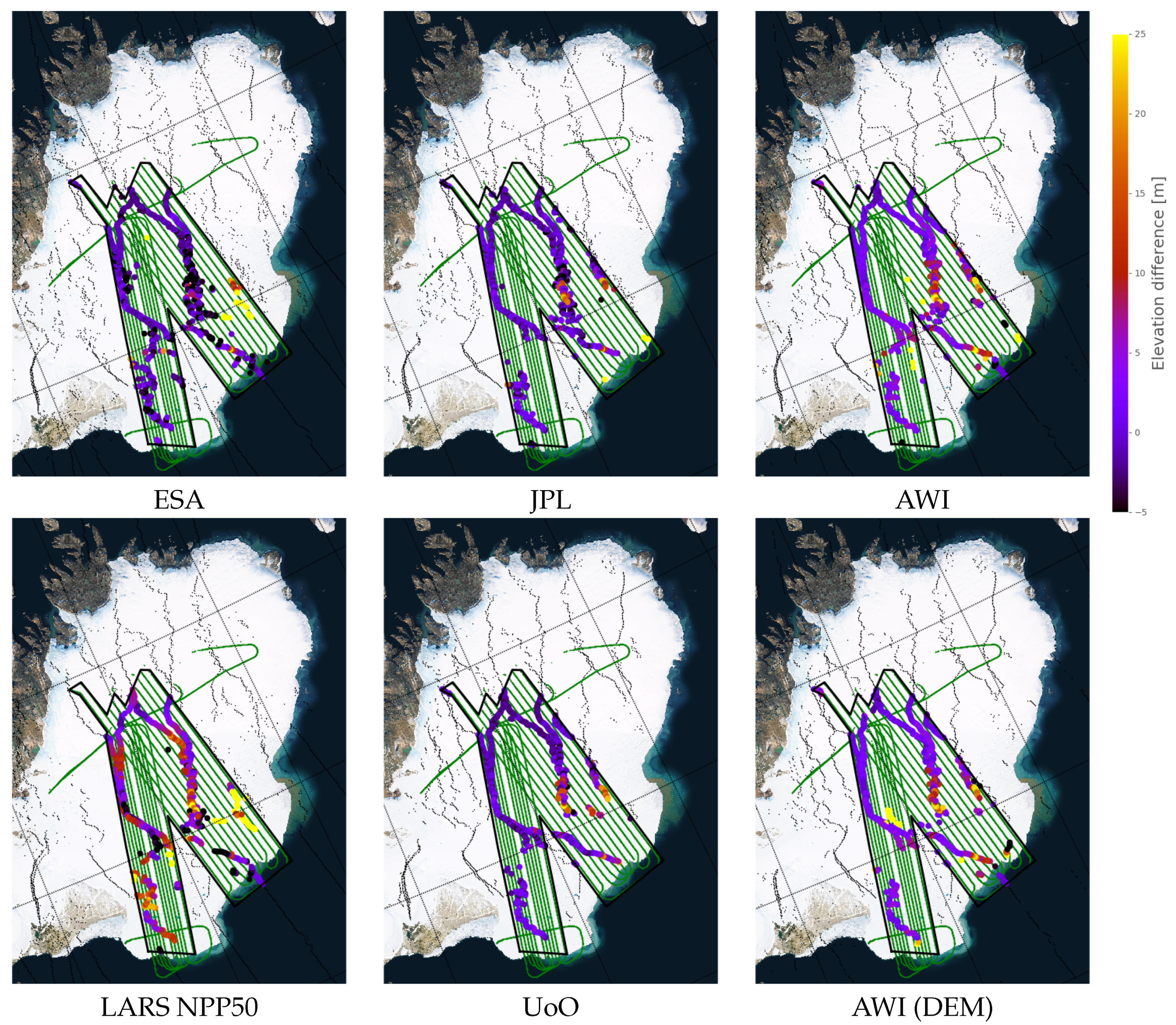
6. Results
Elevation differences (
) between the six CS2 L2 data sets and the surface elevations mapped with ALS are shown in
Figure 2. The CS2 data locations are indicated by black dots, and the polygon that marks the full interpolation area for the ALS data (Area 1) is shown by a black line.
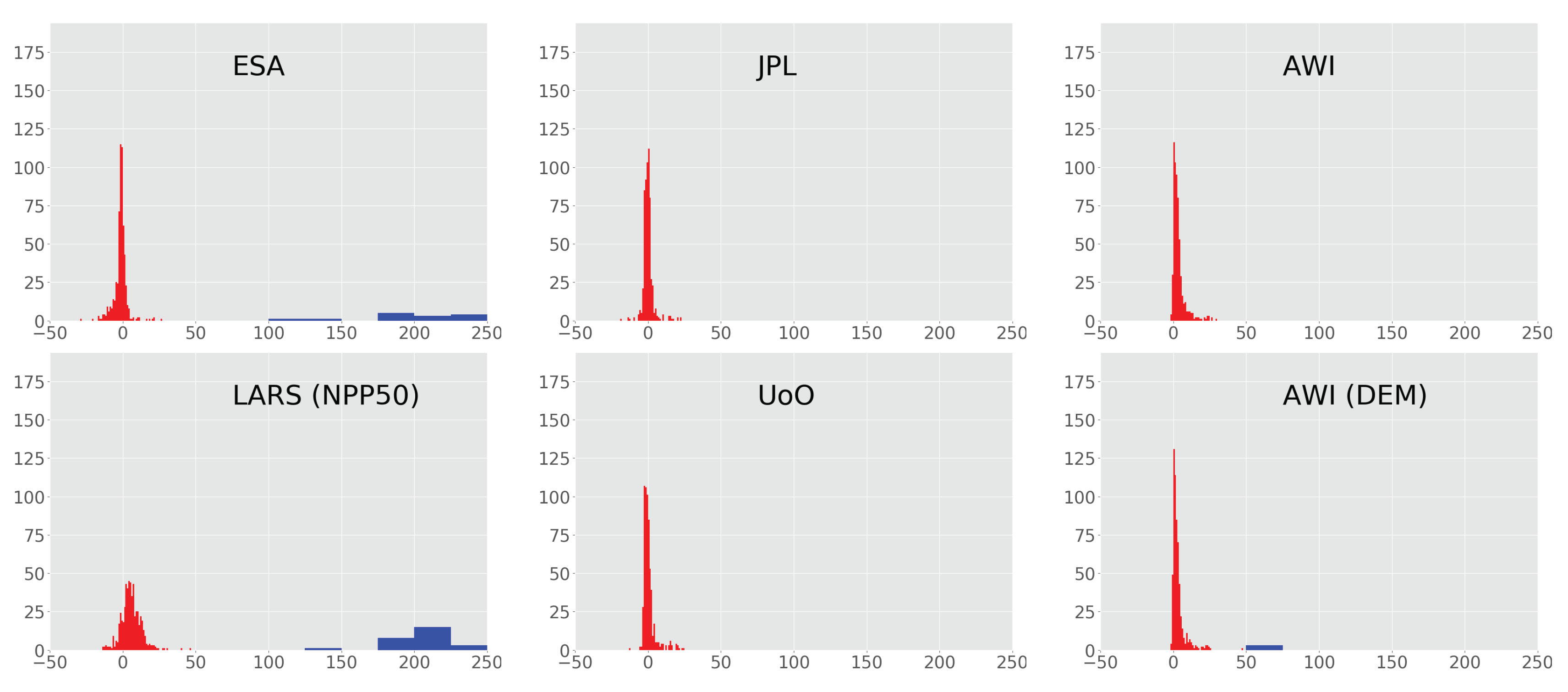
The histograms of the
estimates for all 600 common points for the six data sets are shown in
Figure 3. The range [−50 m, 50 m] of the
values in the histogram are given in bins of 1 m (shown in red), while for values outside this range, the bin size is 25 m (shown in blue). Only UoO did not have absolute differences larger than 50 m, whereas the others had 7, 16, 17, 6, and 40 for AWI, AWI (DEM), ESA, JPL, and LARS respectively.
The statistics of the derived
values from all six CS2 L2 data sets, described by their mean, median, and standard deviation, are given
Table 1. The statistics are based on all available
values for a given data set, and it is seen that the number of
values differed, which is a consequence of the different outlier detection strategies implemented in the individual processing chains. The AWI data set provided the most
values (828), while the JPL provided the fewest (725). The table also contains the statistics for only those
data points that had common nadir points in all six data sets (the numbers in parenthesis). Therefore, the main results shown in
Table 1 give the performance of each full data set, while the numbers in parentheses show the statistics which are best suited for a direct comparison of the performance of the processors. The absolute lowest values of mean, median, and standard deviation are highlighted in bold. From the full data set analysis (
Table 1) we see that the ESA data set provided a low mean value, but the largest standard deviation. We see from the statistics of the common data points (
Table 1) that the heights derived from the JPL SARIn processor generally agreed best with the ALS data, but that also the AWI and UoO processors provided results with good validation statistics. The ESA, JPL, and UoO data were the only data sets that yielded a negative median of
, indicating that the CS2 heights were generally lower than the ALS heights.
7. Discussion
From the spatial maps of the CS2-ALS elevation differences (
Figure 2), we can see more specifically where the different data sets’ performances are good and where they are degraded. In general, we see that all six data sets showed better agreement with the western-most ALS grid (area 2), compared to the eastern one (area 3). This is probably due to the more gentle topography in the Western region compared to the Eastern part. The latter covers a surging glacier [
35], and the surface here is characterized by rough topography with many deep crevasses, reflected in the standard deviation of area 3 (
Table 1). This rough terrain might be challenging for the processors, and in addition may not sample the topography accurately enough with a 2 km grid spacing. To avoid interpolating the ALS data, we attempted to derive statistics on only overlapping or closely separated ALS and CS2 data, but this resulted in a very small data set, which was not suitable for a robust validation.
Due to the nature of the CS2 SARIn measurements, the precise geolocation of the measurements is a very important part of a given processing chain. It is clear by visual inspection of the data that this procedure differed substantially between the processors considered here.
Figure 4 shows the large variability in the geolocations of CS2 measurements from the different L2 data sets. The figure shows both the locations of the derived heights (colors indicating different processors) as well as their nadir position (black). In the inset in the figure, we show for clarity the data locations for a single CS2 track. Here it is seen that along most of the track, the locations of the different data sets agreed well, but also that in specific regions individual processors seemed to struggle and produce locations that clearly deviated. For example in the southern end of the selected track, we see that the ESA echo locations deviated from the path of the other data sets. A correct geolocation is probably one of the most important parts of a successful SARIn processor, and this could be the focus of future studies. The AWI (DEM), JPL, and UoO processors had the best validation statistics, and common for these processors was a general good agreement of the echo-geolocation. Furthermore it is crucial to implement an appropriate retracker or threshold, as this alone has been shown to affect the performance over Greenland [
3]. Common for these three processing chains is the use of a reference DEM to guide the interferometric processing in order to avoid large outliers caused by 2
phase wrapping. This was shown by the reduced standard deviation of AWI (DEM) compared to AWI for areas 1 and 3.
Our analysis shows that, with the exceptions of ESA, JPL, and UoO data, the mean and median of
from the other processors (both complete and common data) were positive (
Table 1). This finding is surprising since, due to possible penetration of the radar signal into the snow [
36,
37] we would expect these to be negative (i.e., CS2 lower than ALS). The ALS data were averaged to 100 × 100 m resolution. In a heavily crevassed area such as area 3, this would result in a lower average surface, since the elevation originating from within the crevasses is included. Conversely, the CS2 radar altimeter measures the highest point in the footprint. This was confirmed by the positive
in area 3 and negative
in area 2 mapped by UoO. However, the other CS2-data showed results which cannot be explained by the presence of crevasses. At present, we do not have a good explanation for this finding, although one possible explanation could be the presence of a bias in the CS2 L1b data itself. The presence of a potential bias does not affect the conclusions drawn in this study, as it does not affect the standard deviations.
The criteria of using only CS2 data from the same month as the ALS data were collected should minimize any actual elevation differences between the two data sets caused by, for example, snow fall. However, such actual elevation changes cannot be eliminated completely. Any influence of actual surface elevation differences occurring between the time of the satellite and airborne measurement will affect the statistics, but since they are the same for all six data sets, the inter-comparison is still valid. Additionally, we investigated if a slope-dependent bias was present in the data but this was not the case.
It should be emphasized that the conclusions on the preferred processing scheme drawn in this study cannot be directly transferred to other locations, since climatology and snow characteristics might differ and this would likely have an impact on the performance of each processing strategy, as the radar altimetry data are heavily dependent on these parameters.
8. Conclusions
Data from six different CryoSat-2 SARIn processing chains (ESA, JPL, AWI DEM, AWI, LARS NPP50, UoO) were tested and compared through a comparison of their respective cross-over difference statistics with ALS data over the Austfonna ice cap collected in April 2016, during a dedicated ESA CryoSat-2 validation campaign. Our study shows that the heights derived from the AWI, JPL, and UoO SARIn processors agreed best with the ALS data. These processors were designed specifically for the land ice application, and all three identify and use analysis of the first significant leading edge, rather than using the entire waveform. We believe that the improved performance of these three processors is also related to the fact that the POCA is derived from only the leading edge and not the whole waveform. The LARS processors, which were designed for other purposes, provided the data sets which deviated most from the ALS validation data. For this reason, we found that dedicated land ice SARIn processing chains are needed to derive reliable height estimates. The major difference between the processing chains is in how data are geo-located, and this had a large impact on the validation statistics. The geo-location of the data is dependent on the retracker and phase filtering applied since these determine the look angle that dictates the across-track position of the measurement. Here, the preferred processing chains (AWI (DEM), UoO, and JPL) use a reference DEM to guide the interferometric processing to avoid large outliers caused by 2 phase wrapping.
As all presented data set and validation procedures are made available online, we see this study as a benchmark for future retracker development.
Supplementary Materials
The following are available online at
https://www.mdpi.com/2072-4292/10/9/1354/s1. All CS2 and ALS data are available in the supporting on-line material (SOM). The SOM also contains the Python code used to make the statistics, to allow future retracker developments to be directly benchmarked against this study.
Author Contributions
L.S.S. and S.B.S. conceived and designed the study based on the findings in the ESA CryoSat-2 Validation Land-ice project. S.B.S., V.H., J.N., L.S., and L.G. contributed with CryoSat-data; All authors contributed to writing the paper and discussed the results. H.S., L.S.S. and S.B.S. participated in ALS field campaign and processing; R.F. organized the overall field campaign logistics in 2016, along with M.W.J.D. as the acting ESA-officer.
Funding
This study was founded through ESA CryoSat land validation, contract 4000109790/13/NL/CT/ab. The German Ministry of Economics and Technology (grant 50EE1331 to V. Helm) has supported this work.
Conflicts of Interest
The authors declare no conflict of interest.
References
- Parrinello, T.; Shepherd, A.; Bouffard, J.; Badessi, S.; Casal, T.; Davidson, M.; Fornari, M.; Maestroni, E.; Scagliola, M. CryoSat: ESA’s I ce Mission—Eight Years in Space. Adv. Space Res. 2018, 62, 1178–1190. [Google Scholar] [CrossRef]
- Helm, V.; Humbert, A.; Miller, H. Elevation and elevation change of Greenland and Antarctica derived from CryoSat-2. Cryosphere 2014, 8, 1539–1559. [Google Scholar] [CrossRef] [Green Version]
- Nilsson, J.; Gardner, A.; Sørensen, L.S.; Forsberg, R. Improved retrieval of land ice topography from CryoSat-2 data and its impact for volume-change estimation of the Greenland Ice Sheet. Cryosphere 2016, 10, 2953–2969. [Google Scholar] [CrossRef]
- Mcmillan, M.; Leeson, A.; Shepherd, A.; Briggs, K.; Armitage, T.W.K.; Hogg, A.; Kuipers Munneke, P.; Broeke, M.; Noel, B.; Berg, W.J.; et al. A high resolution record of Greenland mass balance. Geophys. Res. Lett. 2016, 43, 7002–7010. [Google Scholar] [CrossRef]
- Simonsen, S.B.; Sørensen, L.S. Implications of changing scattering properties on Greenland ice sheet volume change from Cryosat-2 altimetry. Remote Sens. Environ. 2017, 190, 207–216. [Google Scholar] [CrossRef]
- McMillan, M.; Shepherd, A.; Sundal, A.; Briggs, K.; Muir, A.; Ridout, A.; Hogg, A.; Wingham, D. Increased ice losses from Antarctica detected by CryoSat-2. Geophys. Res. Lett. 2014, 41, 3899–3905. [Google Scholar] [CrossRef] [Green Version]
- Foresta, L.; Gourmelen, N.; Palsson, F.; Nienow, P.; Björnsson, H.; Shepherd, A. Surface elevation change and mass balance of Icelandic ice caps derived from swath mode CryoSat-2 altimetry. Geophys. Res. Lett. 2016, 43, 12138–12145. [Google Scholar] [CrossRef]
- Gray, L.; Burgess, D.; Copland, L.; Demuth, M.N.; Dunse, T.; Langley, K.; Schuler, T.V. CryoSat-2 delivers monthly and inter-annual surface elevation change for Arctic ice caps. Cryosphere 2015, 9, 2821–2865. [Google Scholar] [CrossRef]
- Laxon, S.W.; Giles, K.A.; Ridout, A.L.; Wingham, D.J.; Willatt, R.; Cullen, R.; Kwok, R.; Schweiger, A.; Zhang, J.; Haas, C.; et al. CryoSat-2 estimates of Arctic sea ice thickness and volume. Geophys. Res. Lett. 2013, 40, 732–737. [Google Scholar] [CrossRef] [Green Version]
- Ricker, R.; Hendricks, S.; Helm, V.; Skourup, H.; Davidson, M. Sensitivity of CryoSat-2 Arctic sea-ice freeboard and thickness on radar-waveform interpretation. Cryosphere 2014, 8, 1607–1622. [Google Scholar] [CrossRef] [Green Version]
- Kwok, R.; Cunningham, G.F. Variability of Arctic sea ice thickness and volume from CryoSat-2. Philos. Trans. R. Soc. A 2015, 373, 20140157. [Google Scholar] [CrossRef] [PubMed] [Green Version]
- Tilling, R.L.; Ridout, A.; Shepherd, A. Near Real Time Arctic sea ice thickness and volume from CryoSat-2. Cryosphere 2016, 10, 2003–2012. [Google Scholar] [CrossRef]
- Nielsen, K.; Stenseng, L.; Andersen, O.B.; Villadsen, H.; Knudsen, P. Validation of CryoSat-2 SAR mode based lake levels. Remote Sens. Environ. 2015, 171, 162–170. [Google Scholar] [CrossRef] [Green Version]
- Villadsen, H.; Deng, X.; Andersen, O.B.; Stenseng, L.; Nielsen, K.; Knudsen, P. Improved inland water levels from SAR altimetry using novel empirical and physical retrackers. J. Hydrol. 2016, 537, 234–247. [Google Scholar] [CrossRef] [Green Version]
- Jiang, L.; Nielsen, K.; Andersen, O.B.; Bauer-gottwein, P. Monitoring recent lake level variations on the Tibetan Plateau using CryoSat-2 SARIn mode data. J. Hydrol. 2017, 544, 109–124. [Google Scholar] [CrossRef]
- Armitage, T.W.K.; Bacon, S.; Ridout, A.L.; Thomas, S.F.; Aksenov, Y.; Wingham, D.J. Arctic sea surface height variability and change from satellite radar altimetry and GRACE, 2003–2014. J. Geophys. Res. Oceans 2016, 121, 4303–4322. [Google Scholar] [CrossRef]
- CSAG. CryoSat Calibration & Validiation Concept; Technical Report November, ESA/CPOM; Centre for Polar Observation & Modelling Department of Space & Climate Physics, University College London: London, UK, 2001. [Google Scholar]
- Skourup, H.; Simonsen, S.B.; Sørensen, L.S.; Bella, A.D.; Forsberg, R.; Hvidegaard, S.M.; Helm, V. ESA CryoVEx/EU ICE-ARC 2016—Airborne Field Campaign with ASIRAS Radar and Laser Scanner over Austfonna, Fram Strait and the Wandel Sea; Technical Report; National Space Institute, Technical University of Denmark: Kgs. Lyngby, Denmark, 2017. [Google Scholar]
- Moholdt, G.; Kääb, A. A new DEM of the Austfonna ice cap by combining differential SAR interferometry with icesat laser altimetry. Polar Res. 2012, 31, 18460. [Google Scholar] [CrossRef] [Green Version]
- Hagen, J.O.; Liestol, O.; Roland, E.; Jorgensen, T. Glacier Atlas of Svalbard and Jan Mayen; Norwegian Polar Institute: Tromsø, Norway, 1993; pp. 1–143. [Google Scholar]
- Dunse, T.; Schuler, T.V.; Hagen, J.O.; Eiken, T.; Brandt, O.; Hogda, K.A. Recent fluctuations in the extent of the firn area of Austfonna, Svalbard, inferred from GPR. Ann. Glaciol. 2009, 50, 155–162. [Google Scholar] [CrossRef] [Green Version]
- Schuler, T.V.; Dunse, T.; Østby, T.I.; Hagen, J.O. Meteorological conditions on an Arctic ice cap-8years of automatic weather station data from Austfonna, Svalbard. Int. J. Climatol. 2014, 34, 2047–2058. [Google Scholar] [CrossRef]
- Mavrocordatos, C.; Attema, E.; Davidson, M.W.J.; Lentz, H.; Nixdorf, U. Development of ASIRAS (airborne SAR/Interferometric altimeter system). In Proceedings of the 2004 IEEE International Geoscience and Remote Sensing Symposium (IGARSS’04), Anchorage, AK, USA, 20–24 September 2004; pp. 2465–2467. [Google Scholar]
- CRYOSAT Ground Segment Instrument Processing Facility—L2 Products Format Specification Baseline C. Available online: https://earth.esa.int/web/guest/missions/cryosat/unavailability-periods/-/article/cryosat-ground-segment-instrument-processing-facility-l2-l2-products-format-specification-l2-fmt-6636 (accessed on 19 July 2018).
- Gray, L.; Burgess, D.; Copland, L.; Dunse, T.; Langley, K.; Moholdt, G. A revised calibration of the interferometric mode of the CryoSat-2 radar altimeter improves ice height and height change measurements in western Greenland. Cryosphere 2017, 11, 1041–1058. [Google Scholar] [CrossRef]
- Scagliola, M.; Fornari, M.; Bouffard, J.; Parrinello, T. The CryoSat interferometer: End-to-end calibration and achievable performance. Adv. Space Res. 2017, 62, 1516–1525. [Google Scholar] [CrossRef]
- Wingham, D.J.; Francis, C.R.; Baker, S.; Bouzinac, C.; Brockley, D.; Cullen, R.; de Chateau-Thierry, P.; Laxon, S.W.; Mallow, U.; Mavrocordatos, C.; et al. CryoSat: A mission to determine the fluctuations in Earth’s land and marine ice fields. Adv. Space Res. 2006, 37, 841–871. [Google Scholar] [CrossRef]
- Stenseng, L.; Andersen, O.B. Preliminary gravity recovery from CryoSat-2 data in the Baffin Bay. Adv. Space Res. 2012, 50, 1158–1163. [Google Scholar] [CrossRef]
- Martin-Puig, C.; Ruffini, G.; Marquez, J.; Cotton, D.; Srokosz, M.; Challenor, P.; Raney, K.; rome Benveniste, J. Theoretical Model of SAR Altimeter over Water Surfaces. In Proceedings of the 2008 IEEE International Geoscience and Remote Sensing Symposium (IGARSS 2008), Boston, MA, USA, 7–11 July 2008. [Google Scholar]
- Jain, M.; Martin-Puig, C.; Andersen, O.B.; Stenseng, L.; Dall, J. Evaluation of SAMOSA3 adapted retracker using Cryosat-2 SAR altimetry data over the Arctic ocean. In Proceedings of the International Geoscience and Remote Sensing Symposium (IGARSS), Quebec City, QC, Canada, 13–18 July 2014; pp. 5115–5118. [Google Scholar]
- Jain, M.; Andersen, O.B.; Dall, J.; Stenseng, L. Sea surface height determination in the Arctic using Cryosat-2 SAR data from primary peak empirical retrackers. Adv. Space Res. 2015, 55, 40–50. [Google Scholar] [CrossRef]
- Abulaitijiang, A.; Andersen, O.B.; Stenseng, L. Coastal sea level from inland CryoSat-2 interferometric SAR altimetry. Geophys. Res. Lett. 2015, 42, 1841–1847. [Google Scholar] [CrossRef] [Green Version]
- Bao, L.; Lu, Y.; Wang, Y. Improved retracking algorithm for oceanic altimeter waveforms. Prog. Nat. Sci. 2009, 19, 195–203. [Google Scholar] [CrossRef]
- Armitage, T.W.K.; Wingham, D.J.; Ridout, A.L. Meteorological origin of the static crossover pattern present in low-resolution-mode CryoSat-2 data over central Antarctica. IEEE Geosci. Remote Sens. Lett. 2014, 11, 1295–1299. [Google Scholar] [CrossRef]
- Dunse, T.; Schellenberger, T.; Hagen, J.O.; Kääb, A.; Schuler, T.V.; Reijmer, C.H. Glacier-surge mechanisms promoted by a hydro-thermodynamic feedback to summer melt. Cryosphere 2015, 9, 197–215. [Google Scholar] [CrossRef]
- Rémy, F.; Flament, T.; Michel, A.; Blumstein, D. Envisat and SARAL/AltiKa Observations of the Antarctic Ice Sheet: A Comparison Between the Ku-band and Ka-band. Mar. Geod. 2015, 38, 510–521. [Google Scholar] [CrossRef]
- Nilsson, J.; Vallelonga, P.; Simonsen, S.B.; Sørensen, L.S.; Forsberg, R.; Dahl-Jensen, D.; Hirabayashi, M.; Goto-Azuma, K.; Hvidberg, C.S.; Kjaer, H.A.; et al. Greenland 2012 melt event effects on CryoSat-2 radar altimetry. Geophys. Res. Lett. 2015, 42, 3919–3926. [Google Scholar] [CrossRef] [Green Version]
© 2018 by the authors. Licensee MDPI, Basel, Switzerland. This article is an open access article distributed under the terms and conditions of the Creative Commons Attribution (CC BY) license (http://creativecommons.org/licenses/by/4.0/).

 ,
, 


