Automated Stone Detection on Side-Scan Sonar Mosaics Using Haar-Like Features


1
Wadden Sea Research Station, Helmholtz Centre for Polar and Marine Research, Alfred Wegener Institute, Hafenstraße 43, 25992 List, Germany
2
Leibniz Institute for Baltic Sea Research Warnemünde, Seestrasse 15, 18119 Rostock, Germany
*
Author to whom correspondence should be addressed.
Geosciences 2019, 9(5), 216; https://doi.org/10.3390/geosciences9050216
Submission received: 28 March 2019
/
Revised: 6 May 2019
/
Accepted: 7 May 2019
/
Published: 11 May 2019
(This article belongs to the Special Issue Geological Seafloor Mapping)
Abstract
:Stony grounds form important habitats in the marine environment, especially for sessile benthic organisms. For the purpose of habitat demarcation and monitoring, knowledge of the position and abundance of individual stones is necessary. This is especially the case in areas with a scattered occurrence of stones in an environment which is otherwise characterized by relatively mobile sandy sediments. Exposed stones can be detected using side-scan sonar (SSS) data. However, apart from laborious manual identification, there is as yet no automated or semi-automated method available for a fast and spatially resolved detection of stones. In this study, a Haar-like feature detector was trained to identify individual stones on an SSS mosaic (~12 km2) showing heterogeneous sediment distribution. The results of this method were compared with those of manually derived stones. Our study shows that the Haar-like feature detector was able to detect up to 62% of the overall occurrence of stones within the study area. Even though the sheer number of correctly identified stones was influenced by, e.g., the type of sediments and the number of grey values of the mosaic, Haar-like feature detectors provide a relatively easy and fast method to identify stones on SSS mosaics when compared to the manual investigation.
1. Introduction
Hard substrates, composed of, e.g., cobbles, boulders and bedrock, provide an essential habitat for a variety of both marine sessile and mobile species [1,2]. The functioning of these marine habitats is, however, threatened by both natural (e.g., sediment mobility) and anthropogenic pressure (e.g., fishing, aggregate extraction and construction of offshore windfarms) [3,4,5]. To preserve and support these habitats and the associated valuable ecosystem services, an efficient monitoring of these habitats is mandatory. This is especially important in areas where hard substrates are rare, e.g., in the sand-dominated North Sea.
The demarcation and monitoring of the condition of hard-substrate habitats need to consider substrate availability besides the investigation of the epibenthic assemblages. This is due to the strong dependency of sessile organisms on suitable anchor points. Various consolidated objects, both natural and artificial (e.g., stones, mussel accumulations, shipwrecks, pipelines or construction basements), can provide shelter and substrate for a variety of sessile and mobile species (e.g., [6,7,8]). The sediment composition of the seafloor has a strong influence on the availability of such substrates. In environments with high sediment mobility, e.g., shallow shelf seas affected by waves and tides, hard substrates might become temporarily buried while previously buried ones might become exposed [9,10]. As yet, the spatial detection of underwater objects can only be achieved using hydroacoustic remote-sensing devices such as side-scan sonars (SSS), multibeam echo sounders (MBES), and parametric sediment echo sounders (pSES) (e.g., [11,12,13]). SSS data are usually analyzed by means of automated and semi-automated methods for the detection of objects such as ship wrecks or mines (e.g., [14,15]). Objects which protrude from the seafloor can be identified in SSS data as they cause a signal of strong backscatter followed by a weak backscatter (acoustic shadow) perpendicular to the moving SSS. This pattern can be more or less clear as a function of the quality and resolution of the SSS data, the size and the material composition of the object, and the acoustic reflectivity of the seafloor. However, even though many objects are visually clearly identifiable, the automated counting, extraction and localization of individual objects for further applications remains difficult to impossible. Several statistical and machine learning algorithms were developed to support the automated identification and extraction of areas and objects. These focused on differences between pixel intensities, e.g., eCognition in [16], Viola–Jones Cascade [17], wavelet analysis [18], Back Propagation and Convolutional Neural Networks ([19,20,21] and references therein), among other approaches.
The training and application of so called Haar-like feature detectors was shown to produce promising results in a variety of different disciplines to detect objects on images (e.g., face detection, vehicle detection and the detection of mine-like objects on SSS mosaics) [15,22]. As yet, it is not known whether this method is also suitable for the spatial detection of hard substrates.
Just recently, the German Federal Agency for Nature Conservation (BfN) proposed a mapping guideline to demarcate reefs in the North and Baltic Sea [23]. According to this guideline, the demarcation of reefs in the North Sea should be based on SSS data, which were acquired with a frequency of ≥300 kHz and a resolution suitable to detect stones ≥ 30–50 cm of diameter. It is based on a four-step approach, which follows the observer-based tagging of stones, which is, however, a very tedious and time-consuming process suitable only for very small areas.
To underpin this approach, the aim of this study was (1) to train a Haar-like classifier to detect individual objects on a large SSS mosaic, (2) to estimate the performance of the detector with respect to different sediment types, detection thresholds and number of grey values of the tested mosaic, and (3) to propose a spatial demarcation of reefs of a study site in the German Bight based on the mapping guideline [23].
2. Material and Methods
2.1. Study Site and SSS Data
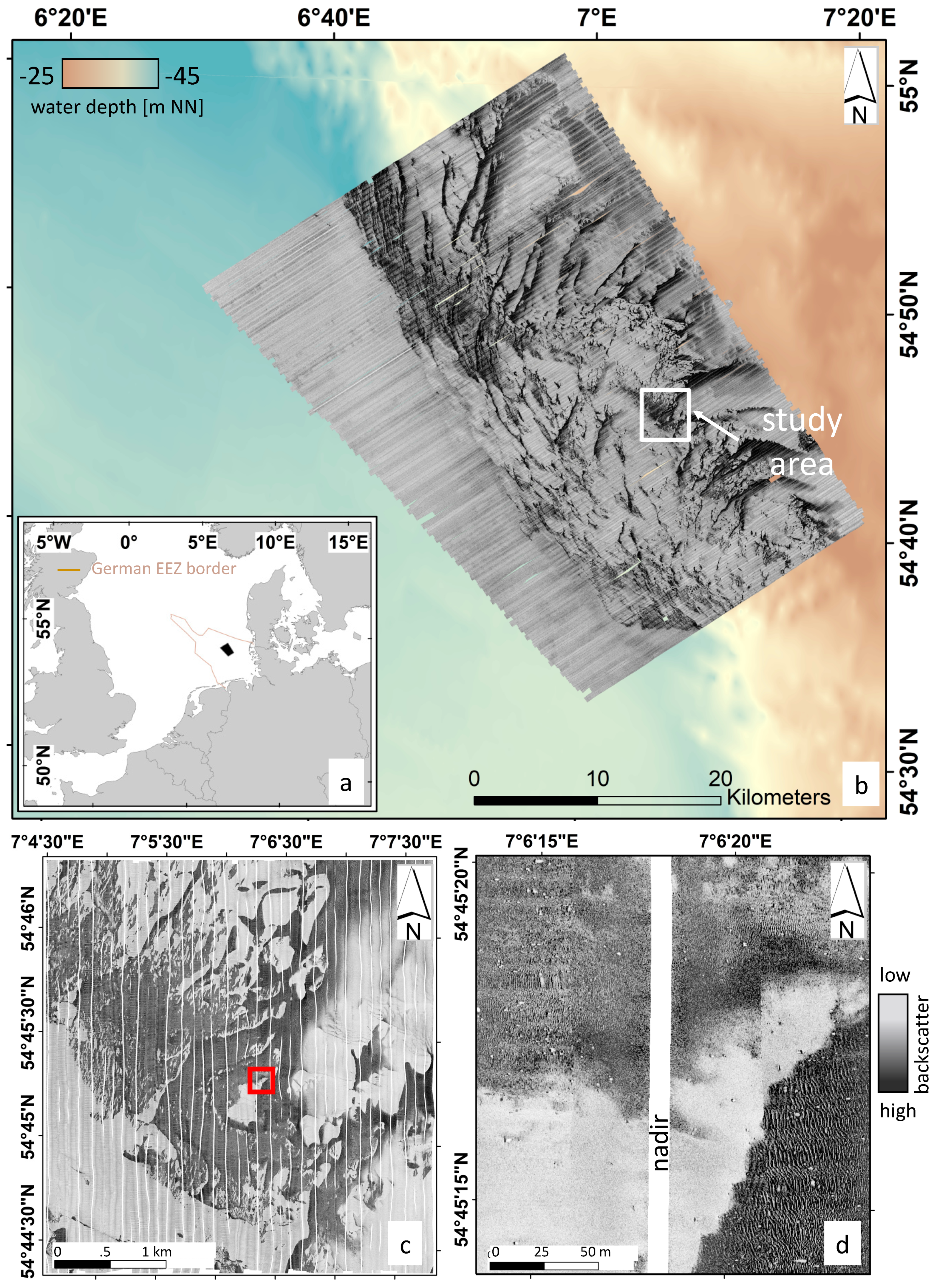
The study site is located within the Sylt Outer Reef (SOR), approximately 40 nautical miles west of the Island Sylt in the German Bight, SE North Sea, and has a size of ~12 km2 (Figure 1). The SOR is a massive submarine moraine ridge with glacial till and meltwater deposits that formed during the Saalian glacial (MIS 6) [24]. Water depths in the area are between 30 and 40 m. The modern seafloor in the study area is composed of a patchy distribution of fine to coarse sands, with gravels, cobbles and boulders emerging from the seafloor [13,25]. Most of these hard substrates are colonized by epifauna [8]. Since 2017, the SOR is protected as a Special Area of Conservation (SAC) according to the European Union’s Habitats Directive (92/43/EEC). It includes the habitat types ‘sandbanks’ (Annex 1 EUNIS habitat type: code 1110) and ‘reefs’ (Annex 1 EUNIS habitat type code: 1170).
SSS data were collected using a towed multi-pulse Edgetech 4200-MP during a survey in October 2016. The SSS was operated with a frequency of 300 kHz. The speed of the ship was approximately 5 knots, and the range was set to 75 m to achieve an along track resolution of at least 0.25 m. The SSS raw data were processed including slant range correction, speed, layback and gain normalization using SonarWiz (Chesapeake Technology, California, CA, USA). The nadir line was cut out to 5 m both in port- and starboard direction to reduce the noise of the resultant mosaic.
To investigate the sizes of the stones within the study area, a subsample of randomly chosen stones was measured on the waterfall mode of the SSS. The sizes were manually obtained with the target logger of the EdgeTech Discover software (4200-MP, version 7.00) by measuring the length of the acoustic shadow.
2.2. Training and Application of the Detector
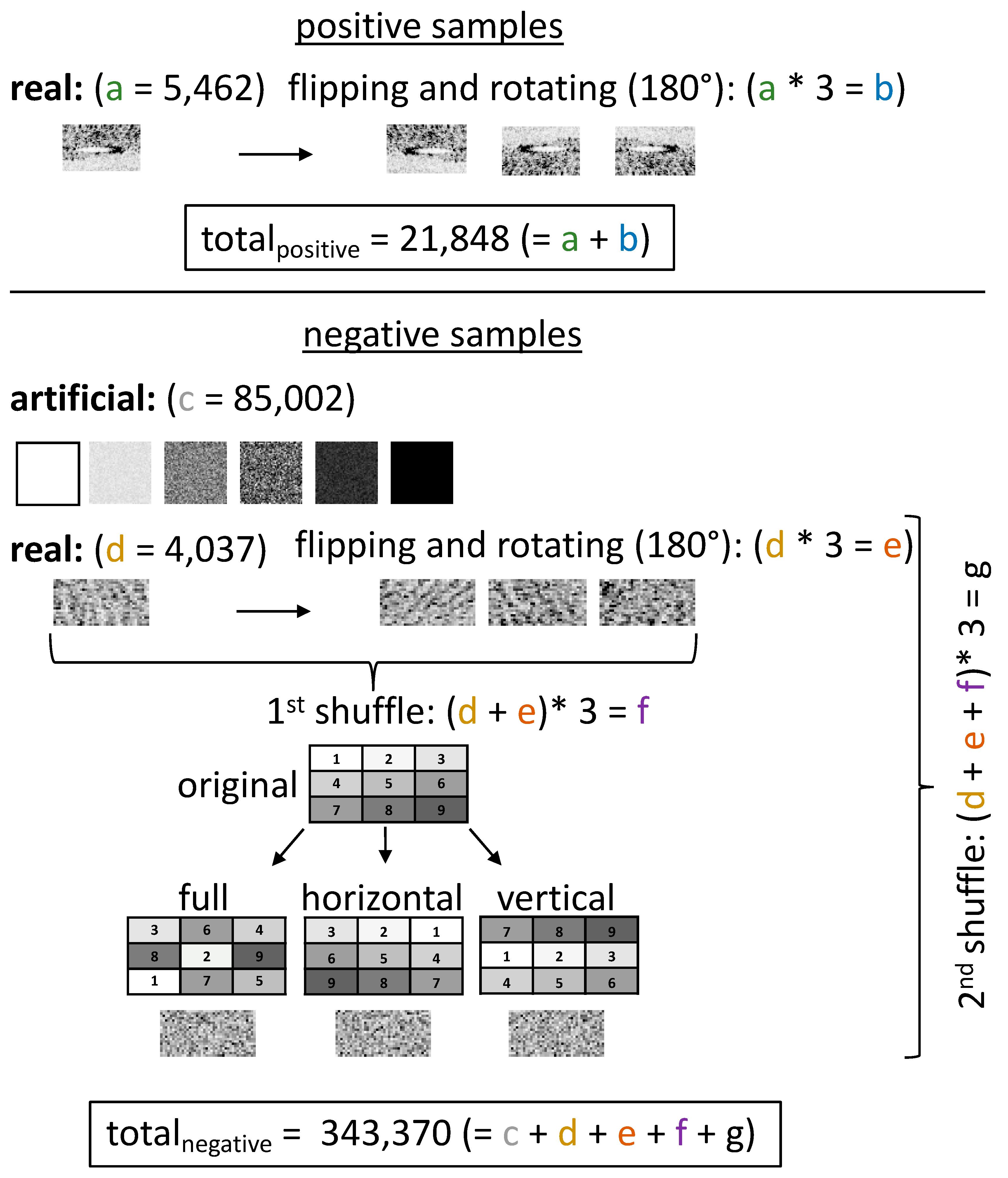
The training of a Haar-like feature detector requires a large amount (many thousands) of positive (= matching) and negative (= not matching) images of the object in question (e.g., [27]). In order to obtain this, raw SSS data of multiple stony areas of the Sylt Outer Reef were replayed in the waterfall mode (displayed in 256 grey values) and automatically transformed into still images using the Edgetech Discover 4200-MP software (version 7.00). The still images were imported into Matlab’s (MathWorks R2018b, Natick, MA, USA) Image Labeler application (part of Matlab’s Computer Vision System Toolbox) and positive samples (i.e., a backscatter pattern that indicates a stone) were manually extracted. Rectangles were drawn around the stones including some backscatter information of the surrounding background (average width = 44 ± 11 pixels, average height = 20 ± 6 pixels). These are the ‘real positive samples’. ‘Real negative samples’ were generated from those SSS still images that did not contain any stone by cutting out sub-images in the size of 40 × 20 pixels (Figure 2).
To enlarge the training dataset, further ‘artificial negative samples’ were created by producing images (here with a size of 100 × 100 pixels) composed of randomly assigned grey values using Matlab. The creation and implementation of artificial images in the training procedure is a common method to improve the performance of a detector (e.g., [15]). Therefore, all real positive and negative samples were quadrupled by flipping and rotating the images by 180 degrees (cf. Figure 2). To achieve a further increase in the number of negative samples, the pixel values of each image retrieved from real samples were randomized as well as shuffled in their horizontal and vertical direction. This pixel-randomization procedure was repeated a second time using the previously created dataset. This procedure increased the number of real negative images by a factor of 64. In total, 21,848 positive and 343,370 negative samples were available for the training of the detector.
The Haar-like feature detector was trained using the cascaded object detector integrated in Matlab’s Computer Vision System Toolbox. The following settings were used: false alarm rate: 0.1; true positive rate: 0.995; number of cascade stages: 29; object training size in pixels: height = 10, width = 15; negative samples factor: 2. The false alarm rate defines the acceptable fraction of negative samples per stage, which are incorrectly classified as positive samples. The true positive rate is the minimum fraction of correctly classified positive samples.
The trained Haar-like feature detector was applied on the SSS mosaic with a minimum detector size of 10 × 15 pixels and a maximum detector size of 30 × 30 pixels. These values were manually determined as they were found to give the best detection results with respect to the size of the stones in the SSS mosaic. To assess the influence of the merging threshold level of the detector and the number of grey values of the SSS mosaic on the resulting detections, the thresholds were set to 6, 8, 10, 12 and 20, respectively, and the number of grey values of the SSS mosaic were set to 32, 64, 128, 192 and 256, respectively. The merging threshold level of the detector is a tunable integer that helps to reduce false detections. To pass a higher threshold level, individual objects must be detected multiple times during the multiscale detection phase. The coordinates of the center points of each resulting bounding box (i.e., the detected objects) of all threshold and grey value combinations were extracted and used for the subsequent analysis in ArcGIS (Esri, Redlands, California, USA).
2.3. Evaluation of the Performance
The performance of the detector was evaluated by comparing the results of the detector (further referred to as automatic method) with the results of manually tagged stones. Manually tagged stones were derived from SSS files that were replayed in the waterfall mode and the selection of obvious stones using the target logger. The evaluation was done with respect to the total number of spatially matching detections. It was further done by evaluating the number of matches with respect to four different seafloor types, and the size of a resulting reef area based on the method provided by the [23] (both described in the following).
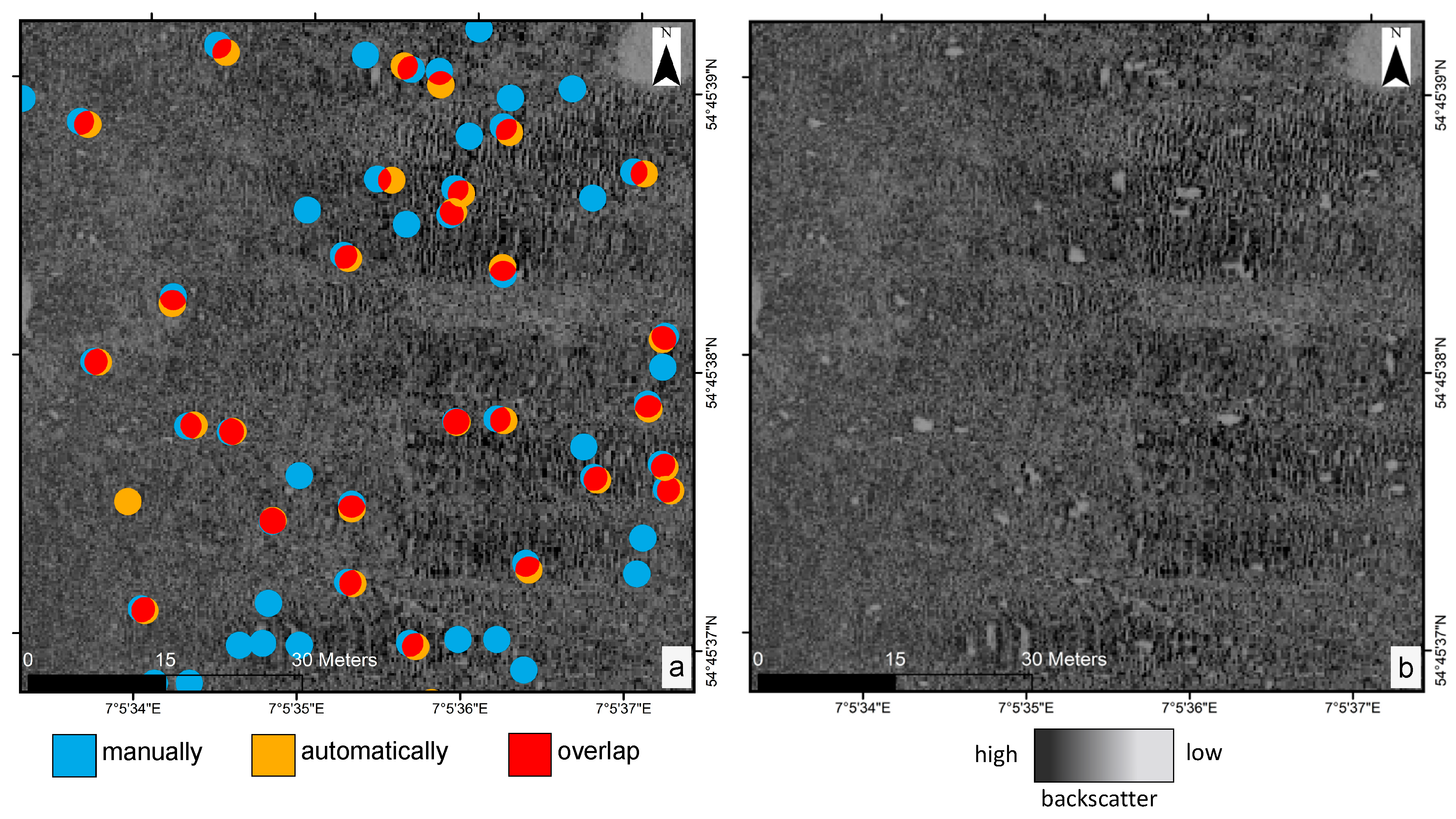
The comparison of the total number of spatial matches was evaluated by drawing buffers around each automatically and manually detected stone using diameters of 1.50 and 3.00 m, respectively. This approach was based on the observed offset of the positioning of point features derived from manually and automatically detected stones. The mismatch was triggered by the different-sized bounding boxes of the detector to identify different sizes of stones and the non-standardized marking of stones during the manual detection procedure. Those buffers that overlap, or rather have the largest overlap in the case of multiple overlaps, were supposed to represent the same stone and counted as one match (Figure 3). Each detected stone was only allowed to be counted once.
The influence of different backscatter intensities, which represent different seafloor types, on the performance of the detector was assessed by the manual classification and interpretation of the backscatter intensities of 25 × 25 m grid cells. The four categories used were (1) fine sand areas showing a comparatively weak and homogeneous backscatter, (2) rippled sediments, (3) stony grounds with a comparatively strong backscatter, and (4) areas with a mixed occurrence of the above-mentioned sediment types. Again, overlapping buffers of automatically and manually detected stones with buffer diameters of 1.50 and 3.00 m were assumed to be matching stones.
The reef areas were demarcated according to the mapping guideline developed by [23]: The demarcation of the geogenic reef type ‘stonefield/boulderfield North Sea’ is based on a four-step approach: (1) a buffer of 75 m is drawn around every individual stone (≥ approx. 30–50 cm), (2) stones, whose buffers overlap are classified as an ‘accumulation of stones and boulders’ and (3) form a ‘geogenic reef’ if the accumulation contains ≥21 individual stones, which have an average distance of ≤50 m to their nearest neighbors. Areas, which do not contain stones but are surrounded by ‘geogenic reefs’ are included in this category (4). All analyses were realized using ESRI’s ArcGIS 10.4 (ESRI, Redland, CA, USA).
To identify the best threshold and grey-value combination of the detector and the mosaic (see Section 2.2) Equation (1) was developed and used as a decision support (DS):
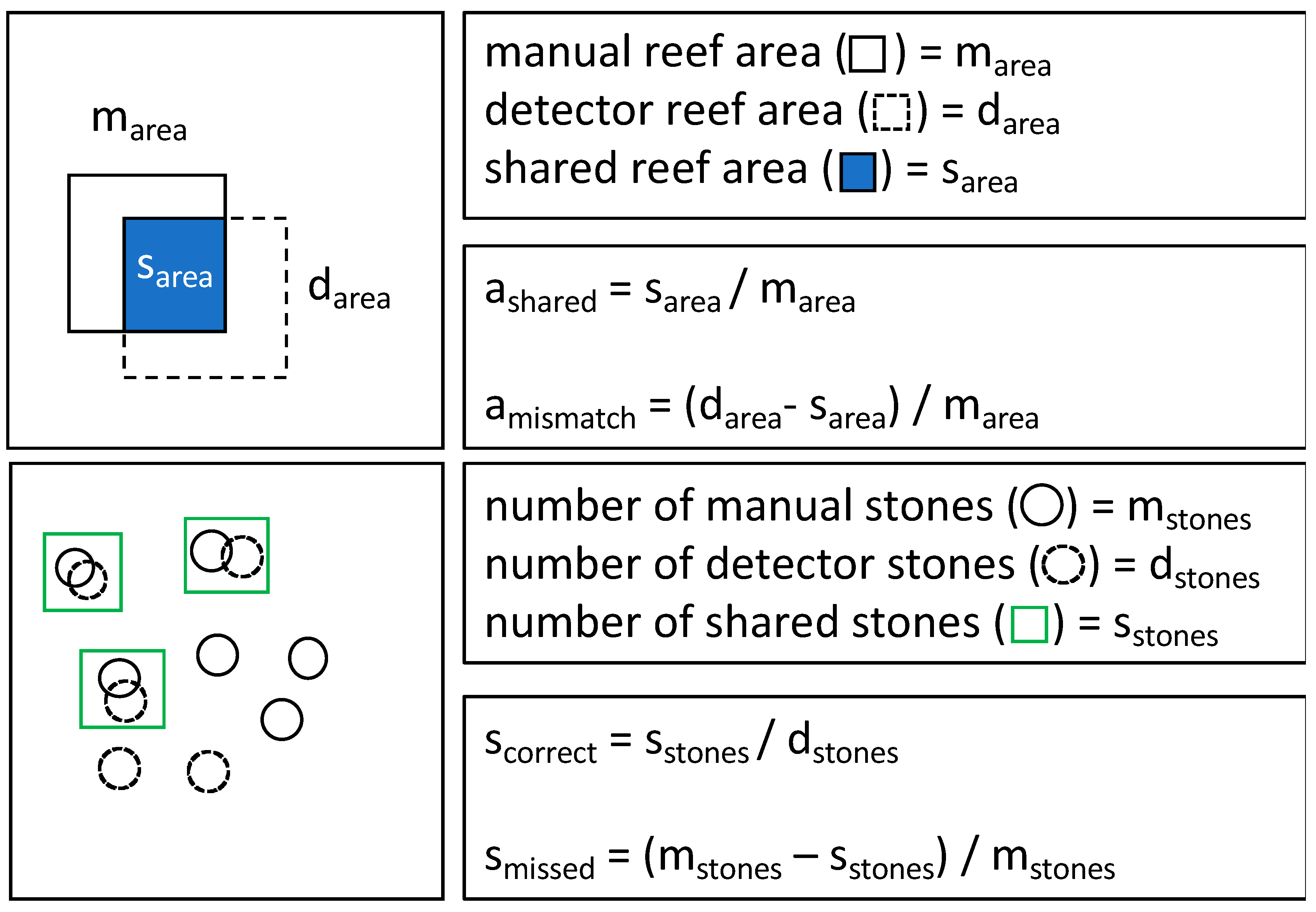
The first part of the equation includes the size of the calculated reef area [km2] derived from the detector () multiplied by the factor (range: 0–1) (Figure 4). This factor corresponds to the proportion of the reef area shared () with the reef area derived from manually tagged stones () with 1 meaning that the two reef areas completely overlap. The factor stands for the proportion of the calculated reef area that is not shared with the manual method (i.e., lies outside of it). It is based on the reef area derived from the automated method that is not shared with the area derived from the manual method. The second part of the equation is based on the number of stones derived from the detector (). The factor (range: 0–1) corresponds to the proportion of correctly identified stones () with regard to the total number of automatically identified stones () with 1 meaning that all detected stones are correctly identified. The proportion of the number of missed stones derived from the automated method and the total number of manually tagged stones () is described by the factor . The exponents and can be either set to 1 or 2, respectively, to provide an additional weight to either the correctly assigned reef area or the number of stones. The threshold and grey-value combination that produces results closer to retrieved from the manual method is assumed to perform best.
2.4. Statistical Analyses
A one-way analyses of variance (ANOVA) and a Bartlett’s test for equal variances was performed to test for statistically significant differences between the proportion of correctly identified stones and different sediment types. For this test, the proportion of correctly identified stones was pooled for the different threshold and grey values. A Tukey–Kramer post-hoc test was used to identify statistically significant differences between the groups. Two-sample t-tests were used to evaluate the differences of the proportion of correctly identified stones for the different sediment types and the two buffer sizes (1.50 and 3.00 m).
3. Results
3.1. Number of Detections
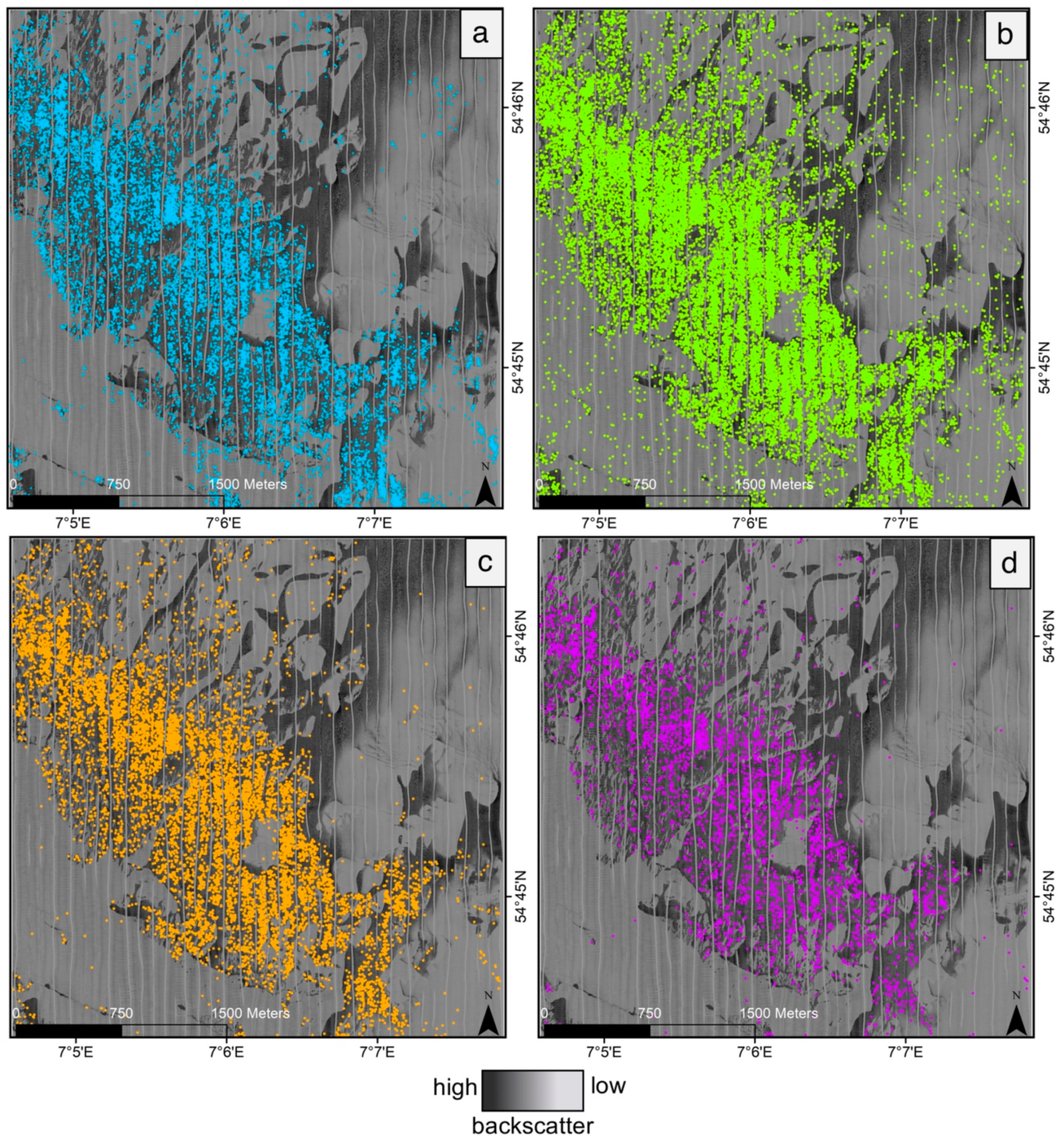
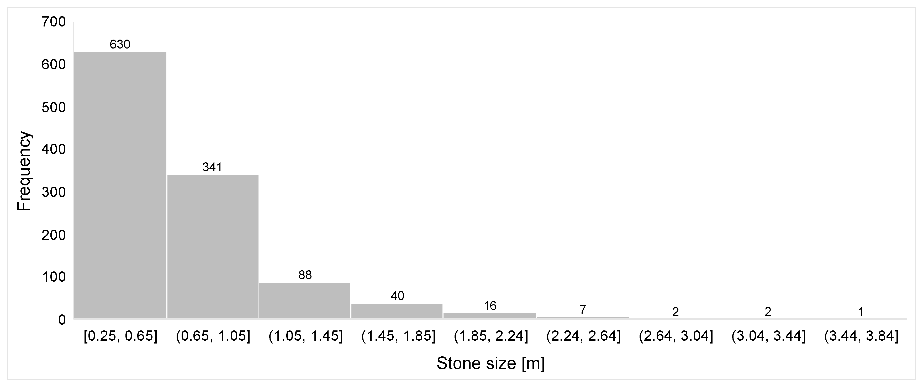
In total, 12,852 stones were manually tagged on the SSS mosaic (Figure 5a). They were mostly aligned in an area stretching from the north-western to the south-eastern part with an average Euclidian distance of 9.00 m to the nearest neighbor. This average distance is an important parameter to assess the density of stones within an area. The average size of the stones was 0.72 ± 0.40 m with the highest frequency in the range of 0.25–0.65 m and only a few stones were larger than 2.00 m (Figure 6).
Table 1 shows the absolute amount of detections and the average Euclidian distance to the nearest neighbor of automatic detections as a function of the threshold value of the detector and the number of grey values of the SSS mosaic. The number of detections generally decreased with an increasing threshold value, while the average Euclidian distance increased. The highest number of detections was 21,118, observed for the SSS mosaic displayed with 64 grey values and a threshold value of 6, while the lowest number was 1544 with 32 grey values and a threshold value of 20.
3.2. Accuracy of Predicted Stone Numbers
The concordance of the automatic detections with the manually tagged stones is shown in Table 2 and Table 3 for buffer sizes of 1.50 and 3.00 m, respectively (see Section 2.3). Again, the number of matching stones decreased with an increasing threshold value of the detector. The highest number of concordant stones was 7919, found for the SSS mosaic displayed with 64 grey values and a threshold of 6 at a buffer size of 3.00 m. The proportion to the total number of automatically detected stones (37%) was, however, continuously lower when compared to the other grey value and threshold combinations. In general, the buffer size of 3.00 m revealed a higher number of matching stones throughout the different grey value and threshold combinations. Here, the proportion of the concordant stones to the total number of automatically detected stones increased by up to 5% when compared to the buffer size of 1.50 m. The observed differences between the grey values 128, 192 and 256 were only marginal.
The proportion of correctly detected stones from the automatic method and the total number of manually tagged stones is presented in Table 4 for buffer sizes of 1.50 and 3.00 m. The highest proportion was found with 62%, at a buffer size of 3.00 m for a threshold value of 6 and 64 grey values. In general, the proportion declined with an increasing threshold value. Again, the observed differences between the grey values 128, 192 and 256 were only marginal.
3.3. Demarcated Reef Area
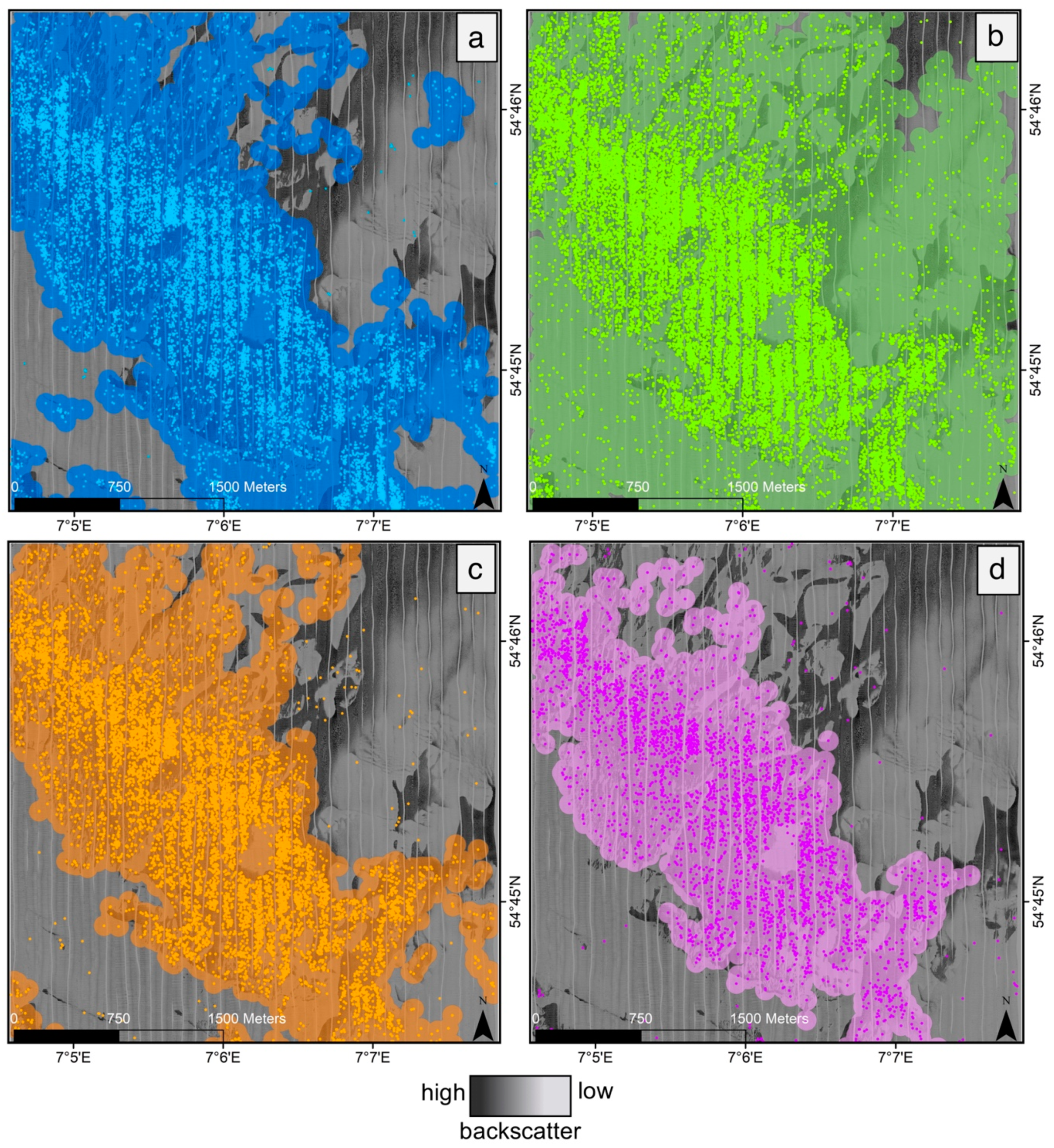
The demarcation of the geogenic reef type based on the method of [23] applied on manually tagged stones revealed four distinct areas in the size of 0.075 km2 up to 8.052 km2 with a total size of 8.675 km2 (Figure 7a). The major part of the reef was aligned from the north-western to the south-eastern part of the study site.
The largest reef areas identified with the automated method were found at a threshold value of 6 at any of the different numbers of grey values (Table 5). Here, up to 99% of the reef area obtained from the manual method was shared by the automatically identified reef area. The lowest overlap was found for the SSS mosaic displayed with 32 grey values and a detector threshold of 20 (53%). The size of the area that is not shared with the manually derived reef area (i.e., lies outside of it) is also shown in Table 5. The largest area protrusion was found for a threshold value of 6 for any number of grey values (up to 3.71 km2). The lowest was observed for a threshold value of 20 at any number of grey values with less than 0.04 km2.
3.4. Selection of a Proper Threshold and Grey Value Combination
The results of the decision support (see Equation (1), Section 2.3) to identify the most valuable detector threshold and grey value combination is shown in Table 6 with a priority on the correctly predicted reef area (), and in Table 7 with a priority on the correctly identified number of stones (). The best results were continuously found for a threshold value of 10 with 128 grey values irrespective of the chosen distance between the manually and automatically classified stones.
3.5. Accuracy on Different Seafloor Types
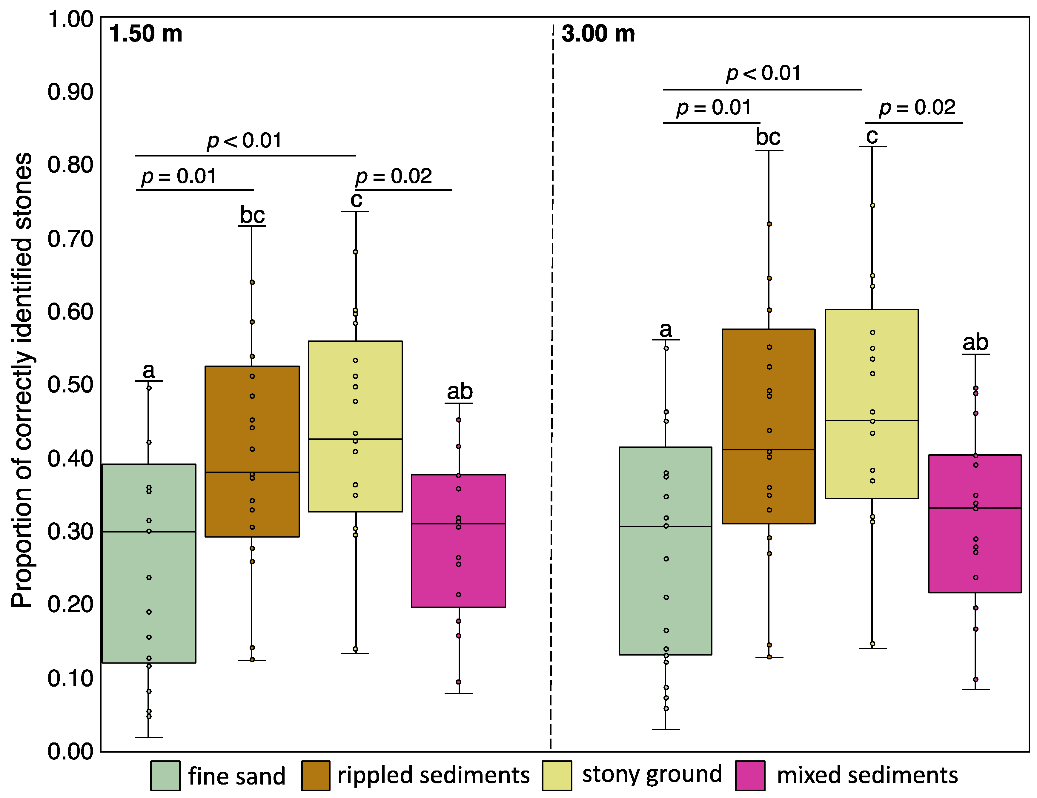
The study area was divided into 20,375 grid cells with 6996 cells corresponding to fine sand, 1951 cells to rippled sediments, 2549 cells to stony grounds and 8879 cells to mixed sediments (Figure 8). Statistically significant differences were found between the proportion of correctly identified stones and the different sediment types (one-way ANOVA: p < 0.001, F = 6.18, n per sediment type = 25). The proportion of correctly identified stones was higher on rippled sediments and stony grounds when compared to fine sand, and on stony grounds when compared to mixed sediments (Tukey–Kramer post-hoc test: p < 0.05; Figure 9). The proportion of correctly identified stones was lower for the 1.50 m buffer size. However, it was statistically not significant (p > 0.05, two-sample t-test).
4. Discussion
The detection of individual stones on SSS mosaics using Haar-like feature detectors was shown to be a promising approach for the purpose of stone identification and reef demarcation in benthic habitats. While other methods of detecting stones, e.g., the manual tagging or the application of pSES, are either time-consuming or lack the spatial distribution as they have a small footprint [13], this automatic method extracts the coordinates of potential stones on an SSS mosaic within a short amount of time. However, it requires the preparation of an adequate dataset for the training of the detector.
However, the detection of stones on an SSS mosaic using Haar-like feature detectors requires an optimal tuning of the training and detection procedure. Challenges appear on four levels: (1) the training of the detector, (2) the settings during the detection, (3) the quality and resolution of the SSS mosaic, and (4) the general performance of the detector with respect to different sediment types.
(1) The training of a Haar-like feature detector requires an a priori specification of settings related to the size of the detector (i.e., size of the rectangle, in pixels). The detection of relatively small objects (approx. smaller than 8x8 pixels on an SSS mosaic with a pixel resolution of 25 cm) requires a detector which was trained at least in the same size or smaller than the particular object. This, however, increases false-positive detections, as, e.g., the scattered noise of the mosaic might be interpreted as individual objects. Concomitantly, a detector, which was trained for larger objects, will miss smaller objects [28]. A large detector might further become sensitive for extensive transitions between sediments showing a prominent change of the acoustic backscatter (e.g., fine sand to coarse sand, cf., Figure 1d). Hence, selection of the appropriate size for the detector implies a trade-off between the general detection rate of objects and a small amount of false-positive detections. Most importantly, a large training dataset consisting of both positive and negative images is required for optimal training and an accurate detector [28]. In particular, for special applications such as the detection of stones such a training dataset cannot as yet be obtained elsewhere like training sets for objects such as faces, cars, trees and the like (e.g., Open Images Dataset [29] and MS-COCO [30]). So far, it needs to be created manually, which is a time-consuming procedure.
(2) The settings during the detection process also imply the specification of minimum and maximum sizes of the detector. This specification calls for the same trade-off, which was mentioned above. Additionally, the size of the detector must not be smaller than the size of the trained detector. Further, a merging threshold can be set that defines the degree to which multiple detections within a certain area will be combined into one single detection. Even though a higher threshold value allows the reduction of the number of false-positive detections, the number of missed objects might also increase (e.g., in an area of closely accumulated objects) as shown in this study. The results of this study might also be influenced by the different sources of the data used for the training (i.e., unprocessed data) and the data on which the detector was applied on (i.e., processed mosaic). However, we assume that this influence is of minor importance, as the samples used for the training of Haar-like features are generally manipulated in terms of, e.g., brightness or contrast, to achieve a higher number of training samples. The different sources further prevent the detector from becoming too specific, especially when the number of available training samples is low.
(3) Apart from the resolution of the SSS mosaic, the quality of the SSS data and the post-processing procedure also influence the performance of the detector (e.g., [31,32]). For example, nadir-stripes or strong noise caused by, e.g., bad weather conditions, might increase false-positive detections. A subsequent smoothing or hiding of such artefacts during the post-processing of the mosaic can only be achieved at the cost of a diminished mosaic resolution or a minimized spatial coverage. Haar-like feature detectors are furthermore known to be very sensitive for sonar illumination methods and the amount of lighting or soil type variation [33]. This was also shown in the results of this study, in which the number of detections follows an optimum curve with regard to the number of grey values. Most detections were observed for a mosaic displayed in 64 grey values. This might be caused by an optimum ratio of bright to black grey values, which increases the number of detections. However, future studies should investigate the effect of a detector trained on images with a broad range of number of grey values. So far, this detector only works on north–south oriented mosaics. It would hence be necessary to rotate the mosaics to the north–south orientation prior the procedure. The obtained results must then be rotated back to fit on the original mosaic.
(4) The seafloor in the form of the backscatter mosaic has a strong influence on the performance of the detector. Unexpectedly, the proportion of correctly identified stones was higher in areas with ripples and accumulations of stones than in areas with a homogeneous backscatter (e.g., stones lying on fine sand). This, however, seems to be the result of the training dataset that to a large degree consisted of images of stones from stony grounds (approx. 80%). Such a phenomenon was also observed in [15], where a sand ripple bottom type caused a large number of false-positive detections as a consequence of an unbalanced training dataset. A larger number of images of stones from homogeneous backscatter regions is therefore expected to improve the accuracy of detections for this type of backscatter. Furthermore, small depressions such as pock marks resemble the backscatter pattern of stones and tend to be misinterpreted in the identification process. Specially trained detectors can be used for subsequent clean-up procedures to identify pock marks and reject them from the stone data base. The detection of holes could be avoided by the training of a site-specific detector, i.e., one for the port- and one for the starboard channel. Such a detector constellation could be applied to a mosaic that only consists of track lines with the same heading and channel. However, visual mosaic inspection and underwater video footage suggest that both pock marks and deep holes do not occur within this study area.
So far, manually tagged stones are the only reliable criteria to assess the accuracy of a detector used for the detection of stones. This method, however, is also prone to mistakes. Especially in areas showing a dense accumulation of stones, the number of stones can be easily underestimated, as they might be difficult to demarcate from their surrounding neighbors. It therefore seems to be very unlikely that the detection of each single stone in such areas would be possible with either manual or automatic methods. Underestimation also happens for small stones or those buried to a certain degree under mobile sands. These stones do not show a recognizable shadow as a consequence of either too low mosaic pixel resolution or because they are located too close to the nadir. Michaelis et al. [9] have shown that the number of cobbles (6.3–20 cm) is approx. 25-fold larger than the number of boulders (20–63 cm) in the SOR. This underestimation lowers the calculated detection accuracy of a detector and may increase the number of detections mistakenly classified as false-negative detections. In general, even though false-negative detections might occur, they are not as critical for the purpose of reef demarcation as for the identification of, e.g., mine-like objects [34]. Furthermore, meaningful receiver operating characteristic curves (ROCs), which are commonly used to visualize the accuracy of a detector, cannot be provided under these circumstances, as they are based on the clear differentiation between positive and negative samples. This is, however, not possible with regard to stony areas on SSS mosaics. Uncertain cases can only be solved, if at all, with an area-wide ground truthing campaign (e.g., using underwater videos), which itself would be very time- and cost-intensive. Nevertheless, the need for rapid classification techniques is mandatory to meet the demands of, e.g., the European Union’s Habitats Directive (92/43/EEC), and to improve the quality of seabed sediment maps with regard to the patchy distribution of rocks (e.g., [35]).
The next step will be to improve the stone detector with an increase in the number of training images and to apply it on the whole SSS dataset available from the SOR. It would be further interesting to investigate the performance of the detector with regard to different SSS systems.
5. Conclusions
The identification and positioning of individual stones on SSS mosaics is a challenging and time-consuming but crucial process when it comes to the precise demarcation of reefs or the estimation and monitoring of the number of available anchor points for sessile organisms. In this study, we were able to demonstrate that the training and application of Haar-like feature detectors is a promising method to obtain the positions of individual stones on large SSS mosaics within a short detection time. An adequate demarcation of a reef is possible based on this data and can hence be used for monitoring purposes. Nevertheless, future studies should ensure the use of a well-balanced set of training images with respect to stones embedded in different sediment types to increase the general accuracy of the detector as well as to apply the detector on SSS mosaics from different study sites. We recommend building an open-source database providing labelled SSS training images from different SSS models to increase the amount of data available for the purpose of machine learning techniques. It should be further considered to tag and extract images of stones from SSS during long-lasting field surveys.
Author Contributions
Conceptualization, R.M., H.C.H. and S.P.; Formal analysis, R.M.; Funding acquisition, R.M., H.C.H. and S.P.; Investigation, R.M., H.C.H. and S.P.; Methodology, R.M.; Supervision, H.C.H. and K.H.W.; Visualization, R.M. and S.P.; Writing—review and editing, H.C.H., S.P. and K.H.W.
Funding
Data of this work were generated within the project AMIN I–III, a research and development cooperation between the Alfred Wegener Institute Helmholtz Centre for Polar and Marine Research and the Federal Maritime and Hydrographic Agency in Hamburg (BSH). It is part of the project SedAWZ coordinated by the BSH and financed by the Federal Agency for Nature Conservation (BfN).
Acknowledgments
We wish to thank the crew of the research vessel Heincke for their support during our research surveys and two unknown reviewers for their assistance to improve the manuscript.
Conflicts of Interest
The authors declare no conflict of interest.
References
- Sheehan, E.V.; Bridger, D.; Attrill, M.J. The ecosystem service value of living versus dead biogenic reef. Estuar. Coast. Shelf Sci. 2015, 154, 248–254. [Google Scholar] [CrossRef]
- Taylor, R.B. Density, biomass and productivity of animals in four subtidal rocky reef habitats: The importance of small mobile invertebrates. Mar. Ecol. Prog. Ser. 1998, 172, 37–51. [Google Scholar] [CrossRef]
- Airoldi, L. The effects of sedimentation on rocky coast assemblages. Oceanogr. Mar. Biol. Annu. Rev. 2003, 41, 161–263. [Google Scholar]
- Butchart, S.H.; Walpole, M.; Collen, B.; Van Strien, A.; Scharlemann, J.P.; Almond, R.E.; Carpenter, K.E. Global biodiversity: Indicators of recent declines. Science 2010, 328, 1164–1168. [Google Scholar] [CrossRef] [PubMed]
- Wiltshire, K.H. Urbanization of coastal and shelf seas. In Proceedings of the Conference Proceedings COME Decommissioning of Offshore Geotechnical COME-Decommissioning 2017, Hamburg, Germany, 28–29 March 2017. [Google Scholar]
- Bond, T.; Langlois, T.J.; Partridge, J.C.; Birt, M.J.; Malseed, B.E.; Smith, L.; McLean, D.L. Diel shifts and habitat associations of fish assemblages on a subsea pipeline. Fish. Res. 2018, 206, 220–234. [Google Scholar] [CrossRef]
- Meyer, K.S.; Brooke, S.D.; Sweetman, A.K.; Wolf, M.; Young, C.M. Invertebrate communities on historical shipwrecks in the western Atlantic: Relation to islands. Mar. Ecol. Prog. Ser. 2017, 566, 17–29. [Google Scholar] [CrossRef]
- Michaelis, R.; Hass, H.C.; Mielck, F.; Papenmeier, S.; Sander, L.; Gutow, L.; Wiltshire, K.H. Epibenthic assemblages of hard-substrate habitats in the German Bight (South-Eastern North Sea) described using drift videos. Cont. Shelf Res. 2019, 175, 30–41. [Google Scholar] [CrossRef]
- Michaelis, R.; Hass, H.C.; Mielck, F.; Papenmeier, S.; Sander, L.; Ebbe, B.; Gutow, L.; Wiltshire, K.H. Hard-substrate habitats in the German Bight (South-Eastern North Sea) observed using drift videos. J. Sea Res. 2019, 144, 78–84. [Google Scholar] [CrossRef]
- Schwarzer, K.; Bohling, B.; Heinrich, C. Submarine hard-bottom substrates in the western Baltic Sea–human impact versus natural development. J. Coast. Res. 2014, 70, 145–150. [Google Scholar] [CrossRef]
- Beldowski, J.; Klusek, Z.; Szubska, M.; Turja, R.; Bulczak, A.I.; Rak, D.; Jakacki, J. Chemical munitions search & assessment—An evaluation of the dumped munitions problem in the Baltic Sea. Deep Sea Res. Part II Top. Stud. Oceanogr. 2016, 128, 85–95. [Google Scholar] [CrossRef]
- Li, D.; Tang, C.; Xia, C.; Zhang, H. Acoustic mapping and classification of benthic habitat using unsupervised learning in artificial reef water. Estuar. Coast. Shelf Sci. 2017, 185, 11–21. [Google Scholar] [CrossRef] [Green Version]
- Papenmeier, S.; Hass, H.C. Detection of stones in marine habitats combining simultaneous hydroacoustic surveys. Geosciences 2018, 8, 279. [Google Scholar] [CrossRef]
- Reed, S.; Petillot, Y.; Bell, J. An automatic approach to the detection and extraction of mine features in sidescan sonar. IEEE J. Ocean. Eng. 2003, 28, 90–105. [Google Scholar] [CrossRef] [Green Version]
- Barngrover, C.; Kastner, R.; Belongie, S. Semisynthetic versus real-world sonar training data for the classification of mine-like objects. IEEE J. Ocean. Eng. 2015, 40, 48–56. [Google Scholar] [CrossRef]
- Lucieer, V.L. The application of automated segmentation methods and fragmentation statistics to characterise rocky reef habitat. J. Spat. Sci. 2007, 52, 81–91. [Google Scholar] [CrossRef]
- Sawas, J.; Petillot, Y. Cascade of boosted classifiers for automatic target recognition in synthetic aperture sonar imagery. Proc. Mtgs. Acoust. 2012, 17, 070074. [Google Scholar] [CrossRef]
- Atallah, L.; Smith, P.P.; Bates, C.R. Wavelet analysis of bathymetric sidescan sonar data for the classification of seafloor sediments in Hopvågen Bay-Norway. Mar. Geophys. Res. 2002, 23, 431–442. [Google Scholar] [CrossRef]
- Berthold, T.; Leichter, A.; Rosenhahn, B.; Berkhahn, V.; Valerius, J. Seabed sediment classification of side-scan sonar data using convolutional neural networks. In Proceedings of the IEEE Symposium Series on Computational Intelligence (SSCI), Honolulu, HI, USA, 27 November–1 December 2017; pp. 1–8. [Google Scholar] [CrossRef]
- Feldens, P.; Darr, A.; Feldens, A.; Tauber, F. Detection of boulders in side scan sonar mosaics by a neural network. Geosciences 2019, 9, 159. [Google Scholar] [CrossRef]
- Stewart, W.K.; Jiang, M.; Marra, M. A neural network approach to classification of sidescan sonar imagery from a midocean ridge area. IEEE J. Ocean. Eng. 1994, 19, 214–224. [Google Scholar] [CrossRef]
- Wen, X.; Shao, L.; Xue, Y.; Fang, W. A rapid learning algorithm for vehicle classification. Inf. Sci. 2015, 295, 395–406. [Google Scholar] [CrossRef]
- BfN 2018. BfN-Kartieranleitung für „Riffe“ in der Deutschen Ausschließlichen Wirtschaftszone (AWZ). Available online: https://www.bfn.de/fileadmin/BfN/meeresundkuestenschutz/Dokumente/BfN-Kartieranleitungen/BfN-Kartieranleitung-Riffe-in-der-deutschen-AWZ.pdf (accessed on 28 March 2019).
- Diesing, M.; Schwarzer, K. Identification of submarine hard-bottom substrates in the German North Sea and Baltic Sea EEZ with high-resolution acoustic seafloor imaging. In Progress in Marine Conservation in Europe; Springer: Berlin/Heidelberg, Germany, 2006; pp. 111–125. [Google Scholar] [CrossRef]
- Papenmeier, S.; Hass, H.C.; Propp, C.; Thiesen, M.; Zeiler, M. Verteilung der Sedimenttypen auf dem Meeresboden in der deutschen AWZ (1:10.000) 2018. Available online: http://www.geoseaportal.de (accessed on 6 May 2019).
- BSH. 2018. Available online: http://www.geoseaportal.de/ (accessed on 8 May 2018).
- Viola, P.; Jones, M. Rapid object detection using a boosted cascade of simple features. In Proceedings of the 2001 IEEE Computer Society Conference on Computer Vision and Pattern Recognition. CVPR 2001, Kauai, HI, USA, 8–14 December 2001. [Google Scholar] [CrossRef]
- Zhu, B.; Wang, X.; Chu, Z.; Yang, Y.; Shi, J. Active learning for recognition of shipwreck target in side-scan sonar image. Remote Sens. 2019, 11, 243. [Google Scholar] [CrossRef]
- Kuznetsova, A.; Rom, H.; Alldrin, N.; Uijlings, J.; Krasin, I.; Pont-Tuset, J.; Ferrari, V. The open images dataset v4: Unified image classification, object detection, and visual relationship detection at scale. arXiv 2018, arXiv:1811.00982. [Google Scholar]
- Lin, T.Y.; Maire, M.; Belongie, S.; Hays, J.; Perona, P.; Ramanan, D.; Zitnick, C.L. Microsoft coco: Common objects in context. In European Conference on Computer Vision 2014; Springer: Cham, Switzerland, 2014; pp. 740–755. [Google Scholar] [CrossRef]
- Lucieer, V.L. Object-oriented classification of sidescan sonar data for mapping benthic marine habitats. Int. J. Remote Sens. 2008, 29, 905–921. [Google Scholar] [CrossRef]
- Wang, X.; Zhao, J.; Zhu, B.; Jiang, T.; Qin, T. A side scan sonar image target detection algorithm based on a neutrosophic set and diffusion maps. Remote Sens. 2018, 10, 295. [Google Scholar] [CrossRef]
- Dzieciuch, I.; Gebhardt, D.; Barngrover, C.; Parikh, K. Non-linear convolutional neural network for automatic detection of mine-like objects in sonar imagery. In International Conference on Applications in Nonlinear Dynamics; Springer: Cham, Switzerland, 2016; pp. 309–314. [Google Scholar]
- Olmos, A.; Trucco, E. Detecting man-made objects in unconstrained subsea videos. In Proceedings of the OCEANS’02 MTS/IEEE, Biloxi, MI, USA, 29–31 October 2002; pp. 1–10. [Google Scholar] [CrossRef]
- Wilson, R.J.; Speirs, D.C.; Sabatino, A.; Heath, M.R. A synthetic map of the north-west European Shelf sedimentary environment for applications in marine science. Earth Syst. Sci. Data 2018, 10, 109–130. [Google Scholar] [CrossRef] [Green Version]
Figure 1.
Map of the position of the study area located within the German Bight in the south-eastern North Sea (a and b; side-scan sonar (SSS) mosaic from [13]). The SSS mosaic of the study area is shown in c. White vertical stripes in the SSS mosaic show the area of the clipped nadir. A close-up view of a part of the SSS mosaic is given in d. Bathymetric data were provided by the German Federal Maritime and Hydrographic Agency [26].

Figure 2.
Schematic workflow of the multiplication and final numbers of positive and negative training samples. Dark colors of the SSS mosaic represent high backscatter and bright colors represent low backscatter values.
Figure 2.
Schematic workflow of the multiplication and final numbers of positive and negative training samples. Dark colors of the SSS mosaic represent high backscatter and bright colors represent low backscatter values.

Figure 3.
Manually (blue) and automatically (orange) detected stones on an SSS mosaic (25-cm resolution) with buffer sizes of 3.00 m (a). The red area indicates the largest overlap between two spatially matching stones. The underlying SSS mosaic is shown in (b). White areas indicate the acoustic shadows of the stones.

Figure 4.
Schematic representation of the calculation of the factors used in Equation (1).

Figure 5.
Stones and detections on an SSS mosaic (25-cm resolution) with different methods: (a) manually tagged stones, and automatic detections on an SSS mosaic with 64 grey values and a detector threshold value of 6 (b), 12 (c) and 20 (d).
Figure 5.
Stones and detections on an SSS mosaic (25-cm resolution) with different methods: (a) manually tagged stones, and automatic detections on an SSS mosaic with 64 grey values and a detector threshold value of 6 (b), 12 (c) and 20 (d).

Figure 6.
Histogram of observed stone sizes in the area derived from manual measurements of a random sample (n = 1127).
Figure 6.
Histogram of observed stone sizes in the area derived from manual measurements of a random sample (n = 1127).

Figure 7.
Demarcated geogenic reef area and identified stones (points) on an SSS mosaic (25-cm resolution) with different methods: (a) manually, automatically on an SSS mosaic with 64 grey values and a detector threshold value of 6 (b), 12 (c) and 20 (d).
Figure 7.
Demarcated geogenic reef area and identified stones (points) on an SSS mosaic (25-cm resolution) with different methods: (a) manually, automatically on an SSS mosaic with 64 grey values and a detector threshold value of 6 (b), 12 (c) and 20 (d).

Figure 8.
Locations of the different sediment types within the study area based on 25 × 25 m grid cells (a). Close-up views of the sediment types are given in b–e. Dark colors of the SSS mosaic represent high backscatter and bright colors represent low backscatter values.
Figure 8.
Locations of the different sediment types within the study area based on 25 × 25 m grid cells (a). Close-up views of the sediment types are given in b–e. Dark colors of the SSS mosaic represent high backscatter and bright colors represent low backscatter values.

Figure 9.
Boxplot and results of the Tukey–Kramer post-hoc test between the proportion of correctly identified stones (based on a buffer size of 1.50 and 3.00 m between the automatically and manually derived stones) and the sediment types fine sand, rippled sediments, stony ground and mixed sediments. Different letters within a buffer-size class indicate statistically significant differences at a significant level of p < 0.05.


Table 1.
Number of detections on the SSS mosaic under different frame conditions. Color scale indicates high values in green and low values in red. The average Euclidian distance [m] to the nearest neighbor is given in parentheses.
Table 1.
Number of detections on the SSS mosaic under different frame conditions. Color scale indicates high values in green and low values in red. The average Euclidian distance [m] to the nearest neighbor is given in parentheses.
| Grey Values | ||||||
|---|---|---|---|---|---|---|
| 32 | 64 | 128 | 192 | 256 | ||
| Threshold | 6 | 12,062 (12.9) | 21,118 (8.9) | 13,389 (11.4) | 13,133 (11.5) | 13,105 (11.5) |
| 8 | 8193 (14.5) | 15,410 (9.7) | 9375 (13.0) | 9242 (13.1) | 9240 (13.2) | |
| 10 | 5886 (16.1) | 11,619 (10.6) | 7100 (14.5) | 6918 (14.6) | 6902 (14.6) | |
| 12 | 4374 (18.1) | 9069 (11.7) | 5444 (16.1) | 5291 (16.4) | 5293 (16.3) | |
| 20 | 1544 (26.2) | 3674 (17.5) | 1801 (28.4) | 1745 (28.2) | 1749 (28.8) | |
Table 2.
Number of matching stones between the automatic and manual detection methods under different frame conditions at a buffer size of 1.50 m. Color scale indicates high values in green and low values in red. The proportion to the total number of automatically detected stones are in parentheses.
| Grey Values | ||||||
|---|---|---|---|---|---|---|
| 32 | 64 | 128 | 192 | 256 | ||
| Threshold | 6 | 4726 (0.39) | 7389 (0.35) | 6607 (0.49) | 6495 (0.49) | 6489 (0.50) |
| 8 | 4002 (0.49) | 6660 (0.43) | 5576 (0.59) | 5490 (0.59) | 5495 (0.59) | |
| 10 | 3379 (0.57) | 5826 (0.50) | 4732 (0.67) | 4628 (0.67) | 4612 (0.67) | |
| 12 | 2836 (0.65) | 5100 (0.56) | 3940 (0.72) | 3812 (0.72) | 3817 (0.72) | |
| 20 | 1274 (0.83) | 2732 (0.74) | 1518 (0.84) | 1473 (0.84) | 1473 (0.84) | |
Table 3.
Number of matching stones between the automatic and manual detection methods under different frame conditions at a buffer size of 3.00 m. Color scale indicates high values in green and low values in red. The proportion to the total number of automatically detected stones are in parentheses.
| Grey Values | ||||||
|---|---|---|---|---|---|---|
| 32 | 64 | 128 | 192 | 256 | ||
| Threshold | 6 | 5152 (0.43) | 7919 (0.37) | 7026 (0.52) | 6902 (0.53) | 6900 (0.53) |
| 8 | 4331 (0.53) | 7109 (0.46) | 5908 (0.63) | 5807 (0.63) | 5828 (0.63) | |
| 10 | 3650 (0.62) | 6201 (0.53) | 4990 (0.70) | 4873 (0.70) | 4859 (0.70) | |
| 12 | 3042 (0.70) | 5389 (0.59) | 4132 (0.76) | 3994 (0.75) | 3999 (0.76) | |
| 20 | 1352 (0.88) | 2872 (0.78) | 1576 (0.88) | 1530 (0.88) | 1534 (0.88) | |
Table 4.
Proportion of matching stones between the automatic detection method and the total amount of the manual detection method (n = 12,852) under different frame conditions using the 1.50 m buffer size (3.00 m in parentheses). Color scale indicates high values in green and low values in red.
Table 4.
Proportion of matching stones between the automatic detection method and the total amount of the manual detection method (n = 12,852) under different frame conditions using the 1.50 m buffer size (3.00 m in parentheses). Color scale indicates high values in green and low values in red.
| Grey Values | ||||||
|---|---|---|---|---|---|---|
| 32 | 64 | 128 | 192 | 256 | ||
| Threshold | 6 | 0.37 (0.40) | 0.57 (0.62) | 0.51 (0.55) | 0.51 (0.54) | 0.50 (0.54) |
| 8 | 0.31 (0.34) | 0.52 (0.55) | 0.43 (0.46) | 0.43 (0.45) | 0.43 (0.45) | |
| 10 | 0.26 (0.28) | 0.45 (0.48) | 0.37 (0.39) | 0.36 (0.38) | 0.36 (0.38) | |
| 12 | 0.22 (0.24) | 0.40 (0.42) | 0.31 (0.32) | 0.30 (0.31) | 0.30 (0.31) | |
| 20 | 0.10 (0.11) | 0.21 (0.22) | 0.12 (0.12) | 0.11 (0.12) | 0.11 (0.12) | |
Table 5.
Proportion of the manual reef area shared with the model-predicted one after the method proposed by [23] under different frame conditions. Color scale indicates high values in green and low values in red. The predicted reef area [km2] not shared with the manually derived one (= 8.675 km2) is given in parentheses.
| Grey Values | ||||||
|---|---|---|---|---|---|---|
| 32 | 64 | 128 | 192 | 256 | ||
| Threshold | 6 | 0.99 (3.405) | 0.99 (3.710) | 0.99 (3.385) | 0.99 (3.370) | 0.99 (3.516) |
| 8 | 0.97 (2.395) | 0.92 (1.440) | 0.98 (2.104) | 0.97 (2.170) | 0.98 (2.262) | |
| 10 | 0.91 (1.345) | 0.89 (0.721) | 0.95 (1.021) | 0.94 (1.034) | 0.94 (1.135) | |
| 12 | 0.79 (0.605) | 0.84 (7.614) | 0.88 (0.605) | 0.90 (0.558) | 0.91 (0.564) | |
| 20 | 0.53 (0.005) | 0.63 (0.044) | 0.64 (0.019) | 0.63 (0.015) | 0.63 (0.000) | |
Table 6.
Decision support for the identification of the most valuable detector threshold and grey value combination with a priority on the correctly predicted reef area. Values represent the results for a buffer size of 1.50 m (3.00 m in parentheses) between the manually and automatically classified stones. Values close to 0.01 are more similar to the manual method. Color scale indicates good values in green and bad values in red.
| Grey Values | ||||||
|---|---|---|---|---|---|---|
| 32 | 64 | 128 | 192 | 256 | ||
| Threshold | 6 | 1.67 (1.44) | 1.14 (1.03) | 1.00 (0.88) | 1.01 (0.89) | 1.01 (0.89) |
| 8 | 1.66 (1.42) | 1.13 (1.01) | 0.95 (0.82) | 0.97 (0.84) | 0.96 (0.83) | |
| 10 | 1.66 (1.38) | 1.15 1.02) | 0.93 (0.79) | 0.95 (0.81) | 0.95 (0.81) | |
| 12 | 1.70 (1.40) | 1.17 (1.04) | 0.95 (0.80) | 0.99 (0.83) | 0.98 (0.83) | |
| 20 | 2.08 (1.50) | 1.43 (1.20) | 1.54 (1.23) | 1.57 (1.25) | 1.59 (1.25) | |
Table 7.
Decision support for the identification of the most valuable detector threshold and grey value combination with a priority on the amount of correctly identified stones. Values represent the results for a buffer size of 1.50 m (3.00 m in parentheses) between the manually and automatically classified stones. Values close to 0.10 are more similar to the manual method. Color scale indicates good values in green and bad values in red.
| Grey Values | ||||||
|---|---|---|---|---|---|---|
| 32 | 64 | 128 | 192 | 256 | ||
| Threshold | 6 | 2.85 (2.15) | 1.39 (1.14) | 1.08 (0.86) | 1.11 (0.89) | 1.11 (0.88) |
| 8 | 2.84 (2.10) | 1.39 (1.14) | 1.00 (0.78) | 1.04 (0.81) | 1.03 (0.79) | |
| 10 | 2.83 (2.00) | 1.43 (1.16) | 0.98 (0.75) | 1.02 (0.78) | 1.02 (0.78) | |
| 12 | 2.87 (1.99) | 1.48 (1.20) | 1.04 (0.79) | 1.10 (0.83) | 1.08 (0.82) | |
| 20 | 3.66 (1.96) | 1.93 (1.43) | 2.23 (1.50) | 2.31 (1.54) | 2.36 (1.53) | |
© 2019 by the authors. Licensee MDPI, Basel, Switzerland. This article is an open access article distributed under the terms and conditions of the Creative Commons Attribution (CC BY) license (http://creativecommons.org/licenses/by/4.0/).
Share and Cite
MDPI and ACS Style
Michaelis, R.; Hass, H.C.; Papenmeier, S.; Wiltshire, K.H. Automated Stone Detection on Side-Scan Sonar Mosaics Using Haar-Like Features. Geosciences 2019, 9, 216. https://doi.org/10.3390/geosciences9050216
AMA Style
Michaelis R, Hass HC, Papenmeier S, Wiltshire KH. Automated Stone Detection on Side-Scan Sonar Mosaics Using Haar-Like Features. Geosciences. 2019; 9(5):216. https://doi.org/10.3390/geosciences9050216
Chicago/Turabian StyleMichaelis, Rune, H. Christian Hass, Svenja Papenmeier, and Karen H. Wiltshire. 2019. "Automated Stone Detection on Side-Scan Sonar Mosaics Using Haar-Like Features" Geosciences 9, no. 5: 216. https://doi.org/10.3390/geosciences9050216
Note that from the first issue of 2016, this journal uses article numbers instead of page numbers. See further details here.