1. Introduction
Large parts of the deep ocean floor are covered with fine-grained sediments that contain high amounts of clay minerals [
1]. These so-called red clays represent about 50% of the sediments in the Pacific Ocean and occur in areas of low biological productivity and beneath the Carbonate Compensation Depth (CCD) [
2]. The sediment accumulation is low and favourable for the formation of manganese (Mn) nodules [
3]. The clays in these sediments originate mainly from weathering processes on the continents and from hydrothermal alteration of surficial oceanic crust, and they are transported into the ocean either as aerosols or in suspension [
4,
5,
6]. The suspended particulate matter (SPM) in the deep water overlying the seabed exhibits in low concentrations (<0.05 mg/L) and consists of a hardly settling fine fraction (size of 1–10 µm) and a faster settling larger fraction (up to 1 mm) [
7]. The latter is associated with the formation of aggregates of mainly biological origin, also called marine snow [
8].
Recent developments in technology for depths >4000 m have led to a new interest for Mn-nodule mining to satisfy the increasing needs for rare earth elements and metals such as cobalt, nickel and copper. However, a large-scale exploitation inherently raises questions about the impacts and effects on the marine ecosystem [
9]. Besides the direct removal of the sediment layer (nodule habitat), the associated formation of sediment plumes, with much higher SPM concentration (SPMC) than the natural concentration, will result in blanketing large areas around the mining site with multiple impacts on deep-sea ecosystems.
Since the 1970s, major explorative studies have been carried out, including the United States Deep Ocean Mining Environmental Study (DOMES) in the eastern Pacific Ocean (e.g., [
10,
11] and the DISCOL (DISturbance and re-COLonization Experiment) project in the SE Pacific Ocean and its follow-up project ATESEPP (Effects of Technical Interventions into the Ecosystem) (e.g., [
12,
13,
14,
15]). In more recent years, the well-known occurrence of Mn-nodules in the Clarion–Clipperton Fracture zone (CCZ) in the NE equatorial Pacific Ocean is subject to industrial exploration and associated scientific research [
16].
The present study was part of the first phase (2015–2017) of the “MiningImpact” project focusing on the Ecological Aspects of Deep-sea Mining, funded by the Joint Programming Initiative Healthy and Productive Seas and Oceans of the European science foundations. In the framework of this project, two expeditions with the German RV Sonne were carried out (SO239 and SO242), revisiting areas in the abyssal Pacific Ocean (SO239 to the CCZ) which had been subjected to disturbance experiments in the past three decades. The main objective of the second expedition (SO242) was to revisit the DISCOL area in the Peru Basin for high-detail mapping and biogeochemical and biological sampling in both disturbed (ploughed in 1989) and undisturbed areas. In this study, a small-scale seafloor disturbance experiment was carried out to investigate the dispersion of the generated sediment plumes by near-bottom currents.
A key element in understanding the footprint of sediment plumes produced by deep-sea mining is the settling behaviour of the particles within the plume and the erosion potential of redeposited particles. Currents in the deep ocean are typically slow (few cm/s) and are not able to erode seafloor sediments but are able to keep fine sediment particles in suspension [
7]. Laboratory experiments with sediments from the CCZ area have shown that depending on the SPMC and the turbulence, flocculation may occur, resulting in higher settling velocities and thus a faster deposition of the plume sediments [
17]. Several authors have pointed out that the occurrence of meso-scale eddies may result in resuspension of the freshly deposited particles from a plume, which could result in a long-term increase of the turbidity in a larger area around the mining site [
17,
18,
19,
20].
The objectives of this study are:
- (1)
Investigate the natural background SPMC and its increase due to mechanical mobilisation of seafloor sediments;
- (2)
Characterize the seafloor sediment (such as mud fraction and flocculation potential) and ambient tidal current dynamics of the deep-sea that lead to sediment dispersion and subsequent redeposition;
- (3)
Test to what extent the observed plume dispersion and dynamics by near-bed currents are reproduced by the ocean dynamics and sediment transport model presented in [
21].
Study Area
Located in the Peru Basin (southern Pacific Ocean), the area of interest is 900 km offshore Peru at 7.12° south of the equator (
Figure 1), lying in water of around 4150 m depth. The area is known as the DISCOL Experimental Area (DEA), where in 1989, a circular patch of about 2 nautical miles across was impacted with a plough–harrow to generate a mechanical disturbance. The topographically gently sloping DEA, with a lower Mn-nodule density than the surrounding and without rocky outcrops, was chosen to avoid failure of the plough [
9]. The area is part of a north–south trending graben-horst system with presence of seamounts [
22,
23]. The experimental site is in the Reference Area South (of the DEA) with presence of Mn-nodules (
Figure 1c), characterized with slopes up to 8° [
24].
The CCD in the Peru Basin at present varies between 4200 and 4350 m [
14]. As a result, surface sediment of areas deeper than 4200 m generally have a low carbonate content, as compared to sediment at shallower depths [
14]. In the past, vertical CCD fluctuations were a result of sequences of glacial and interglacial phases [
25]. The average Mn-nodule abundance is 9 kg/m
2 [
24], similar to what is found in the wider Peru Basin [
26,
27]. The natural sediment accumulation rate is estimated as 2 cm/ky [
3].
The water mass near the bottom in the DISCOL is characterized by salinity of about 35 PSU and temperature <2 °C, and currents with alternating regimes: weak (1–3 cm/s) and strong (~5 cm/s) episodes [
12,
13].
The DISCOL seafloor sediments are vertically divided into three zones based on their physico-chemical characteristics [
14,
28]: a dark brown semi-liquid top layer (5–15 cm thickness) contains Mn-nodules, a transition zone of light sediment colour with increasing shear strength (5–15 cm), and an underlying light grey consolidated layer.
2. Materials and Methods
2.1. Analysis of Seafloor Sediments
For analysis of surface sediment particle size distribution and mineralogy, multicores (MUC) from SO241 stations 34_MUC-6, 70_MUC-17 and 119_MUC-31, were sampled for the surface (0 to 5 cm) and deeper part (5–15 cm). All samples were first oven-dried at 40 °C and subsequently crushed by hand with mortar and pestle until they passed through a 500 µm sieve. From each sample, a representative subsample of 2.7 g was taken for the determination of the bulk mineralogical composition. As an internal standard, 0.3 g of Zincite (ZnO) was added. The powders were mixed and ground in a McCrone
® micronising mill in ethanol (Westmont, IL, USA). After drying, the samples were loaded in a sample holder by side-loading and measured by X-ray diffraction (using CuKα radiation). The subsequent quantification of bulk minerals was performed by using a combination of the Rietveld method [
29] and of the PONKCS method [
30]. The fraction <2 µm of a representative subsample of 5 g of each sample was separated. This size fraction is enriched in sedimentary clay minerals. The separation was performed after a thorough chemical treatment. Carbonate cements, organic matter and free Mn-, Fe-(hydr)oxides were removed using respectively acetic acid/Na-acetate buffer solution, 30% H
2O
2 solution and Na-dithionite in a Na-citrate-bicarbonate environment respectively. In this <2 µm fraction, all the minerals are exchanged to their Ca-form (e.g., the different cations that may occur in the interlayer of the Smectite mineral are all exchanged to Ca). Oriented preparation slides were made by sedimentation; the preparation yields highly oriented clay particles with their (001) lattice plains parallel oriented. The oriented slides were subsequently analysed by X-ray diffraction for measuring the refraction intensity of the 001 lattice plains of the clay minerals.
The organic carbon content in yet another subsample was determined by infrared analysis. This analysis is based on the combustion of the sample and the subsequent measurement of the IR-energy which is absorbed at a specific wavelength by a Leco CS 244 analyser.
The major element content of the samples was measured by ICP-MS analysis using a Perkin Elmer Sciex ELAN 6000. Yet another subsample was fused with lithium metaborate/tetraborate, diluted, and subsequently analysed with a Perkin Elmer Sciex ELAN 6000 ICP-MS. Additionally, the total amount of carbon and sulphur was determined using induction furnaces coupled to a Leco CS 244 analyser with infrared detector.
The grain-size volume distribution of the samples was measured with laser diffraction using a Malvern Mastersizer-S in water with ultrasound sonification. And more subsamples were measured (1) without preparation, only after shaking in water for 24 h and (2) after a thorough chemical treatment to remove the cementing agents and to break up aggregates.
2.2. BoBo and DOS Lander Deployment: Sensors
Near-bottom current dynamics and SPM transport were recorded with the Bottom Boundary (BoBo) lander of NIOZ and the Deep-sea Observation System (DOS) lander of GEOMAR (
Figure 2). The BoBo lander [
31] was equipped among other sensors with an RDI 1200 kHz ADCP (acoustic Doppler current profiler) mounted downward facing at 2 m above the seafloor (2 mab) in the centre of the lander frame and a Seabird 19 plus CTD (conductivity, temperature, depth) with Seapoint turbidity meter (hereafter called Seapoint) at 2.5 mab. The DOS lander, adapted from the multipurpose platform designed by [
32], was equipped with a similar Seabird CTD device positioned at 1 mab. The BoBo and DOS landers were deployed in free-fall mode.
For a period of 74 days (July–September 2015), the landers were co-deployed at 6 different stations (
Table 1 and
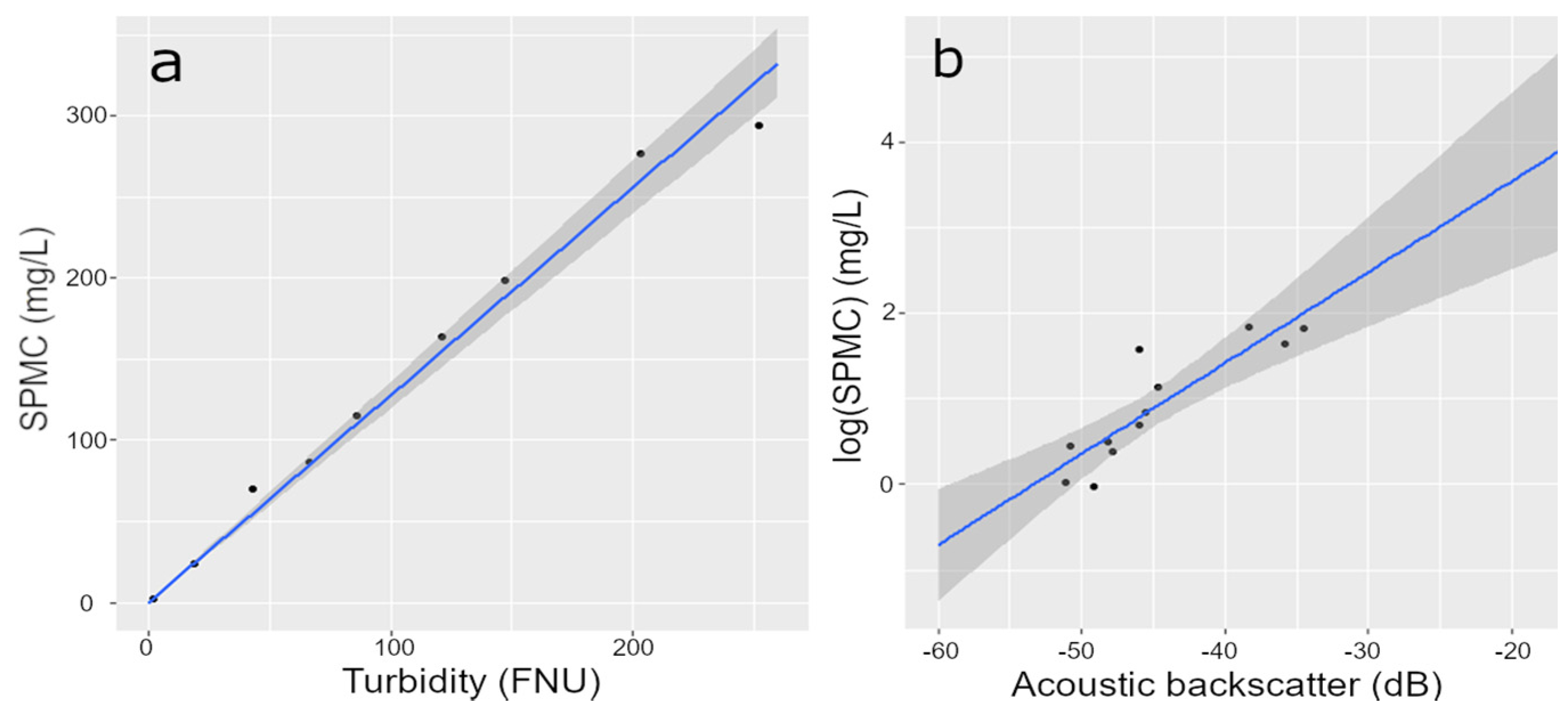
Figure 1b) within a perimeter of 17 km in water depths between 4150 and 4220 m. The CTDs were sampling in intervals of 300 sec with 5 measurements per sample. The Seapoints were set to measure over a range between 0 and 25 FNU (Formazine Nephelometric Unit). A unit conversion factor of 1.28 between turbidity (FNU) and SPMC (mg/L) was obtained through a series of suspensions of known SPMC prepared from in situ sediment and corresponding Seapoint FNU readings.
Figure 3a shows the linear regression with a determination coefficient (R
2) of 0.98. With their light source wavelength of 880 nm, Seapoints optimally work for fine-grained particles [
33,
34].
For the ambient hydrodynamics, the downward facing ADCP mounted on the BoBo lander collected 20 cm bin data in ensemble intervals of 300 sec with 50 pings per ensemble. Six percent of the near-seafloor data of the profiles (0.12 m) plus one bin is affected by side-lobe interference and were thus discarded resulting in a usable range of observations from 1.4 to 0.6 mab. The ADCP correlation magnitudes, which are the ultimate quality audit parameter for deep-sea environments [
35] were evaluated. The residual meridional and longitudinal velocities in the study area were obtained by removing the tidal components through a low-pass filter [
36]. Bottom shear velocities,
u*, were derived through the power law profile method [
37,
38], based on the following formula:
which analyses the linear relationship (with R
2 > 0.9) between the (5 min ensemble interval) current velocities,
u (m/s) and the corresponding logarithm of the bin heights above the seafloor (
z).
k is the von Karman constant (0.41) and
z0 (m) is the bed roughness length. The bottom shear stress τ (Pa) are then calculated from
u* and seawater density rho (1050 kg/m
3):
By knowing the water viscosity ʋ (m
2/s), the shear rates G (1/s) at a certain bin height (
z) can be calculated from the bottom shear velocities as follows [
39,
40,
41,
42]:
with
Additionally, the inversion of the raw ADCP acoustic backscatter to SPMC was realised after several corrections were applied [
43]: the ADCP noise level, the spherical beam spreading and the sound absorption by the water. Given the low SPMC, the sound attenuation due to SPM is negligible. Any observed increases in the inverted backscatter values are directly linked to increased SPMC. Noteworthy, is the capability of the ADCP to capture underwater noise.
2.3. Epi-Benthic Sledge (EBS): Seafloor Disturber and Sensor Platform
The EBS used in the experiment to generate a plume of suspended sediment is based on the sledge frame of [
44] and weights 880 kg (in air), is 3.6 m long, 2.4 m wide and 1.2 m high and intended for benthic epi- and macrofauna sampling (
Figure 2). An ultra-short baseline transponder provided the geo-referenced position of the sledge on the seafloor. Two EBS towing experiments were programmed (#37_EBS-1 and #45_EBS-2) in the reference area south. In the second plume experiment, the EBS (#45_EBS-2) was towed between 00:36 and 00:56 UTC of 5 August 2015, over 740 m, slightly uphill (2.8%, Δ depth is 21 m) at a quasi-constant speed of 0.62 m/s (
Table 1;
Figure 1c). It passed north of the BoBo lander in the closest distance of 68 m (
Figure 1c). The EBS was equipped with a 2 MHz Aanderaa Doppler-based recording current meter (RCM) and an external Seapoint measuring turbidity between 0 and 5 FNU. For a duration of 20 min, the EBS disturbed the seafloor leaving a 2.4 m wide and 740 m long erosion scour mark (total of 1776 m
2). During the period when the EBS was on the seafloor, the Seapoint was often saturated (90% of the time) but the 10% of available Seapoint data could be correlated with the RCM acoustic backscatter data to retrieve estimates of SPMC beyond the 5 FNU limit of this Seapoint. Both data sets included 10 s interval data and the linear regression was good (R
2 = 0.75;
Figure 3b).
2.4. Modelling of the Plume
The numerical model used, the MITgcm (General Circulation Model), is based on the incompressible Navier–Stokes equations [
45,
46]. The model domain includes the actual bathymetry covering an area of about 3 × 3 km with a horizontal resolution of 35 m and 200 vertical levels covering the entire water column, with thinner layers towards the seafloor and a 1 m resolution at the lowest levels. The horizontal resolution used in the model is coupled with the best available topography data obtained from the ship based EM122 12 kHz multibeam system and the resulting bathymetric grid of 35 × 35 m cell size [
24]. A new feature in the sediment transport equation was developed and coupled to the MITgcm to enable deep-sea sediment transport applications [
21]. The model can represent an unlimited number of user-defined sediment classes based on settling velocities. Here we used three sediment diameter size classes, 61.2, 10.4 and 1.65 µm, referred hereafter as 61, 10 and 2 µm classes based on the d90, d50 and d10 (laser diffraction volume distribution-based) percentiles of the untreated surface sediment of station #70-MUC-17 (
Table 2). The corresponding Stokes’ law settling velocities for 61, 10 and 2 µm classes are 1.67, 0.048 and 0.001 mm/s respectively (considering the deep-sea water viscosity and density) [
47]. measured similar settling velocities for mid-water plumes in the CCZ.
The sediment classes can be transported as SPM by advection and diffusion schemes available in MITgcm (direct spacetime method with flux limiting). The background horizontal water viscosity and sediment diffusivity were set to 10
−4 and 10
−5 m
2/s, respectively. In addition, the nonlocal parameterization scheme of [
48] was used to solve vertical mixing in the model. The SPM in the lowest cell may leave the cell due to deposition and accumulates on the seafloor. The deposited mass can be re-suspended when the bottom shear velocity at the lowest cell reaches the critical values for particle re-suspension. The model was run with a time step of 5 s for the period from 31 July to 4 August 2015 as spin up to reach steady state condition. The lateral boundary conditions are in situ hydrodynamic data from the BoBo lander (ADCP). The salinity and temperature were set to fixed values of 1.8 °C and 34.7 PSU as measured in situ by the CTDs. A release rate of 0.142 kg/s is obtained based on the model-observation validation for the SPMC at a height of 2–3 mab at the BoBo position. The release height of the sediment plume is expected to be in the 0–2 mab.
3. Results
3.1. Multi Corer (MUC) Data
The mineralogical analyses indicate that all the investigated samples (34_MUC-6, 70_MUC-17 and 119_MUC-31, for both 0–5 cm and 5–15 cm) have a similar composition (
Table A1). Layer silicates are the most prominent minerals (between 40 and 50%) in all the samples consisting of dominantly 2:1-layer silicates and much lower proportions of Kaolinite and traces of Chlorite. Other minerals are Quartz, K-feldspar, Plagioclase, Calcite, Dolomite, Siderite, Gypsum, Barite, Anatase and Apatite. Significant amounts of amorphous material occur in all the samples, ranging from 26.0% to 35.8%. Chemical analysis reveals that this is predominantly opal from the silica skeletons of radiolarians and diatoms (
Table A2). The relationship between carbonate dilution and higher associated opal content was found by [
28]. Percentage of carbonate is lowest (almost absent) in #119-MUC-31. The results of the clay mineralogical analysis show that the <2 µm fraction of all the samples consists of a mixture of Smectite, Illite, mixed-layer Illite/Smectite and Chlorite (
Table A3). Smectite is the dominant clay mineral species, ranging from 44.6% to 49.7%, followed by mixed-layer Illite/Smectite (17.2–24.5%) and Illite (14.9–21.2%). Mixed-layer Kaolinite/Smectite ranges from 5.8% to 10.5%. Kaolinite (3.6–4.9%) and Chlorite (1.5–2.9%) occur in the lowest proportions. The clay mineralogical compositions of the different samples do not show any trend or systematic differences (
Appendix A).
The organic carbon content of the different samples is relatively low and ranges between 0.7% and 1.08% (
Table A4). These results are in line with [
3]. No clear difference in chemical composition between the different samples was found (
Table A2).
In
Table 2 the parameters and percentiles of the particle size distribution of the analysed samples are shown.
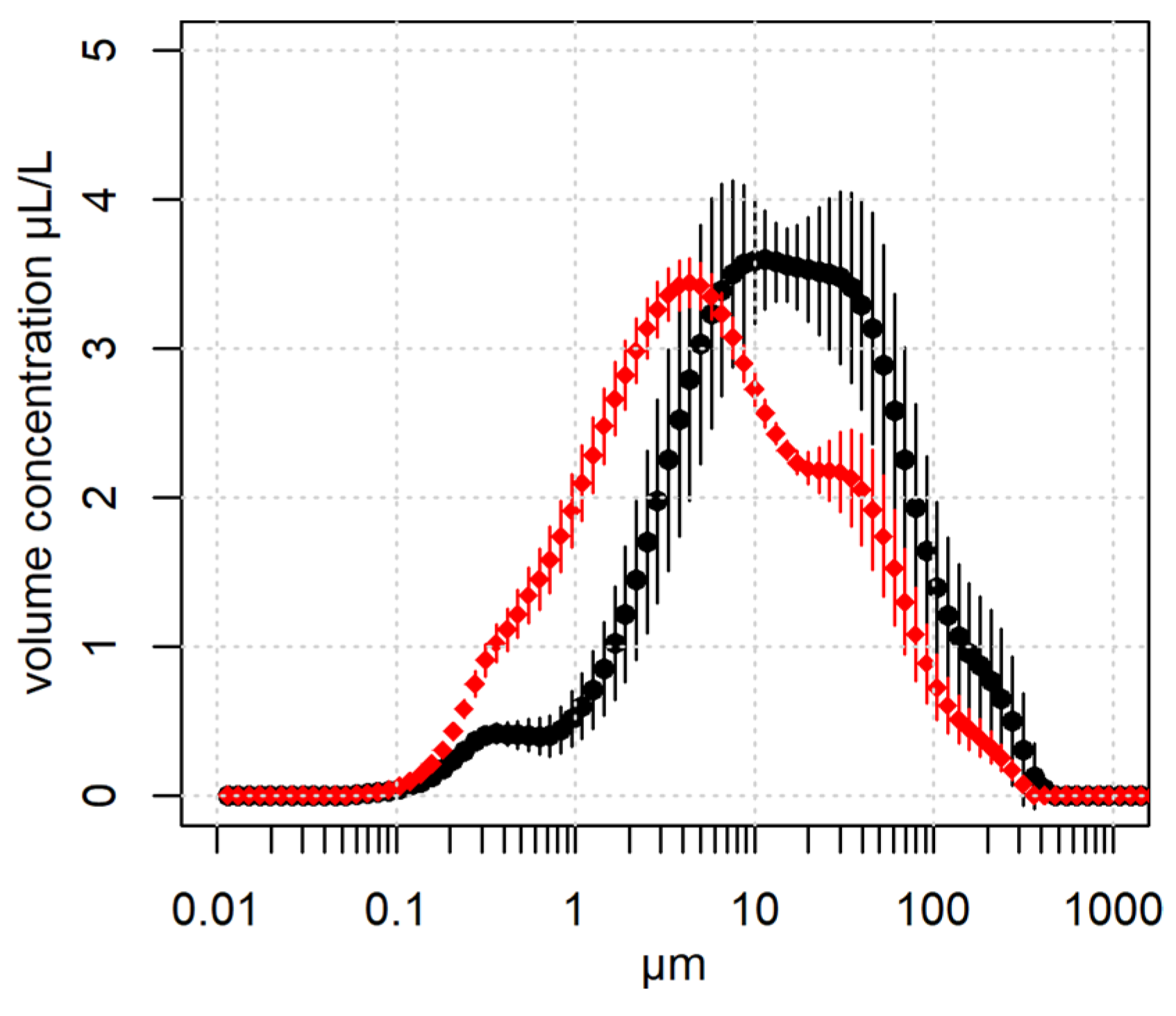
Figure 4 shows average particle size distributions, for the pre-treated and non-prepared samples. The main size modes from the non-prepared sample distributions are situated between 8 and 40 µm. Clay (<2 µm) percentages range between 7–12% for non-prepared samples, and between 20–30% for the pre-treated samples. Only about the half of the percentage of clay minerals seems to be in the <2 µm percentage. The presence of clay minerals in fractions >2 µm is possible. Alternatively, laser diffraction for grainsize measurements of clay minerals (which are platy) may result in slightly larger sizes. It seems that for our case, the <4 µm % comes closest to the clay mineral %.
3.2. BoBo and DOS Background Time-Series
The two CTDs mounted on the BOBO and DOS landers recorded a quasi-constant timeseries with water temperature of 1.8 °C and a salinity of 34.7 PSU. The measured tidal ranges as seen in the pressure data were between 0.5 and 1.6 m reflecting the fortnightly lunar cyclicity (neap and spring tides).
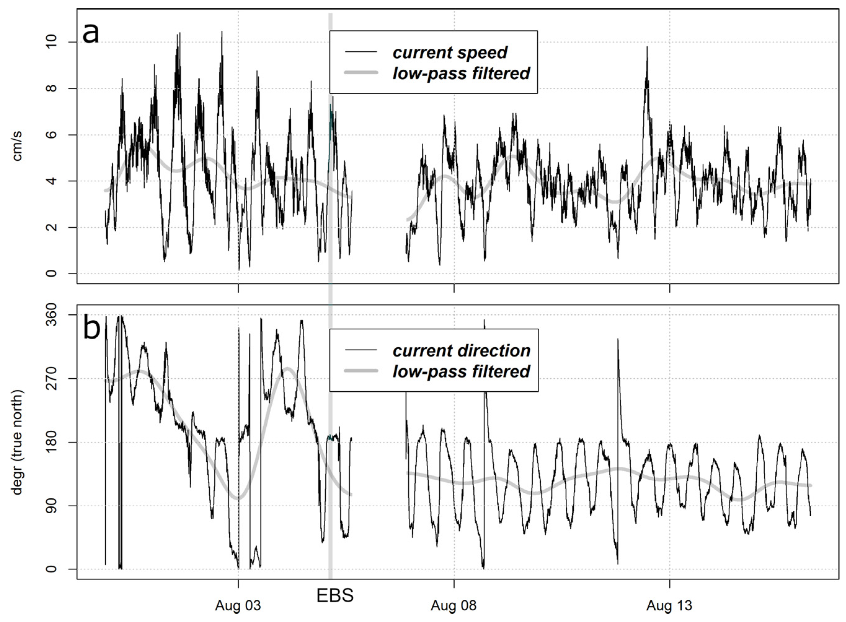
Figure 5a shows the ADCP time-series from two consecutive BoBo lander deployments (station #11_BoBo-lander-1 and station #57_BoBo lander 2,
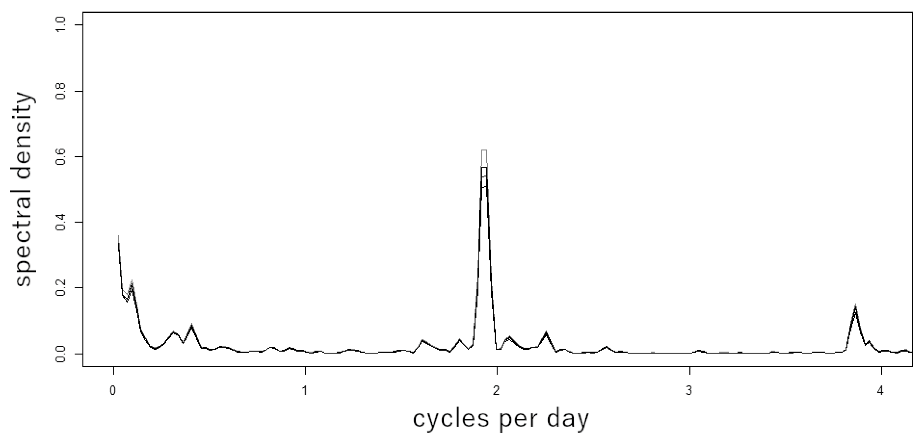
Appendix B). Current speeds measured at 1 mab with the downward looking 1200 kHz ADCP reach up to 10.5 cm/s, with an average of 4.0 cm/s. Turning tides obviously correspond to a decrease in current speed (slack tides). Spectral analysis indicates that the tidal currents were dominated by the semi-diurnal M2 constituent, followed by a quarter diurnal M4 constituent (
Figure A1). The average bottom shear velocity ranged from 0.07 to 0.8 cm/s, with an average of 0.3 cm/s, and the associated bottom shear stresses ranged between almost 0 and 0.06 Pa, with an average of 0.01 Pa. The shear rate is on average 0.25 1/s.
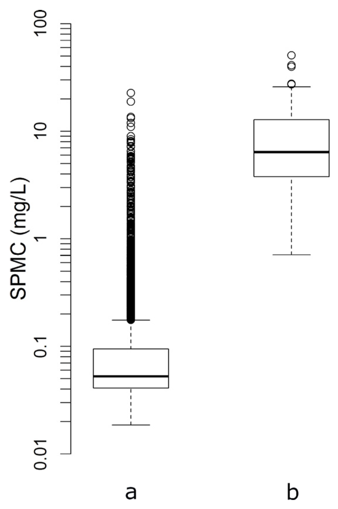
The Seapoint-SPMC data, for a total of 176 days (all BoBo and DOS deployments, see
Table 1), revealed low concentrations with a minimum of 0.02 mg/L and a median value of 0.05 mg/L (
Figure 6a). No tidal (M2 or M4) variability was found in the SPMC time-series, and there was no distinction in the background SPMC values between the Seapoint from the DOS (Seapoint at 1 mab) and the BoBo (Seapoint at 2.5 mab) landers. Outliers (up to 22.68 mg/L) are identified as momentary increases of SPMC caused by the sediment mobilisation by the BoBo and DOS lander upon landing on the seafloor.
3.3. BoBo Seafloor Disturbance Time Series of Sensors and Model
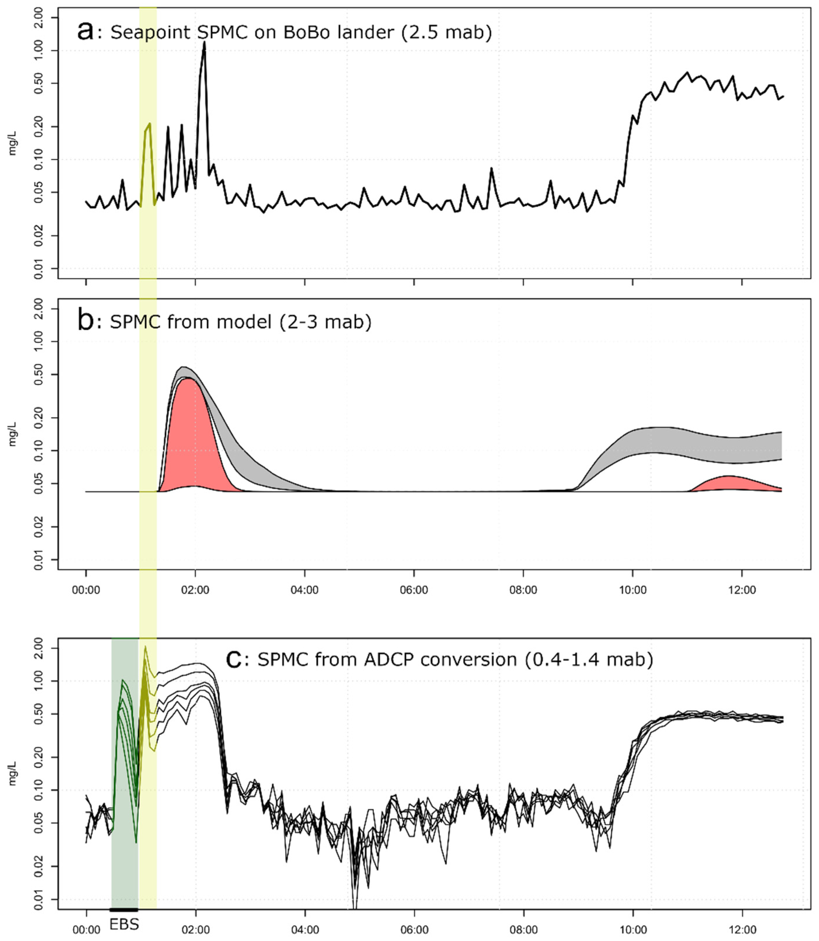
The EBS disturbed the seafloor resulting in mobilisation and partial resuspension and an associated increase of the SPMC in the bottom water. The EBS-SPMC was on average 6.4 mg/L—thus easily 100 times higher than the background SPMC. On the BoBo lander (station #11_BoBo-lander-1), the Seapoint captured the SPMC increases representing the EBS plume, manifested in two events separated in time by 7.5 h (
Figure 7a). The first SPM event (E1) that lasted for 1.7 h consisted of spiky but significant increases whereas the second event (E2) corresponds to a rather consistent SPMC of 0.5 mg/L over 3.4 h. During both events, the SPMC was significantly higher than the background but in general remained relatively low. E2, which was only partially recorded because the BoBo lander was retrieved before it had ended, lasted longer than the first, likely because of the tide reversal happening at that time.
The ADCP-SPMC during E1 shows a distinct vertical gradient with values of 1.0–1.5 mg/L at 0.5 mab, decreasing to 0.2–0.6 mg/L at 1.5 mab. The spikiness of the data as seen in the Seapoint SPMC is not present in the ADCP-SPMC, mainly because the sample volume of the acoustic backscatter is larger than the one of the Seapoint. Additionally, the ADCP average includes 50 samples, 10 times more than the Seapoint.
The ADCP-SPMC during E2 reveals a uniform vertical distribution of SPM, with concentration remaining almost constant over time at about 0.5 mg/L, similar to what is measured by the Seapoint.
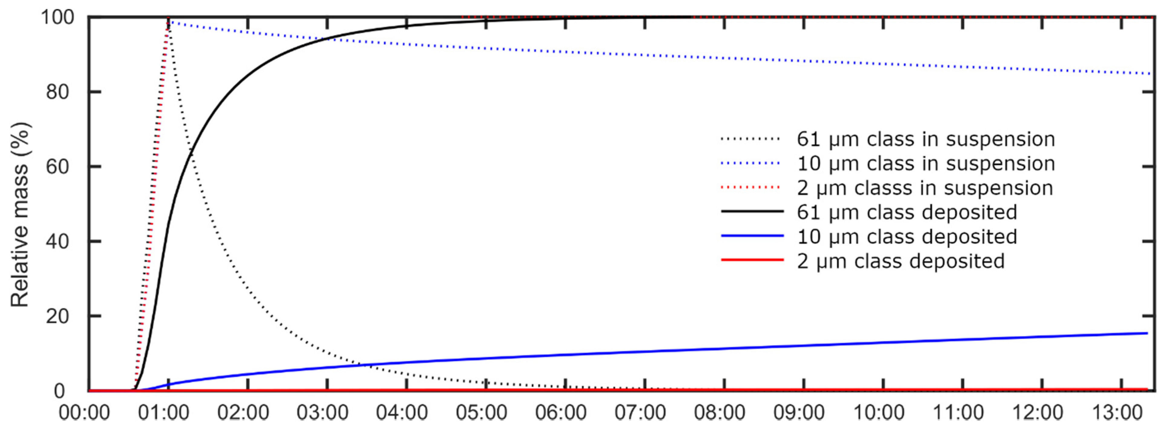
The model simulation of SPMC for the different classes reveals a rather fast deposition of 61 µm class with 95% deposited after about 3 h after the 20 min EBS disturbance stopped (
Figure 8). In addition, 10 µm class (d50) and 2 µm class (d10) remain in suspension for a much longer time, resp., 15% and 0.41% were deposited after 12 h. The simulated time series of 2 µm class SPMC for the BoBo location, shown in
Figure 8, reproduces both events E1 and E2, in agreement with what the Seapoint at 2.5 mab in the BoBo lander has measured. The timing of E2 and the SPMC concentration during E2 are somewhat off: lower SPMC and about 1 h offset. The influence of plume release height and seabed topography on plume dispersion was assessed by running different model simulations: plume release height at 0–1 mab vs. 1–2 mab, and actual bathymetry vs. flat bathymetry. The release height set at 1–2 mab (upper bound line of grey-filled curve in
Figure 7b) produces higher SPMC at 2–3 mab, especially during E2. The red-filled curve refers to SPMC simulated for a flat bathymetry, the grey-filled curve results from implementing the study area bathymetry. With and without realistic bathymetry, the model produces differences in both SPMC and timing for the second event mainly.
Unintentionally produced peaks in the acoustic backscatter of the ADCP from station #11_BoBo-lander-1 are likely related to underwater noise created by towing the EBS (
Figure 7, the 20 min window marked in green), as this peak matches in time of the actual EBS being towed over the seafloor. This acoustic peak was not recorded by the Seapoint as an increase in SPM concentrations. The second and shorter peak in acoustic backscatter can probably be explained by the action of EBS cable swiping over the seafloor preparatory towing (peak marked with yellow). The latter peak was now recorded by the Seapoint. Both peaks were not reproduced by the model.
4. Discussion
The main objective of the study is to assess the fate of a plume associated with a human induced seafloor disturbance in the deep-sea and to estimate the duration and geographical spreading of the suspended particles. For this, we combined optical and acoustic backscatter data, seafloor sediment characteristics and the results of a sediment transport model. Plume behaviour is mainly related to the hydrodynamics and the sediment characteristics, such as horizontal and vertical current velocities, flocculation potential, settling velocity, erodibility and SPMC. The synthesis between model results, in situ data and sediment characteristics deliver important insight into the fate of a sediment plume in the deep-sea.
In this way, we can thoroughly investigate the increases in SPMC due to man-made erosion of the seafloor. We will focus in the discussion on the erodibility, the settling and the transport of sediment particles and the influence of the seafloor topography to understand how the plume evolves over time.
4.1. Erodibility of the DISCOL Sediments
The EBS eroded the top layer in which Mn-nodules typically occur [
49]. The seafloor sediment erodibility is nevertheless mainly related to the particle size distribution of the sediment and particularly to the mud fraction (<63 µm; 80–95% in the samples) that increases the cohesiveness of the seafloor [
50,
51]. However, mechanical erosion of the top layer expressed as shear strength is low (0.1 kPa), unlike the underlying consolidated sediments which have a higher shear strength of up to 3–5 kPa [
14].
Sediment erosion by bottom currents can be excluded due to the weak bottom shear stresses exerted by the currents. Bottom shear stresses of at least 0.05–0.1 Pa are required to entrain the not-consolidated fluffy layer at the sediment–water interface (e.g., [
52,
53]. In this respect the plough marks from 1989, still well visible in 2015 [
24], indicating an absence of any significant sediment transport in the area. Only during the passage of surface meso-scale eddies and their associated energy transfer towards the seafloor weeks later, current speeds may surpass thresholds for sediment entrainment [
18,
20,
54], and even more for freshly deposited SPM [
17] days or weeks after mining. The freshly deposited sediments could thus be a reservoir of erodible sediments that will result in regular resuspension of these layers. Increase of turbidity associated with mining activities could thus occur long after the activity itself.
No natural seafloor erosion, due to weak currents/bottom shear stresses occurred during the time of observation that could have been the origin of the second SPM event seen in Seapoint and ADCP data of station #11_BoBo-lander-1. In addition, we have no field observation showing that the SPM plume was deposited and re-suspended before the second event (E2), only the model that informs us (at least for 2 and 10 µm classes) that the SPM plume continuously remained in suspension with little sedimentation (mainly 61 µm class) over the course of the measurement with BoBo sensors.
4.2. Flocculation of the SPM from Eroded Seafloor
Sedimentation may be enhanced by flocculation processes, as studied in different marine environments worldwide (e.g., [
55,
56,
57,
58]). In principle, flocculation depends on several local environmental conditions, such as turbulence, cation concentration, SPMC, mineral composition, organic matter (OM) concentration and composition and microorganism [
59,
60,
61,
62,
63]. The high amounts of clay minerals as smectite favours the cohesiveness of the sediments and thus supports a high flocculation potential. The cation concentrations are high and well above the threshold for salinity induced flocculation and the OM content (about 1%) measured in the sediment samples was low and most probably related to the organic carbon compounds trapped in the interlayer of the clay minerals [
64] such that flocculation in the study area is, above all, controlled by the mineral composition and the SPMC, and the hydrodynamic conditions. Particle composition, cations and presence of sticky OM affect the stickiness, which is important in determining what happens when particles react with each other during flocculation [
59].
4.3. EBS Plume SPMC and Evolution
From AUV and ROV observations [
49], the EBS left a 2.4 m wide scour mark of 5 cm depth and deeper with big lumps of muddy sediment at both sides of the track. A towing speed of 0.62 m/s thus implies 0.07 m
3 of wet sediment displaced per second; by far, most of it was only pushed aside and was not suspended into the water column. For the calculation of the corresponding weight of sediment particles that is mobilised, a specific mass of 2500 kg/m
3 for the sediments has been assumed. According to [
65], sediment porosity for the DISCOL area is 0.90. The total weight of dry sediment displacement rate by the EBS was estimated to 18.6 kg/s (most just pushed aside). The release rate into the water column used in the model simulation is 0.142 kg/s suggesting that less than 1% (0.8%) of the mobilised sediment eventually comes into suspension, for 5 cm deep scour marks.
The SPMC during the disturbance (measured directly on the EBS) was on average 6.4 mg/L at 1 mab (
Figure 6b), rapidly decreasing with time as the plume passed the BoBo location (after 15 min: about 1.5 mg/L, and after 9 h: 0.5 mg/L. During most of the time of the plume dispersal, SPMC and turbulence (G = 0.25 1/s) were too low and not favourable for aggregation (due to differential settling) [
17,
47,
59,
66]. The tidal current advected the plume first in a southward direction followed by a displacement in north-eastward direction (
Figure 9 and
Figure 10). The plume dispersion is thus only determined by the ambient current regime. The early far field E1 is thus characterised by higher SPMC, with distinct gradient of increasing SPMC towards the seafloor whereas E2 (later far field) is characterised by a lower SPMC, uniformly distributed (better mixed and thus more homogeneous and spread out than E1) in the lower 2.5 mab and remaining constant over at least 3 h. The SPMC during these events were up to 10 times (E2) and 100 times (E1) higher than the natural background SPMC.
From the model (
Figure 8), only about 0.41% of the slow settling 2 µm class (and 15% for 10 µm class) was settled by the end of the measurements (total duration of 12 h) implying that the plume may have continued to exist for about 121 days for 2 µm class (3.3 days for 10 µm class) assuming similar hydrodynamic conditions. The plume trajectory, and thus expanse of the plume, is controlled by the tidal and residual current and the release height. The plume displacement for a residence time of 121 and 3.3 days is estimated to be approximately 436 and 12 km, respectively. As the SPM is slowly settling and the concentration is generally low; the thickness of the deposited particles is about the same as for 2 µm and 10 µm class particle itself; this is not detectable in imagery.
4.4. The Role of Seafloor Topography
During E2, the modelled SPMC at 2–3 mab is 0.1 mg/L, and thus lower than the measured SPMC. The reason for this might be that the horizontal bathymetric resolution is not fine enough to capture all small-scale seafloor topography and the associated vertical current components. As a result, the SPM plume height is not fully resolved by the model. Having high resolution bathymetry for simulations seems to be crucial as the terrain morphology controls the often-subtle vertical current components defining either the plume to remain in suspension or not.
Figure 7b includes the simulation of the SPM plume for the 2 µm class when considering a flat bathymetry. There is a reduced upward presence of the SPM plume, as there is no vertical shear between the horizontal velocities.
5. Conclusions
Field observation and numerical model simulation of small-scale plume experiments provide new insights for realistic predictions of how sediment plumes generated by mining operations will be transported through the ocean. They are also helpful for designing future monitoring set-ups, based on the local hydrodynamic and bathymetric conditions.
Our field observations and numerical simulation of deep-sea sediment transport indicated that tides are a significant component in deep-sea suspended sediment transport in the Peru Basin and elsewhere. Future exploitation of polymetallic nodules will be performed with much larger seabed crawlers that will release sediments at a height of several meters (5–6 m) above the seafloor, and this is in much higher quantities than in our small scale EBS experiment [
67]. Similar as in our small-scale experiment, the coarser fraction in these industrial plumes will settle quickly (within hours). However, different from our experiment, flocculation processes will probably occur as the SPMC will be much higher. Part of the fine fraction will thus aggregate to form larger flocs, resulting in a faster settling. However, a slowly settling fine fraction will remain, similar as in our experiment, resulting in far field effects that may cover larger areas, depending on the initial concentration of this fine hardly settling fraction.
Our model results show that the effect of bathymetry on the current velocity changes the vertical dispersion of the plume above the seafloor and thus the deposition of particles. Therefore, to prevent significant ecological impact of deep-sea mining in the far-field area, a precise analysis of seafloor slopes is of great importance and should be further evaluated using numerical simulations. This has already been pointed out by [
68]. Depending on the tidal currents, direction, and bathymetry, a best time window could be chosen to minimize the dispersion of the plume and thus to reduce the environmental impact of mining.
Author Contributions
Conceptualization, M.B., H.d.S., B.G. and M.F.; methodology, M.B., K.P. and B.G.; validation, K.P.; formal analysis, M.B.; investigation, M.B. and K.P.; writing—original draft preparation, M.B.; writing—review and editing, K.P., H.d.S., B.G., M.F. and J.G.; visualization, M.B.; supervision, H.d.S. and M.F.; project administration, H.d.S. and M.B. acted as the lead author and incorporated ideas and individual text contributions from the co-authors. K.P. implemented the model and performed the simulations. All authors have read and agreed to the published version of the manuscript.
Funding
Ship time was funded by the German Federal Ministry of Education and Research through the “MiningImpact” project (grant 03F0707A-G of the Joint Programming Initiative of Healthy and Productive Seas and Oceans (JPIO)). The deployment of the equipped bottom landers, EBS and MUC was achieved with funding by the Dutch Research Council NWO, grant 856.14.003; the German BMBF (grant 03F0707A-G); the Belgian funding agency “Belgian Science Policy Office” (grants BR14/MA/JPI-DEEPSEA1 and BR15/MA/JPI-DEEPSEA2).
Institutional Review Board Statement
Not applicable.
Informed Consent Statement
Not applicable.
Data Availability Statement
Acknowledgments
We would like to thank the captain and the crew of the RV Sonne for all their support during SO242. Lieven Naudts was responsible for the RBINS funding acquisition and project administration. The mineralogical and grain size analysis were performed by QMineral (
https://www.qmineral.com/, accessed on 12 November 2021). The authors also would like to thank the reviewers for their constructive comments.
Conflicts of Interest
The authors declare no conflict of interest.
Appendix A
Table A1.
Quantitative bulk mineralogical compositions of the samples in weight percentages (wt%).
Table A1.
Quantitative bulk mineralogical compositions of the samples in weight percentages (wt%).
| | 119_MUC-31 | 34_MUC-6 | 70_MUC-17 |
|---|
| | 0–5 cm | 5–15 cm | 0–5 cm | 5–15 cm | 0–5 cm | 5–15 cm |
|---|
| Quartz | 6.0 | 7.8 | 7.8 | 6.8 | 6.1 | 6.9 |
| K-spar | 2.6 | 3.5 | 3.9 | 3.7 | 2.7 | 2.7 |
| Plagioclase | 5.7 | 6.0 | 7.0 | 5.4 | 5.5 | 5.2 |
| Calcite | 0.0 | 1.7 | 1.5 | 2.0 | 2.0 | 4.2 |
| Dolomite | 0.5 | 0.4 | 0.6 | 0.3 | 0.4 | 0.3 |
| Siderite | 0.0 | 0.0 | 0.1 | 0.2 | 0.2 | 0.3 |
| Gypsum | 0.0 | 0.0 | 0.6 | 0.2 | 0.1 | 0.3 |
| Barite | 1.9 | 1.8 | 2.3 | 1.6 | 1.5 | 2.1 |
| Anatase | 0.0 | 0.3 | 0.8 | 0.1 | 0.0 | 0.3 |
| Halite | 5.4 | 4.6 | 12.9 | 3.0 | 4.2 | 4.6 |
| Apatite | 0.9 | 1.2 | 0.6 | 0.6 | 0.5 | 0.4 |
| | 23.0 | 27.3 | 38.0 | 23.9 | 23.3 | 27.2 |
| Kaolinite | 0.7 | 1.0 | 4.3 | 2.8 | 2.0 | 1.7 |
| Chlorite | 0.0 | 0.0 | 0.4 | 0.1 | 0.6 | 0.5 |
| 2:1 clays | 40.5 | 39.8 | 27.5 | 47.2 | 39.3 | 38.0 |
| | 41.2 | 40.8 | 32.1 | 50.1 | 42.0 | 40.2 |
| Amorphous | 35.8 | 31.9 | 29.9 | 26.0 | 34.8 | 32.6 |
Table A2.
Quantitative chemical composition of the samples in wt%.
Table A2.
Quantitative chemical composition of the samples in wt%.
| Analyte Symbol | SiO2 | Al2O3 | Fe2O3(T) | MnO | MgO | CaO | Na2O | K2O | TiO2 | P2O5 |
| Unit Symbol | % | % | % | % | % | % | % | % | % | % |
| Detection Limit | 0.01 | 0.01 | 0.01 | 0.001 | 0.01 | 0.01 | 0.01 | 0.01 | 0.001 | 0.01 |
| Analysis Method | FUS-ICP | FUS-ICP | FUS-ICP | FUS-ICP | FUS-ICP | FUS-ICP | FUS-ICP | FUS-ICP | FUS-ICP | FUS-ICP |
| 119_MUC-31 0–5 cm | 46.72 | 9.55 | 5.08 | 3.323 | 2.46 | 1.45 | 6.58 | 1.62 | 0.39 | 0.34 |
| 119_MUC-31 5–15 cm | 41.9 | 8.46 | 4.45 | 2.153 | 2.11 | 2.01 | 4.65 | 1.41 | 0.347 | 0.27 |
| 34_MUC-6 0–5 cm | 45.84 | 9.86 | 4.76 | 1.733 | 2.36 | 1.78 | 6.53 | 1.63 | 0.372 | 0.31 |
| 34_MUC-6 5–15 cm | 51.95 | 10.49 | 5.13 | 1.676 | 2.29 | 3.01 | 4.26 | 1.73 | 0.405 | 0.33 |
| 70_MUC-17 0–5 cm | 50.48 | 10.45 | 5.09 | 1.858 | 2.37 | 2.16 | 4.93 | 1.73 | 0.408 | 0.35 |
| 70_MUC-17 5–15 cm | 40.47 | 8.92 | 4.19 | 0.667 | 2 | 3.71 | 4.66 | 1.5 | 0.329 | 0.25 |
| Analyte Symbol | Ba | Sr | Y | Sc | Zr | Be | V | | | |
| Unit Symbol | ppm | ppm | ppm | ppm | ppm | ppm | ppm | | | |
| Detection Limit | 2 | 2 | 1 | 1 | 2 | 1 | 5 | | | |
| Analysis Method | FUS-ICP | FUS-ICP | FUS-ICP | FUS-ICP | FUS-ICP | FUS-ICP | FUS-ICP | | | |
| 119_MUC-31 0–5 cm | 7616 | 358 | 66 | 21 | 112 | 2 | 108 | | | |
| 119_MUC-31 5–15 cm | 6418 | 319 | 54 | 18 | 100 | 1 | 91 | | | |
| 34_MUC-6 0–5 cm | 7504 | 367 | 60 | 20 | 105 | 2 | 106 | | | |
| 34_MUC-6 5–15 cm | 8076 | 402 | 66 | 22 | 117 | 2 | 113 | | | |
| 70_MUC-17 0–5 cm | 8211 | 396 | 69 | 22 | 114 | 2 | 117 | | | |
| 70_MUC-17 5–15 cm | 6437 | 346 | 50 | 18 | 99 | 1 | 87 | | | |
| Analyte Symbol | C-Total | Total S | LOI | Total | | | | | | |
| Unit Symbol | % | % | % | % | | | | | | |
| Detection Limit | 0.01 | 0.01 | | 0.01 | | | | | | |
| Analysis Method | CS | CS | FUS-ICP | FUS-ICP | | | | | | |
| 119_MUC-31 0–5 cm | 0.74 | 0.27 | 18.74 | 77.5 | | | | | | |
| 119_MUC-31 5–15 cm | 0.88 | 0.29 | 25.53 | 67.77 | | | | | | |
| 34_MUC-6 0–5 cm | 0.75 | 0.36 | 23.69 | 98.87 | | | | | | |
| 34_MUC-6 5–15 cm | 1.01 | 0.3 | 17.68 | 98.95 | | | | | | |
| 70_MUC-17 0–5 cm | 0.89 | 0.33 | 19.45 | 99.27 | | | | | | |
| 70_MUC-17 5–15 cm | 1.05 | 0.25 | 32.44 | 99.12 | | | | | | |
Table A3.
Quantitative clay composition of the <2 µm fraction of pre-treated samples in wt%.
Table A3.
Quantitative clay composition of the <2 µm fraction of pre-treated samples in wt%.
| | Smectite | I/S R0 | Illite | Kaolinite | K/S R0 | Chlorite |
|---|
| 119_MUC-31 0–5 cm | 44.6 | 19.8 | 19.9 | 3.7 | 10.5 | 1.5 |
| 119_MUC-31 5–15 cm | 46.7 | 17.2 | 21.2 | 3.8 | 9.5 | 1.6 |
| 34_MUC-6 0–5 cm | 45.9 | 21.4 | 19.0 | 4.9 | 6.7 | 2.1 |
| 34_MUC-6 5–15 cm | 46.7 | 24.5 | 17.2 | 3.8 | 6.2 | 1.6 |
| 70_MUC-17 0–5 cm | 49.7 | 23.5 | 14.9 | 3.6 | 6.1 | 2.2 |
| 70_MUC-17 5–15 cm | 48.0 | 20.2 | 19.2 | 3.9 | 5.8 | 2.9 |
Table A4.
Quantitative determination of organic carbon after combustion of the samples.
Table A4.
Quantitative determination of organic carbon after combustion of the samples.
| IR | OM % |
|---|
| 119_MUC-31 0–5 cm | 0.99 |
| 119_MUC-31 5–15 cm | 1.08 |
| 34_MUC-6 0–5 cm | 0.93 |
| 34_MUC-6 5–15 cm | 0.77 |
| 70_MUC-17 0–5 cm | 1.00 |
| 70_MUC-17 5–15 cm | 0.70 |
Appendix B
Figure A1.
Plot of the periodogram of the total current speed (1 mab) from the BoBo lander stations.
Figure A1.
Plot of the periodogram of the total current speed (1 mab) from the BoBo lander stations.
References
- Rateev, M.A.; Sadchikova, T.A.; Shabrova, V.P. Clay Minerals in Recent Sediments of the World Ocean and Their Relation to Types of Lithogenesis. Lithol. Miner. Resour. 2008, 43, 125–135. [Google Scholar] [CrossRef]
- Glasby, G.P. Mineralogy, Geochemistry, and Origin of Pacific Red Clays: A Review. N. Z. J. Geol. Geophys. 1991, 34, 167–176. [Google Scholar] [CrossRef]
- Haeckel, M.; König, I.; Riech, V.; Weber, M.E.; Suess, E. Pore Water Profiles and Numerical Modelling of Biogeochemical Processes in Peru Basin Deep-Sea Sediments. Deep-Sea Res. Part II 2001, 48, 3713–3736. [Google Scholar] [CrossRef]
- Chester, R. Marine Geochemistry by Roy Chester. Unwin Hyman, London, 1990. No of Pages: 698. Price £34.95 (Paperback); £90.00 (Hardback). ISBN 0 045 51109 8 (Paperback); 0 045 511 08 X (Hardback). Geol. J. 1993, 28, 96–97. [Google Scholar] [CrossRef]
- Fagel, N. Chapter Four Clay Minerals, Deep Circulation and Climate. In Developments in Marine Geology; Elsevier: Amsterdam, The Netherlands, 2007; Volume 1, pp. 139–184. ISBN 978-0-444-52755-4. [Google Scholar]
- Inoue, A. Formation of Clay Minerals in Hydrothermal Environments. In Origin and Mineralogy of Clays; Velde, B., Ed.; Springer: Berlin/Heidelberg, Germany, 1995; pp. 268–329. ISBN 978-3-642-08195-8. [Google Scholar]
- Lal, D. The Oceanic Microcosm of Particles: Suspended Particulate Matter, about 1 g in 100 Tons of Seawater, Plays a Vital Role in Ocean Chemistry. Science 1977, 198, 997–1009. [Google Scholar] [CrossRef] [PubMed]
- Alldredge, A.L.; Silver, M.W. Characteristics, Dynamics and Significance of Marine Snow. Prog. Oceanogr. 1988, 20, 41–82. [Google Scholar] [CrossRef]
- Thiel, H.; Schriever, G. Deep-Sea Mining, Environmental Impact and the DISCOL Project. Ambio 1990, 19, 245–250. [Google Scholar]
- Lavelle, J.W.; Ozturgut, E.; Baker, E.T.; Swift, S.A. Discharge and Surface Plume Measurements during Manganese Nodule Mining Tests in the North Equatorial Pacific. Mar. Environ. Res. 1982, 7, 51–70. [Google Scholar] [CrossRef]
- Ozturgut, E.; Lavelle, J.W.; Burns, R.E. Chapter 15 Impacts of Manganese Nodule Mining on the Environment: Results from Pilot-Scale Mining Tests in the North Equatorial Pacific. In Elsevier Oceanography Series; Elsevier: Amsterdam, The Netherlands, 1981; Volume 27, pp. 437–474. ISBN 978-0-444-41855-5. [Google Scholar]
- Klein, H. Near-Bottom Currents in the Deep Peru Basin, DISCOL Experimental Area. Dtsch. Hydrogr. Z. 1993, 45, 31–42. [Google Scholar] [CrossRef]
- Klein, H. Near-Bottom Currents and Bottom Boundary Layer Variability over Manganese Nodule Fields in the Peru Basin, Se-Pacific. Dtsch. Hydrogr. Z. 1996, 48, 147–160. [Google Scholar] [CrossRef]
- Grupe, B.; Becker, H.J.; Oebius, H.U. Geotechnical and Sedimentological Investigations of Deep-Sea Sediments from a Manganese Nodule Field of the Peru Basin. Deep-Sea Res. Part II 2001, 48, 3593–3608. [Google Scholar] [CrossRef]
- Thiel, H. Evaluation of the Environmental Consequences of Polymetallic Nodule Mining Based on the Results of the TUSCH Research Association. Deep-Sea Res. Part II Top. Stud. Oceanogr. 2001, 48, 3433–3452. [Google Scholar] [CrossRef]
- Jones, D.O.B.; Durden, J.M.; Murphy, K.; Gjerde, K.M.; Gebicka, A.; Colaço, A.; Morato, T.; Cuvelier, D.; Billett, D.S.M. Existing Environmental Management Approaches Relevant to Deep-Sea Mining. Mar. Policy 2019, 103, 172–181. [Google Scholar] [CrossRef]
- Gillard, B.; Purkiani, K.; Chatzievangelou, D.; Vink, A.; Iversen, M.H.; Thomsen, L. Physical and Hydrodynamic Properties of Deep Sea Mining-Generated, Abyssal Sediment Plumes in the Clarion Clipperton Fracture Zone (Eastern-Central Pacific). Elem. Sci. Anthr. 2019, 7, 5. [Google Scholar] [CrossRef] [Green Version]
- Aleynik, D.; Inall, M.E.; Dale, A.; Vink, A. Impact of Remotely Generated Eddies on Plume Dispersion at Abyssal Mining Sites in the Pacific. Sci. Rep. 2017, 7, 16959. [Google Scholar] [CrossRef] [PubMed] [Green Version]
- Chen, H.; Zhang, W.; Xie, X.; Ren, J. Sediment Dynamics Driven by Contour Currents and Mesoscale Eddies along Continental Slope: A Case Study of the Northern South China Sea. Mar. Geol. 2019, 409, 48–66. [Google Scholar] [CrossRef]
- Purkiani, K.; Paul, A.; Vink, A.; Walter, M.; Schulz, M.; Haeckel, M. Evidence of Eddy-Related Deep-Ocean Current Variability in the Northeast Tropical Pacific Ocean Induced by Remote Gap Winds. Biogeosciences 2020, 17, 6527–6544. [Google Scholar] [CrossRef]
- Purkiani, K.; Gillard, B.; Paul, A.; Haeckel, M.; Haalboom, S.; Greinert, J.; de Stigter, H.; Hollstein, M.; Baeye, M.; Vink, A.; et al. Numerical Simulation of Deep-Sea Sediment Transport Induced by a Dredge Experiment in the Northeastern Pacific Ocean. Front. Mar. Sci. 2021, 8, 719463. [Google Scholar] [CrossRef]
- Gausepohl, F.; Hennke, A.; Schoening, T.; Köser, K.; Greinert, J. Scars in the Abyss: Reconstructing Sequence, Location and Temporal Change of the 78 Plough Tracks of the 1989 DISCOL Deep-Sea Disturbance Experiment in the Peru Basin. Biogeosciences 2020, 17, 1463–1493. [Google Scholar] [CrossRef] [Green Version]
- Wiedicke, M.H.; Weber, M.E. Small-Scale Variability of Seafloor Features in the Northern Peru Basin: Results from Acoustic Survey Methods. Mar. Geophys. Res. 1996, 18, 507–526. [Google Scholar] [CrossRef]
- Greinert, J. RV Sonne Fahrtbericht/Cruise Report SO242-1 [SO242/1]: JPI Oceans Ecological Aspects of Deep-Sea Mining, DISCOL Revisited, Guayaquil—Guayaquil (Equador), 28.07.-25.08.2015; GEOMAR Report; GEOMAR Helmholtz-Zentrum für Ozeanforschung: Kiel, Germany, 2015; p. 290. [Google Scholar]
- Weber, M.E.; Wiedicke, M.; Riech, V.; Erlenkeuser, H. Carbonate Preservation History in the Peru Basin: Paleoceanographic Implications. Paleoceanography 1995, 10, 775–800. [Google Scholar] [CrossRef]
- Visbeck, M.; Gelpke, N. (Eds.) Marine Resources—Opportunities and Risks; World Ocean Review [Englische Ausgabe]; Maribus: Hamburg, Germany, 2014; ISBN 978-3-86648-221-0. [Google Scholar]
- Von Stackelberg, U. Growth History of Manganese Nodules and Crusts of the Peru Basin. Geol. Soc. Lond. Spec. Publ. 1997, 119, 153–176. [Google Scholar] [CrossRef]
- Weber, M.E.; von Stackelberg, U.; Marchig, V.; Wiedicke, M.; Grupe, B. Variability of Surface Sediments in the Peru Basin: Dependence on Water Depth, Productivity, Bottom Water Flow, and Seafloor Topography. Mar. Geol. 2000, 163, 169–184. [Google Scholar] [CrossRef]
- Rietveld, H.M. A Profile Refinement Method for Nuclear and Magnetic Structures. J. Appl. Crystallogr. 1969, 2, 65–71. [Google Scholar] [CrossRef]
- Scarlett, N.V.Y.; Madsen, I.C. Quantification of Phases with Partial or No Known Crystal Structures. Powder Diffr. 2006, 21, 278–284. [Google Scholar] [CrossRef]
- van Weering, T.; Thomsen, L.; Heerwaarden, J.; Koster, B.; Viergutz, T. A Seabed Lander and New Techniques for Long Term in Situ Study of Deep-Sea near Bed Dynamics. Sea Technol. 2000, 41, 17–27. [Google Scholar]
- Pfannkuche, O.; Linke, P. GEOMAR Landers as Long-Term Deep-Sea Observatories Applications and Developments of Lander Technology in Opera- Tional Oceanography. Sea Technol. 2003, 44, 50–55. [Google Scholar]
- Baker, E.T.; Tennant, D.A.; Feely, R.A.; Lebon, G.T.; Walker, S.L. Field and Laboratory Studies on the Effect of Particle Size and Composition on Optical Backscattering Measurements in Hydrothermal Plumes. Deep-Sea Res. Part I Oceanogr. Res. Pap. 2001, 48, 593–604. [Google Scholar] [CrossRef]
- Downing, J. Twenty-Five Years with OBS Sensors: The Good, the Bad, and the Ugly. Cont. Shelf Res. 2006, 26, 2299–2318. [Google Scholar] [CrossRef]
- Taylor, J.A.; Jonas, A.M. Maximising Data Return: Towards a Quality Control Strategy for Managing and Processing TRDI ADCP Data Sets from Moored Instrumentation. In Proceedings of the 2008 IEEE/OES 9th Working Conference on Current Measurement Technology, Charleston, SC, USA, 17–19 March 2008; pp. 80–88. [Google Scholar]
- Alessi, C.A.; Beardsley, R.C.; Limeburner, R.; Rosenfeld, L.K. Introduction to the CODE-2 Moored Array and Large-Scale Data Report; WHOI: Falmouth, MA, USA, 1985; p. 234. [Google Scholar]
- Nowell, A.R.; Jumars, P.A. Flumes: Theoretical and Experimental Considerations for Simulation of Benthic Environments. Oceanogr. Mar. Biol. 1987, 25, 91–112. [Google Scholar]
- Schlichting, H. Boundary Layer Theory, 6th ed.; McGraw-Hill: New York, NY, USA, 1962. [Google Scholar]
- Dyer, K.R.; Manning, A.J. Observation of the Size, Settling Velocity and Effective Density of Flocs, and Their Fractal Dimensions. J. Sea Res. 1999, 41, 87–95. [Google Scholar] [CrossRef]
- Berhane, I.; Sternberg, R.W.; Kineke, G.C.; Milligan, T.G.; Kranck, K. The Variability of Suspended Aggregates on the Amazon Continental Shelf. Cont. Shelf Res. 1997, 17, 267–285. [Google Scholar] [CrossRef]
- Safak, I.; Allison, M.A.; Sheremet, A. Floc Variability under Changing Turbulent Stresses and Sediment Availability on a Wave Energetic Muddy Shelf. Cont. Shelf Res. 2013, 53, 1–10. [Google Scholar] [CrossRef]
- Sahin, C.; Verney, R.; Sheremet, A.; Voulgaris, G. Acoustic Backscatter by Suspended Cohesive Sediments: Field Observations, Seine Estuary, France. Cont. Shelf Res. 2017, 134, 39–51. [Google Scholar] [CrossRef] [Green Version]
- Deines, K.L. Backscatter Estimation Using Broadband Acoustic Doppler Current Profilers. In Proceedings of the IEEE Sixth Working Conference on Current Measurement (Cat. No. 99CH36331), San Diego, CA, USA, 13 March 1999; pp. 249–253. [Google Scholar]
- Brenke, N. An Epibenthic Sledge for Operations on Marine Soft Bottom and Bedrock. Mar. Technol. Soc. J. 2005, 39, 10–21. [Google Scholar] [CrossRef]
- Marshall, J.; Adcroft, A.; Hill, C.; Perelman, L.; Heisey, C. A Finite-Volume, Incompressible Navier Stokes Model for Studies of the Ocean on Parallel Computers. J. Geophys. Res. 1997, 102, 5753–5766. [Google Scholar] [CrossRef] [Green Version]
- Marshall, J.; Hill, C.; Perelman, L.; Adcroft, A. Hydrostatic, Quasi-Hydrostatic, and Nonhydrostatic Ocean Modeling. J. Geophys. Res. 1997, 102, 5733–5752. [Google Scholar] [CrossRef]
- Muñoz-Royo, C.; Peacock, T.; Alford, M.H.; Smith, J.A.; Le Boyer, A.; Kulkarni, C.S.; Lermusiaux, P.F.J.; Haley, P.J.; Mirabito, C.; Wang, D.; et al. Extent of Impact of Deep-Sea Nodule Mining Midwater Plumes Is Influenced by Sediment Loading, Turbulence and Thresholds. Commun. Earth Environ. 2021, 2, 148. [Google Scholar] [CrossRef]
- Large, W.G.; McWilliams, J.C.; Doney, S.C. Oceanic Vertical Mixing: A Review and a Model with a Nonlocal Boundary Layer Parameterization. Rev. Geophys. 1994, 32, 363. [Google Scholar] [CrossRef] [Green Version]
- Martínez Arbizu, P.; Haeckel, M. RV Sonne Fahrtbericht/Cruise Report SO239: EcoResponse Assessing the Ecology, Connectivity and Resilience of Polymetallic Nodule Field Systems, Balboa (Panama) Manzanillo (Mexico) 11.03.-30.04.2015; GEOMAR Report; GEOMAR Helmholtz-Zentrum für Ozeanforschung: Kiel, Germany, 2015; p. 204. [Google Scholar]
- Le Hir, P.; Cayocca, F.; Waeles, B. Dynamics of Sand and Mud Mixtures: A Multiprocess-Based Modelling Strategy. Cont. Shelf Res. 2011, 31, S135–S149. [Google Scholar] [CrossRef] [Green Version]
- van Rijn, L.C. Unified View of Sediment Transport by Currents and Waves. I: Initiation of Motion, Bed Roughness, and Bed-Load Transport. J. Hydraul. Eng. 2007, 133, 649–667. [Google Scholar] [CrossRef] [Green Version]
- Butman, B.; Aretxabaleta, A.L.; Dickhudt, P.J.; Dalyander, P.S.; Sherwood, C.R.; Anderson, D.M.; Keafer, B.A.; Signell, R.P. Investigating the Importance of Sediment Resuspension in Alexandrium Fundyense Cyst Population Dynamics in the Gulf of Maine. Deep Sea Res. Part II Top. Stud. Oceanogr. 2014, 103, 79–95. [Google Scholar] [CrossRef] [Green Version]
- Thomsen, L.; Gust, G. Sediment Erosion Thresholds and Characteristics of Resuspended Aggregates on the Western European Continental Margin. Deep Sea Res. Part I Oceanogr. Res. Pap. 2000, 47, 1881–1897. [Google Scholar] [CrossRef]
- Dutkiewicz, A.; Judge, A.; Müller, R.D. Environmental Predictors of Deep-Sea Polymetallic Nodule Occurrence in the Global Ocean. Geology 2020, 48, 293–297. [Google Scholar] [CrossRef]
- Fettweis, M.; Baeye, M. Seasonal Variation in Concentration, Size, and Settling Velocity of Muddy Marine Flocs in the Benthic Boundary Layer: Seasonality of SPM Concentration. J. Geophys. Res. Oceans 2015, 120, 5648–5667. [Google Scholar] [CrossRef] [Green Version]
- Maggi, F. Biological Flocculation of Suspended Particles in Nutrient-Rich Aqueous Ecosystems. J. Hydrol. 2009, 376, 116–125. [Google Scholar] [CrossRef]
- Manning, A.J.; Langston, W.J.; Jonas, P.J.C. A Review of Sediment Dynamics in the Severn Estuary: Influence of Flocculation. Mar. Pollut. Bull. 2010, 61, 37–51. [Google Scholar] [CrossRef]
- Markussen, T.N.; Elberling, B.; Winter, C.; Andersen, T.J. Flocculated Meltwater Particles Control Arctic Land-Sea Fluxes of Labile Iron. Sci. Rep. 2016, 6, 24033. [Google Scholar] [CrossRef] [PubMed]
- Dyer, K.R. Sediment Processes in Estuaries: Future Research Requirements. J. Geophys. Res. 1989, 94, 14327. [Google Scholar] [CrossRef]
- Keyvani, A.; Strom, K. Influence of Cycles of High and Low Turbulent Shear on the Growth Rate and Equilibrium Size of Mud Flocs. Mar. Geol. 2014, 354, 1–14. [Google Scholar] [CrossRef]
- Lai, H.; Fang, H.; Huang, L.; He, G.; Reible, D. A Review on Sediment Bioflocculation: Dynamics, Influencing Factors and Modeling. Sci. Total Environ. 2018, 642, 1184–1200. [Google Scholar] [CrossRef] [PubMed]
- Mietta, F.; Chassagne, C.; Manning, A.J.; Winterwerp, J.C. Influence of Shear Rate, Organic Matter Content, PH and Salinity on Mud Flocculation. Ocean. Dyn. 2009, 59, 751–763. [Google Scholar] [CrossRef] [Green Version]
- Zhang, Y.; Liu, P.; Xiao, L.; Zhang, Y.; Yang, X.; Jiang, L. Experimental Study on Flocculation Effect of Tangential Velocity in a Cone-Plate Clarifier. Separations 2021, 8, 105. [Google Scholar] [CrossRef]
- Mayer, L.M. Relationships between Mineral Surfaces and Organic Carbon Concentrations in Soils and Sediments. Chem. Geol. 1994, 114, 347–363. [Google Scholar] [CrossRef]
- Haffert, L.; Haeckel, M.; de Stigter, H.; Janssen, F. Assessing the Temporal Scale of Deep-Sea Mining Impacts on Sediment Biogeochemistry. Biogeosciences 2020, 17, 2767–2789. [Google Scholar] [CrossRef]
- Berlamont, J.; Ockenden, M.; Toorman, E.; Winterwerp, J. The Characterisation of Cohesive Sediment Properties. Coast. Eng. 1993, 21, 105–128. [Google Scholar] [CrossRef] [Green Version]
- Oebius, H.U.; Becker, H.J.; Rolinski, S.; Jankowski, J.A. Parametrization and Evaluation of Marine Environmental Impacts Produced by Deep-Sea Manganese Nodule Mining. Deep-Sea Res. Part II Top. Stud. Oceanogr. 2001, 48, 3453–3467. [Google Scholar] [CrossRef]
- Peukert, A.; Schoening, T.; Alevizos, E.; Köser, K.; Kwasnitschka, T.; Greinert, J. Understanding Mn-Nodule Distribution and Evaluation of Related Deep-Sea Mining Impacts Using AUV-Based Hydroacoustic and Optical Data. Biogeosciences 2018, 15, 2525–2549. [Google Scholar] [CrossRef] [Green Version]
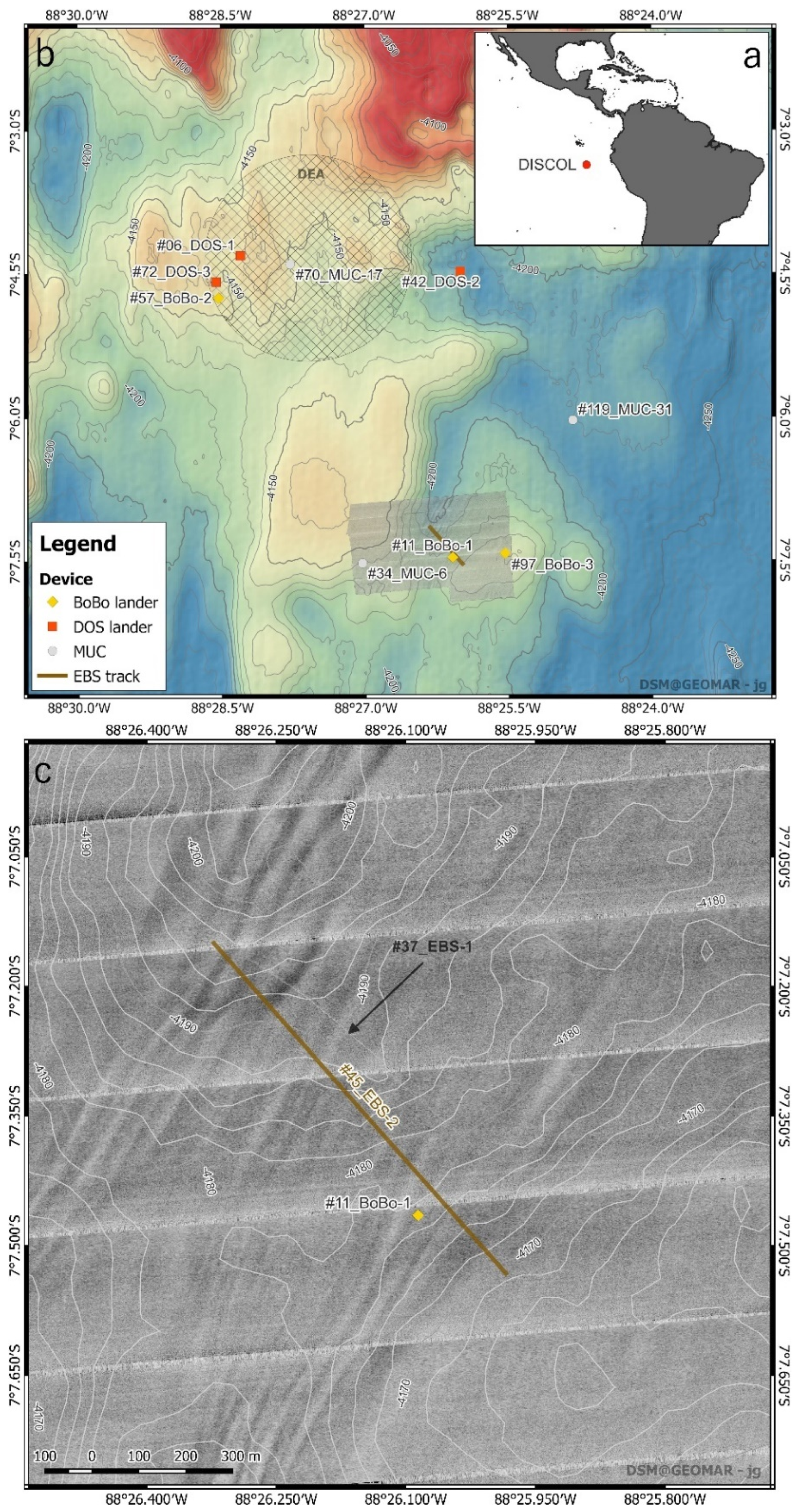
Figure 1.
(a) The location of the DISCOL (DEA, SE-Pacific Ocean). (b) Bathymetric map of DEA (ploughed in 1989) and surroundings. White circles are the MUC cores selected for sediment analysis. The yellow diamond symbols are the BoBo and DOS lander stations. The bathymetry obtained from the RV Sonne based EM122 12 kHz multibeam system in 2015 (SO242). Overlaid sidescan map (#41_AUV-5) of part of the reference area south where two EBS experiments (seafloor disturbing and associated sediment plume monitoring) took place in 2015. (c) A zoom in the sidescan map with the BoBo lander (yellow diamond) and visible fresh scour mark of the #37_EBS-1 track (indicated with black arrow), and the #45_EBS-2 track. Sidescan sonar (Edgetech) imagery (120 kHz) was realised from an autonomous underwater vehicle (AUV Abyss) at 30 m above the seafloor.
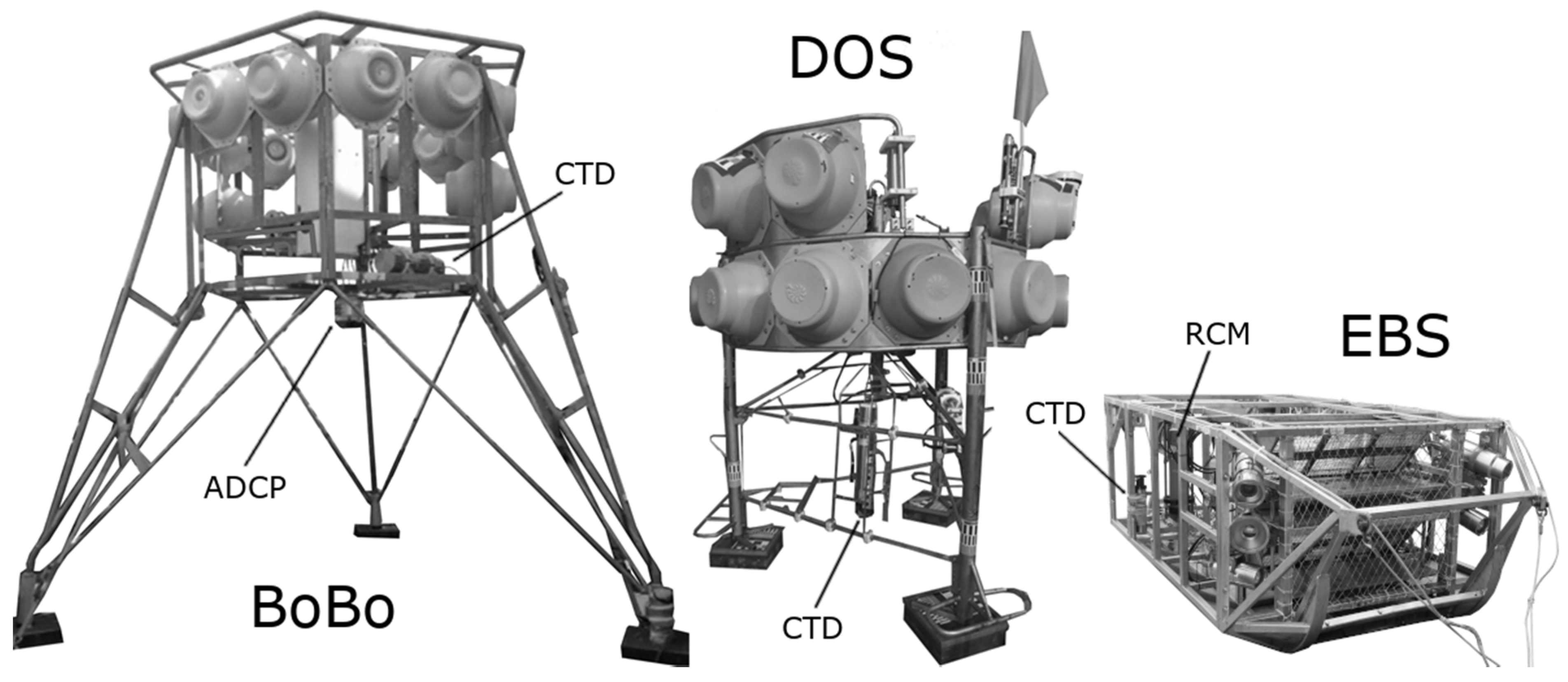
Figure 2.
An overview of the boundary layer monitoring devices used in this study. Left to right: Bottom Boundary Layer lander (BoBo) with CTD including a Seapoint turbidimeter at 2.5 mab and the downward ADCP current profiler at 2 mab; Deep-sea Observation System (DOS) with CTD including a Seapoint at 1 mab; Epi-benthic sledge (EBS) with CTD including a Seapoint at 0.5 mab and recording current meter (RCM) at 1 mab. The EBS towed by RV Sonne was used as the seafloor disturber.
Figure 3.
(
a) Seapoint FNU–SPMC linear relationship (R
2 = 0.98) using calibration suspensions prepared with surface sediments from multicore station #34_MUC-6 closest to the experiment site (
Figure 1). (
b) Linear relationship (R
2 = 0.75) between the acoustic backscatter from the Aanderaa recording current meter (RCM) and the natural logarithm of the Seapoint SPMC, both mounted on the EBS. The shaded band is a pointwise 95% confidence interval on the fitted line.
Figure 4.
The average particle size distribution (volume-based) of the non-prepared (black) and pre-treated surface sediment samples (red; disaggregation of flocculi, removal of carbonates, Mn-/Fe-oxides and Mn-/Fe-hydroxides).
Figure 4.
The average particle size distribution (volume-based) of the non-prepared (black) and pre-treated surface sediment samples (red; disaggregation of flocculi, removal of carbonates, Mn-/Fe-oxides and Mn-/Fe-hydroxides).
Figure 5.
(a) ADCP total current speed (1 mab) and (b) current direction (1 mab) from station 11_BoBo-1 and 57_BoBo-2. The residual data (grey lines) derived from the lowpass filtered meridional and longitudinal current components. (b) Current direction at 1 mab (black line) with the residual current direction (grey line). Vertical bar indicates the 20 min time interval of the #45_EBS-2 actual seafloor disturbance.
Figure 6.
(a) Boxplot of all SPM concentration (SPMC) data from all CTD-Seapoints from both BoBo (measured at 2.5 mab) and DOS (measured at 1 mab) landers; (b) the RCM-derived SPMC (measured at 1 mab) during the station #45_EBS-2 experiment. Data from the EBS Seapoint (with small FNU range) are not shown because that sensor was often saturated.
Figure 7.
(a) Time series of SPMC measured at 2.5 mab by the Seapoint sensor on the BoBo lander, during the EBS experiment on August 5th, 2015. The plume was detected twice (E1 and E2). The first peak marked by yellow shading was probably produced by the EBS towing cable sweeping over the seafloor. (b) Modelled SPMC time-series for the 2–3 mab vertical model grid cell corresponding to the position of the Seapoint sensor on BoBo. The grey and red shaded areas refer to the SPMC simulated while implementing the real bathymetry or assuming a horizontal seafloor, respectively. The lower and upper bounds of the shaded areas represent simulations for release heights of 0–1 mab and 1–2 mab, respectively. (c) Time series of SPMC derived from acoustic backscatter recorded with the downward-looking 1200 kHz RDI ADCP mounted on the BoBo lander, for 6 vertical depth bins centred, respectively, at 0.4, 0.6, 0.8, 1.0, 1.2 and 1.4 mab. The first peak in the ADCP-SPMC marked by green shading is related to the underwater noise created by towing the EBS (black line). Peaks produced by the towing cable and EBS noise are obviously not reproduced by the model simulation.
![Geosciences 12 00008 g007]()
Figure 8.
Percentage of deposition (solid line) and in suspension (dashed line) for each class: 61 µm class (settling velocity of 1.67 mm/s), 10 µm class (settling velocity of 0.05 mm/s), 2 µm class (settling velocity of 0.001 mm/s).
Figure 8.
Percentage of deposition (solid line) and in suspension (dashed line) for each class: 61 µm class (settling velocity of 1.67 mm/s), 10 µm class (settling velocity of 0.05 mm/s), 2 µm class (settling velocity of 0.001 mm/s).
Figure 9.
Feather plot of the prevailing currents before, during, and after EBS erosion window (thick line) recorded by the downward-looking ADCP in the BoBo lander. The E1 and E2 events measured by the sensors on the BoBo lander are indicated as textured areas in grey. The dashed lines indicate the time snaps of the model simulation (2 µm class) shown in
Figure 10.
Figure 9.
Feather plot of the prevailing currents before, during, and after EBS erosion window (thick line) recorded by the downward-looking ADCP in the BoBo lander. The E1 and E2 events measured by the sensors on the BoBo lander are indicated as textured areas in grey. The dashed lines indicate the time snaps of the model simulation (2 µm class) shown in
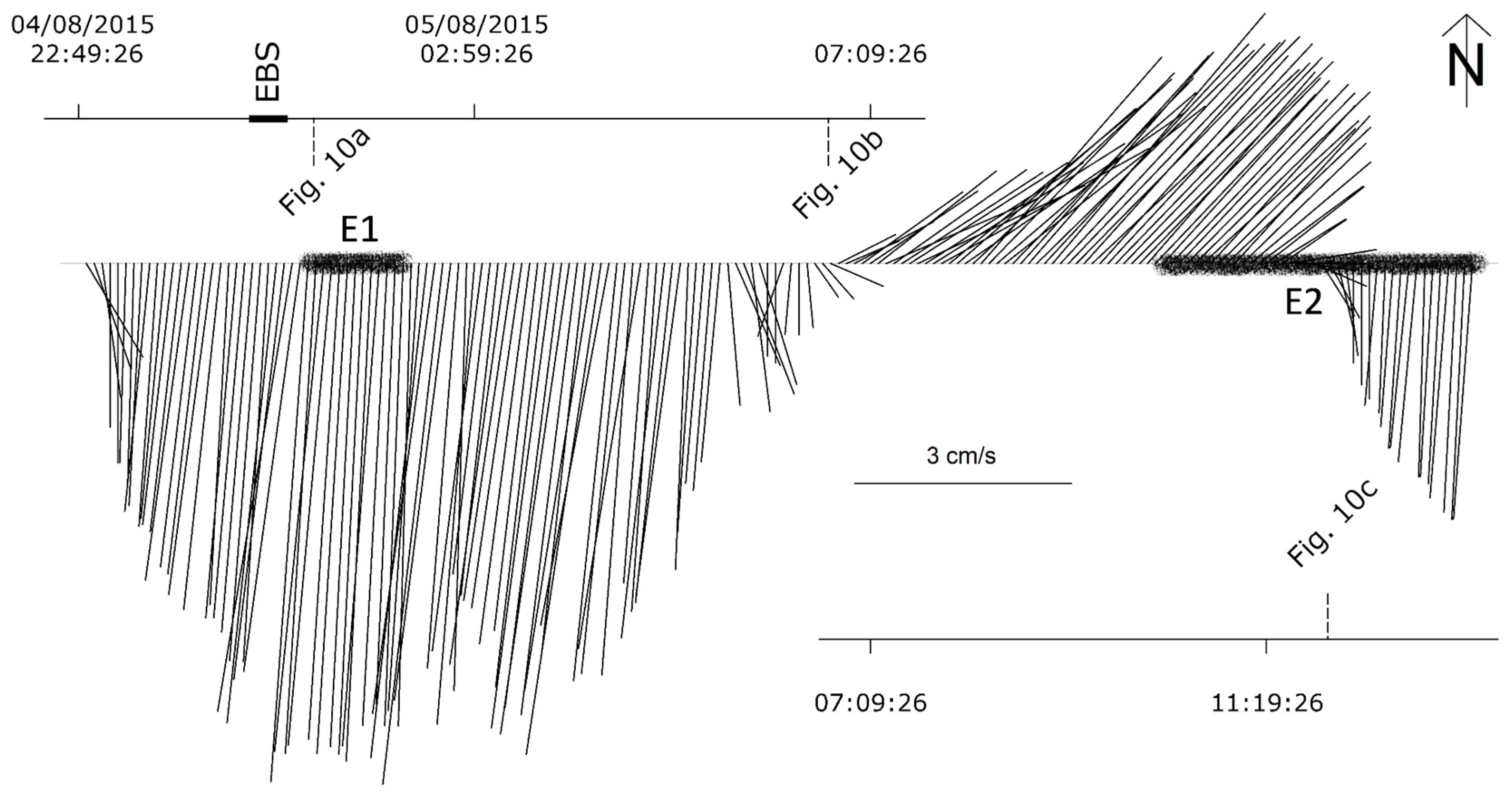
Figure 10.
Figure 10.
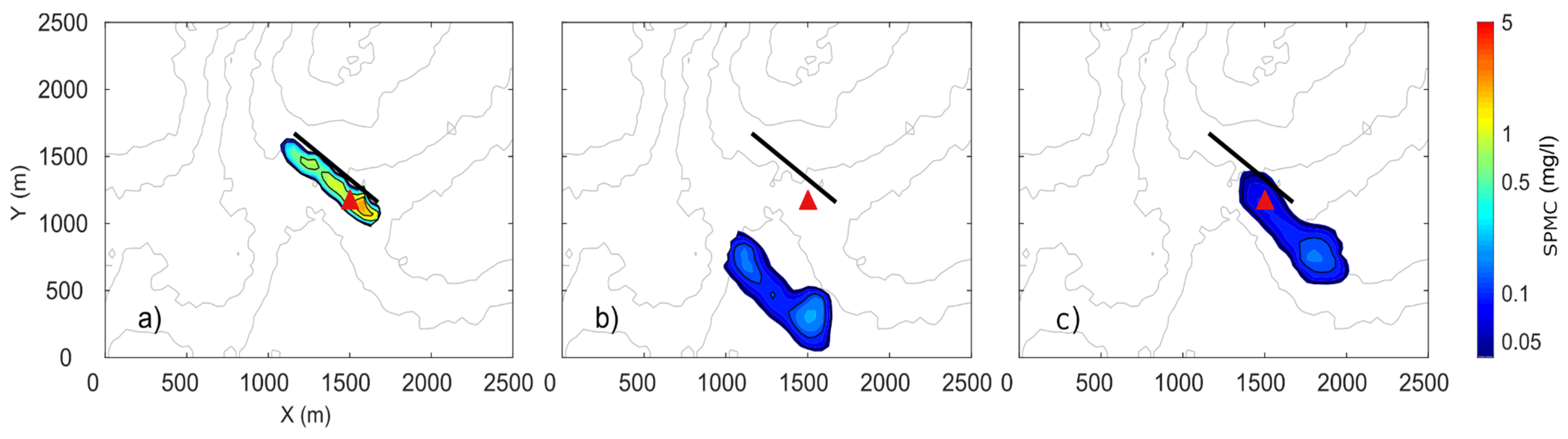
The lateral extension and SPMC of 2 µm class particles in the simulated plume at 0–1 mab (first vertical grid cell). The plume is dispersed and advected by the prevailing current (see
Figure 9). Results are shown 10 min (
a), 6 h (
b), and 11 h (
c) after the end of EBS towing. Black line represents the 740 m long EBS (seafloor erosion) track. Red triangle is the BoBo lander location. The colourbar starts from 0.05 mg/L (near background SPMC).
Figure 10.
The lateral extension and SPMC of 2 µm class particles in the simulated plume at 0–1 mab (first vertical grid cell). The plume is dispersed and advected by the prevailing current (see
Figure 9). Results are shown 10 min (
a), 6 h (
b), and 11 h (
c) after the end of EBS towing. Black line represents the 740 m long EBS (seafloor erosion) track. Red triangle is the BoBo lander location. The colourbar starts from 0.05 mg/L (near background SPMC).
Table 1.
Overview of lander deployments and EBS disturbance test during SO242.
Table 1.
Overview of lander deployments and EBS disturbance test during SO242.
| Stations | Deployment | Recovery | Latitude | Longitude | Water Depth (m) |
|---|
| #11_BoBo-lander-1 | 30 July 2015 18:37 | 05 August 2015 15:20 | −7; 7.465 | −88; 26.086 | 4175 |
| #57_BoBo-lander-2 | 06 August 2015 17:35 | 16 August 2015 06:50 | −7; 04.750 | −88; 28.527 | 4131 |
| #97_BoBo-lander-3 | 16 August 2015 07:43 | 27 August 2015 00:36 | −7; 07.422 | −88; 25.538 | 4162 |
| #6_DOS-lander-1 | 30 July 2015 16:40 | 03 August 2015 04:13 | −7; 04.308 | −88; 28.297 | 4123.6 |
| #42_DOS-lander-2 | 04 August 2015 01:21 | 11 August 2015 14:50 | −7; 04.476 | −88; 26.000 | 4199.2 |
| #72_DOS-lander-3 | 11 August 2015 18:30 | 16 August 2015 09:51 | −7; 04.583 | −88; 28.554 | 4116 |
| #37_EBS-1 | 03 August 2015 08:02 | | −7; 07.686 | −88; 25.706 | 4167.3 |
| | 03 August 2015 09:24 | −7; 07.854 | −88; 25.484 | 4176.3 |
| #45_EBS-2 | 04 August 2015 23:40 | | −7; 07.150 | −88; 26.322 | 4195 |
| | 05 August 2015 00:59 | −7; 07.532 | −88; 25.984 | 4169.7 |
| #34_MUC-6 | 02 August 2015 21:27 | | −7; 07.524 | −88; 27.031 | 4161.7 |
| #70_MUC-17 | 11 August 2015 12:43 | | −7; 04.400 | −88; 27.778 | 4127.5 |
| #119_MUC-31 | 20 August 2015 08:37 | | −7; 06.033 | −88; 24.826 | 4204.1 |
Table 2.
Particle size distribution metrics for the surface sediment layer of the selected 6 multicores. Values between brackets represent pre-treated samples, from which flocculi, carbonates and Fe-Mn oxides have been removed.
Table 2.
Particle size distribution metrics for the surface sediment layer of the selected 6 multicores. Values between brackets represent pre-treated samples, from which flocculi, carbonates and Fe-Mn oxides have been removed.
| | Distribution Parameters | Distribution Percentiles |
|---|
| | Mean | “Stdev” | “Skewness” | “Kurtosis” | 10% | 50% | 90% |
|---|
| 119_MUC-31: 0–5 cm | 24.6 | 40.8 | 3.24 | 12.08 | 1.58
(0.59) | 9.1
(4.24) | 63.3
(37.3) |
| (prep) | (13.9) | (26.83) | (4.45) | (26.58) |
| 119_MUC-31: 5–15 cm | 26.1 | 36.63 | 3.12 | 12.31 | 2.05
(0.68) | 12.9
(4.89) | 62.8
(43.7) |
| (prep) | (16.6) | (31.86) | (4.06) | (20.67) |
| 70_MUC-17: 0–5 cm | 43.3 | 59.18 | 2.53 | 7.16 | 2.88
(0.7) | 21.2
(5.81) | 93.4
(53.2) |
| (prep) | (18.7) | (30.12) | (2.95) | (10.79) |
| 70_MUC-17: 5–15 cm | 23.3 | 30.31 | 3.46 | 17.57 | 1.96
(0.77) | 13.3
(5.95) | 53.9
(48.6) |
| (prep) | (18.4) | (32.41) | (3.76) | (18.11) |
| 34_MUC-6: 0–5 cm | 18.8 | 25.96 | 4.15 | 25.7 | 1.65
(0.78) | 10.4
(6.57) | 61.2
(43,3) |
| (prep) | (22.2) | (37.46) | (3.21) | (12.74) |
| 34_MUC-6: 5–15 cm | 43.3 | 52.71 | 2.14 | 5.13 | 3.1
(0.87) | 23.5
(6.51) | 92.7
(51.6) |
| (prep) | (18.4) | (28.23) | (2.85) | (10.02) |
| Publisher’s Note: MDPI stays neutral with regard to jurisdictional claims in published maps and institutional affiliations. |
© 2021 by the authors. Licensee MDPI, Basel, Switzerland. This article is an open access article distributed under the terms and conditions of the Creative Commons Attribution (CC BY) license (https://creativecommons.org/licenses/by/4.0/).


