Spatial and Temporal Variation in Deep-Sea Meiofauna at the LTER Observatory HAUSGARTEN in the Fram Strait (Arctic Ocean)


1
Alfred-Wegener-Institut Helmholtz-Zentrum für Polar- und Meeresforschung, Am Handelshafen 12, 27570 Bremerhaven, Germany
2
Institute of Oceanology PAS, Marine Ecology Department, Powstancow Warszawy 55, 81-712 Sopot, Poland
*
Author to whom correspondence should be addressed.
Diversity 2020, 12(7), 279; https://doi.org/10.3390/d12070279
Submission received: 7 May 2020
/
Revised: 10 July 2020
/
Accepted: 10 July 2020
/
Published: 13 July 2020
(This article belongs to the Section Marine Diversity)
Abstract
:Time-series studies at the LTER (Long-Term Ecological Research) observatory HAUSGARTEN have yielded the world’s longest time-series on deep-sea meiofauna and thus provide a decent basis to investigate the variability in deep-sea meiobenthic communities at different spatial and temporal scales. The main objective of the present study was to investigate whether the sediment-dwelling meiofauna (size range: 32–1000 µm) is controlled by small-scale local environmental conditions, rather than large-scale differences between water depths. Univariate and multivariate statistical analyses, including distance-based linear models (DistLM) and redundancy analysis (dbRDA), revealed that due to their small size, meiofauna tend to mainly respond to micro-scale (centimeter) variations in environmental conditions in surface and subsurface sediment layers. Inter-annual temporal patterns among metazoan meiofauna at higher taxon levels revealed only a weak effect of time, and merely on the rare meiofauna taxa (<2% of the total meiofauna community) at HAUSGARTEN.
Keywords:
meiofauna; deep-sea; temporal; spatial; time-series; Long-Term Ecological Research; LTER; HAUSGARTEN1. Introduction
The sediment-inhabiting meiofauna is a major component of benthic ecosystems, particularly in the deep sea. Meiofauna organisms are highly abundant, play an important role in benthic food webs, and are vital contributors to ecosystem function [1]. Meiofauna activities modify a series of physical, chemical, and biological sediment properties thereby affecting various ecosystem services, including sediment stabilization, biochemical cycling, waste removal, and food web dynamics [2,3,4,5,6].
Meiofauna abundance, diversity, and community structure commonly vary in time and at all spatial scales, with spatial and temporal variability being generally interactive. At the regional scale, variations in meiofaunal communities appear to be related to differences in surface productivity and the settling of organic matter, representing the major food/energy source for benthic organisms [7,8,9,10]. Bathymetric gradients in meiobenthic community attributes thereby reflect the progressive degradation of organic material on its way to the seafloor. Food and oxygen availability, sediment characteristics, seafloor topography, habitat heterogeneity, and bioturbation by larger fauna typically influence meiobenthic communities at small horizontal and vertical scales [11,12,13,14]. However, generalizations concerning relationships between meiofauna communities and environmental conditions are only difficult to make due to the limited number of studies that allow direct comparisons across multiple scales, including temporal dimensions [10].
In 1999, the Alfred-Wegener-Institut Helmholtz-Zentrum für Polar- und Meeresforschung (AWI) established the LTER (Long-Term Ecological Research) observatory HAUSGARTEN in the Fram Strait between Greenland and Svalbard [15] to detect and track the impact of large-scale environmental changes on the marine ecosystem in the transition zone between the northern North Atlantic and the central Arctic Ocean. Multidisciplinary investigations cover all parts of the open-ocean ecosystem from sea surface to the deep seafloor. Time-series studies at the HAUSGARTEN observatory provide insights into processes and their dynamics within an arctic marine ecosystem, contribute to the global community’s efforts to understand variations in ecosystem structure and functioning on various scales in an overall warming Arctic, and will ultimately allow for improved predictions under different climate scenarios.
Benthic investigations at HAUSGARTEN include spatial and temporal studies of all organism size classes, ranging from bacteria [16,17] to epi/megafauna [18,19,20,21]. Meiobenthic studies focused on the metazoan community, excluding foraminiferans [22,23]. The present study focuses on results from 15 years of continuous sampling at a comparably shallower site at ~1280 m, an intermediate site at ~2500 m, and a deep-water site at ~4000 m water depth on the continental margin off Svalbard between 2000 and 2014.
Data from these investigations provide a decent basis to investigate the spatial and temporal variability in deep-sea meiobenthic communities. The main objective of the present study is to investigate whether the sediment-dwelling meiofauna is controlled by small-scale local environmental conditions, rather than large-scale differences between water depths, by addressing the following questions: (1) Do deep-sea meiofauna communities vary in abundance and structure at temporal and different spatial scales? (2) Are deep-sea meiofauna communities correlated with environmental variables at temporal and different spatial scales? (3) Do different spatial scales contribute differently to the overall variability of the community structure? (4) Are the effects of temporal changes in environmental variables on meiofauna communities comparable to the effects of spatial changes in environmental variables?
2. Materials and Methods
2.1. Study Site
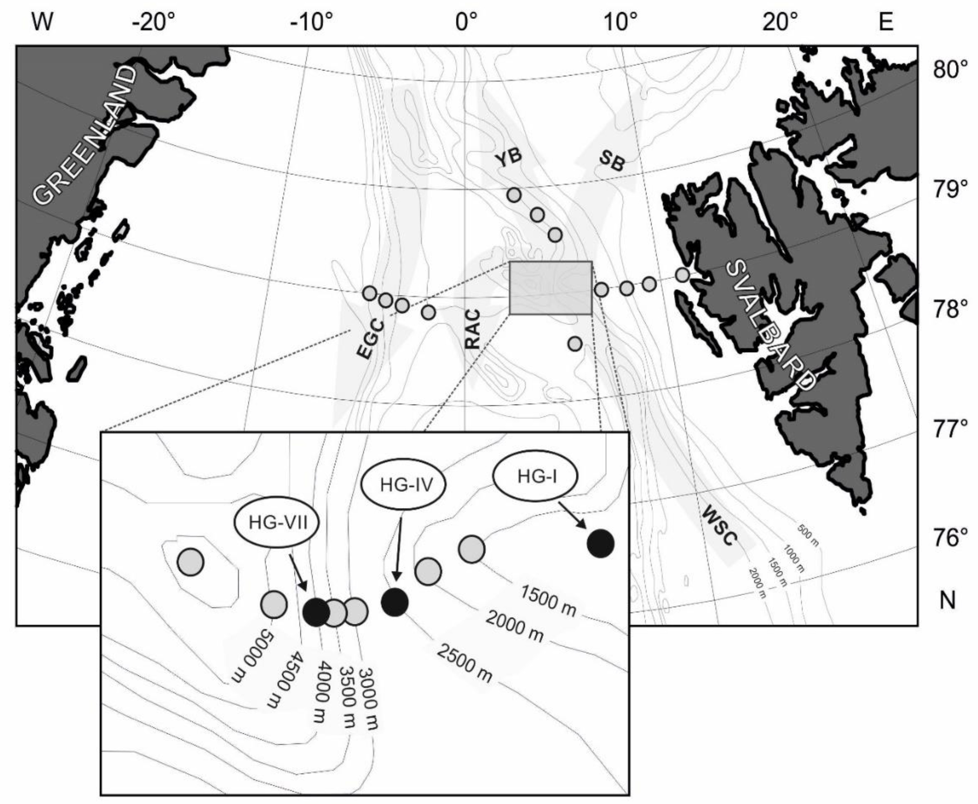
Time-series studies were carried out at the LTER observatory HAUSGARTEN in the Fram Strait (Figure 1). The observatory comprises a network of 21 sites along two transects: a latitudinal isobathic transect at approximately 2500 m water depth between 78°30′ N and 80°00′ N in the eastern Fram Strait between 3° E and 5° E, and a longitudinal bathymetric transect with site depths ranging between 250 m and 5500 m water depth between 5°00′ W and 11°00′ E, crossing the strait at about 79° N (for a more detailed site description see [24]).
The Fram Strait is the only deep-water connection between the Nordic Seas and the central Arctic Ocean with a sill depth of approximately 2600 m. The hydrography in the eastern part of the strait is characterized by the inflow of relatively warm and nutrient-rich Atlantic Water (AW) into the central Arctic Ocean [25]. Cooler and less-saline Polar Water exits the central Arctic Ocean as the Eastern Greenland Current (EGC) in the western part of the Fram Strait [26], separated by a frontal system (East Greenland Polar Front) from the water masses in the eastern part of the Fram Strait [27]. Hydrographic patterns in the strait result in a variable sea-ice cover, with predominantly ice-covered areas in the west, permanently ice-free areas in the south-east, and seasonally varying ice conditions in the central and north-eastern parts.
Meiofauna investigations for this study were restricted to a subset of sites along the bathymetric transect in eastern parts of the strait, with a total of three permanent sampling sites at approximately 1280 m (HG-I), 2500 m (HG-IV), and 4000 m water depth (HG-VII) off Svalbard. Distances in nautical miles (nm) between sites were about 7.5 nm between HG-VII and HG-IV, and 22.5 nm between HG-IV and HG-I; the distance between HG-I and the Svalbard coast is approximately 58.5 nm (Figure 1).
2.2. Annual Sediment Sampling
During the annual summer cruises to Fram Strait, a multiple corer (MUC) was used to retrieve surface sediments at all HAUSGARTEN sites. Table 1 provides an overview of the stations selected to study spatial and temporal variations in meiofauna communities between 2000 and 2014 (15 years). Due to logistical constraints, samples from the deepest site HG-VII were missing for the 2009, 2013, and 2014. Subsamples to evaluate individual abiotic and biotic parameters (see below) were taken from the MUC tubes (10 cm in diameter and 50 cm in length) by means of plastic syringes with cut-off anterior ends (1 and 2 cm in diameter and 5 cm in length). Sediment cores were sectioned in 1-cm layers to study vertical gradients of all parameters in the uppermost 5 cm of the sediments.
2.3. Sample Processing for Meiofauna Organisms
Three subsamples (2 cm in diameter and 5 cm in length) from different MUC tubes were taken for meiofaunal studies. Organisms that pass through a 1-mm sieve were enumerated under a low-power stereo microscope after washing the Rose Bengal stained sediment samples through a set of sieves with various mesh sizes (500, 250, 125, 63, and 32 µm) to facilitate further processing (cf. [28]). Meiofaunal organisms were identified to major taxa, i.e., Nematoda, Copepoda (including nauplii), Ostracoda, Kinorhyncha, Polychaeta, Tardigrada, Gastrotricha, and Platyhelminthes. All taxa occurring in low abundance (e.g., Loricifera, Acari, Oligochaeta, Sipunculida, Tanaidacea) were pooled as ‘Others’. Meiofauna densities were standardized to individuals per 10 cm2.
2.4. Assessment of Environmental Background Data
Environmental parameters measured in this study include abiotic sediment characteristics and different biogenic sediment compounds indicating food/energy input to the seafloor as well as the organic matter content and the microbial biomass in the sediments from the selected sites. Each time three sediment cores of 2 cm in diameter and 5 cm in length were taken to determine grain size spectra as well as water and total organic matter contents; sediment cores to analyze organic carbon contents and chloroplastic pigments were 1 cm in diameter and 5 cm in length.
Grain size analyses were performed by wet sieving [29]. Considering the overall very low sedimentation rates (usually below 1 mm per century; [30]) and low bioturbation rates at the deep seafloor in Fram Strait [31], it could be assumed that the sediment composition and stratification will not significantly change over a course of 15 years. Grain size analyses were therefore only conducted once on samples taken during an expedition to HAUSGARTEN in summer 2015.
Water contents (H2O), indicating the porosity of the sediments, were determined by measuring the weight loss of wet sediment samples dried at 60 °C. Total organic matter contents were determined as ash-free dry weights (AFDW) after combustion of the dried sediments (2 h at 500 °C [32]. The availability of phytodetritial matter, which represents the prime food source for benthic organisms, was assessed by measurements of sediment-bound chlorophyll a and its degradation products (phaeopigments). Chloroplastic pigments were extracted in 90% acetone and measured with a Turner fluorometer [33]. The bulk of pigments (chlorophyll a (CHLA) plus their degradation products, i.e., phaeopigments (PHAEO)) registered by this method was termed chloroplastic pigment equivalents, CPE [34]. The “freshness” of the phytoplankton-derived particulate organic matter at the seafloor was estimated by the proportion of chlorophyll a (%CHLA) from the total pigment content (CPE). Phospholipid concentrations (LIPIDS) were determined to estimate the total microbial biomass in the sediments [35].
2.5. Statistical Analyses
Differences in total meiofauna densities between water depths and between years were separately tested for each site (HG-I, HG-IV, HG-VII) using rank-based non-parametric (Kruskal–Wallis) one-way analysis of variance. Post-hoc tests for multiple comparisons between years were performed. For each pairwise comparison, p-values (bilateral significance level) were calculated with the Bonferroni correction. All univariate statistical analyses were performed with the STATISTICA 10 software (StatSoft, 1984–2011). Linear regression to model the relationship between meiofaunal densities and time (2000–2014) by fitting a linear equitation to the observed data was done using the regression option implemented in the Data Analysis add-in of MS Excel (2016).
Patterns in community composition and structure were described using the hierarchical cluster analysis in PRIMER [36]. Similarity matrices were built using Bray-Curtis similarity of square-root transformed abundance data; all samples from all years (2000–2014) and all sites (HG-I, HG-IV, HG-VII; including generally three [pseudo]replicates per site and sampling date) were included in the analyses. A similarity profile test (SIMPROF) was performed to identify natural group structure in the samples [37]. The SIMPROF routine conducts a series of permutation tests to find clusters of samples with statistically significant internal structure (p set at 0.05; [36]). Results of the SIMPROF routine were superimposed as factor on a non-metric multi-dimensional scaling (MDS) plot. The SIMPER routine in PRIMER was used to identify the taxa contributing most to within-group similarity and between-group dissimilarity [36].
Relationships between environmental, spatial, and temporal parameters as well as meiofauna community structure were analyzed using distance-based linear models (DistLM) [38]. The resemblance matrix (Bray-Curtis similarity) of meiofauna community data was based on square-root transformed abundance data of the meiofaunal taxa. The predicting environmental variables allowed to enter the distanced-based model were H2O, AFDW, CHLA, and LIPIDS (data for these parameters are available for each year and at each sampled site; PHAEO, CPE, and %CHLA were not included in the analysis with regard to autocorrelations between the variables; median grain sizes were excluded, because values were assessed only once for the three sites). After assessing normality and collinearity of the other predictor variables using a draftsman plot, CHLA data was transformed using the natural logarithm to correct for skewness [39]. No pair of variables was correlated by R > 0.85 and hence all variables were retained for possible inclusion in the model. Predicting spatial variables were water depth (WATER-DEPTH) and sediment depth (SED-DEPTH), predicting temporal variable was sampling year (YEAR).
Initially, the relationship between predictive variables and meiofauna communities were examined by analyzing each of the predictors (i.e., year, sediment depth, water depth, food availability and sediment characteristics) separately (marginal tests). The relationship between meiofaunal community structure and the environmental parameters (sediment characteristics and food availability) was examined given the effect of the spatial variables by entering sediment depth and water depth as starting terms [39]. The specified selection procedure was applied for the environmental parameters using adjusted (R2adj) as a selection criterion to consider the different number of variables within each parameter [39].
To determine the proportion of total variation explained by the each predictor parameter to the overall model, the variability in meiofauna abundance taxa was partitioned into: (1) ‘pure’ environmental variation, or the proportion of variation explained by environmental parameters independently of spatial and temporal parameters; (2) ‘pure’ spatial variation, or the proportion of variation explained by spatial parameters independently of environmental and temporal parameters; (3) ‘pure’ temporal variation, or the proportion of variation explained by temporal parameters independently of environmental and spatial parameters; (4) spatio-temporal structured environmental variation, or the proportion of variation explained by the combination of environmental, spatial and temporal parameters; and (5) unexplained variation, or the fraction of variation not explained by either environmental, spatial, or temporal parameters in the DistLM models (for details see [40,41]).
We then investigated the relationship between spatial parameters and meiofauna community given the effect of temporal parameters by using the same approach (i.e., by entering years as starting terms, followed by all specified selection procedure for the spatial parameters using R2adj as selection criterion). The same approach was applied to examine the relationship between temporal parameters and meiofauna community structure given the effect of environmental variables by entering sediment characteristics and food availability as starting term. The p-values for individual predictor variables were obtained using 9999 permutations of raw data [39]. We used the same approach (all specified selection procedure with adjusted R2 selection criterion) to examine the relationship between environmental predictors and meiofauna community patterns (Bray-Curtis similarity matrix based on fourth-root transformed abundance data) and visualized the results with a distance-based redundancy analysis (dbRDA) [39].
All multivariate statistical analyses were performed using the PRIMER 7 (v. 7.0.13.) statistical package with the PERMANOVA+ add-on (PRIMER-E, Plymouth Marine Laboratory, Plymouth, UK).
3. Results
3.1. Meiofaunal Data
Meiofauna densities (mean values over 15 years) showed significant differences (Kruskal-Wallis H(2,n = 855) = 75.4725, p = 0.00001) between the three water depth layers, with 2278 ± 764 ind. 10 cm−2 at 1280 m water depth (range: 665–3298 ind. 10 cm−2), 1216 ± 649 ind. 10 cm−2 at 2500 m (range: 496–2965 ind. 10 cm−2), and 406 ± 198 ind. 10 cm−2 at 4000 m (range: 148–808 ind. 10 cm−2) (Table 2).
Figure 2 illustrates the temporal patterns of meiofauna densities at the three water depth layers between 2000 and 2014. Especially the shallower and the intermediate site (HG-I, HG-IV) showed conspicuous inter-annual variability in meiofauna densities, compared to the deeper site (HG-VII). Also, small-scale variability between the three (pseudo)replicates per site was clearly higher at HG-I and HG-IV, compared to HG-VII.
Intriguingly, the temporal patterns in meiofauna numbers showed no synchronicity between the different water depth layers (Figure 2). At the shallowest site (HG-I), meiofaunal densities showed a significant drop (Kruskal-Wallis, p = 0.0069; Table 3) between 2009 (664 ind. 10 cm−2) and 2011 (2779 ind. 10 cm−2), afterwards continuously rising again, but (until 2014) not reaching abundance levels before 2009 (Table 2). At the intermediate site (HG-IV), densities displayed a conspicuous (non-significant) decline between 2002 (2055 ind. 10 cm−2) and 2005 (818 ind. 10 cm−2) as well as a highly significant decrease between 2007 (2965 ind. 10 cm−2) and 2010 (496 ind. 10 cm−2; Kruskal-Wallis, p = 0.0001; Table 3). At the deepest site (HG-VII), meiofauna densities showed a (non-significant) decrease between 2001 (808 ind. 10 cm−2) and 2004 (148 ind. 10 cm−2). However, over the entire period, values stayed approximately at a similar level at this site. Considering the meiofauna densities over the entire 15 years (2000–2014) of observations, an overall (non-significant) decrease becomes obvious, most pronounced at the shallowest site (HG-I) (Figure 2).
Nematodes generally dominated the metazoan meiofauna (mean for all sites and years: 95.2 ± 2.8%), copepods were second dominant (mean for all sites and years: 3.1 ± 2.1%), while all other meiofauna taxa occurred only in very minor quantities (mean for the sum of all other taxa: 1.7 ± 1.6%). Neglecting the constantly high dominance of nematodes at all sites and in all sampling years, the percentages of other meiofauna taxa showed a conspicuous trend with decreasing proportions of copepods in relation to the percentage of all other meiofauna taxa with increasing water depth (data not shown).
The temporal variation in meiofauna taxa occurring in very minor numbers (<2%) generally followed total meiofauna densities (Figure 3). However, although total meiofauna numbers showed again increasing values in the years 2011 till 2014 (especially at the shallowest site HG-I), meiofauna taxa generally occurring at minor quantities stayed at a comparably low level. Unfortunately, data for the deepest site HG-VII are partly missing to confirm that this trend holds for all site depths.
Cluster analyses based on meiofauna abundance in the different sediment layers (0–5 cm) at HG-I, HG-IV, and HG-VII between 2000 and 2014 revealed a total of ten significant SIMPROF groups (SFG), which can be categorized into six broader groups (i.e., a, b and c, d, f, h and i, j). SFGs are visualized as factors in an MDS plot (Figure 4). Meiofauna communities within SIMPROF-groups are spatially characterized, the temporal aspect was not important. The communities are mainly grouped according to their occurrence within certain sediment layers at the different sites (i.e., water depths). The groups g and e are composed of only two samples each (taken at different sites in different years) and clustered because they are characterized by the fact that, apart from nematodes, no other taxa were represented (except for one sample, in which a single kinorhynch was recorded).
SIMPER analyses revealed that nematodes (as the only taxon for most groups) are responsible for the similarities within each of the ten groups. Dissimilarities between groups are mainly based on nematodes together with copepods (including nauplii). An exception were the differences between groups g and e and all other groups, where mainly the rare meiofauna taxa (e.g., Ostracoda, Bivalvia, Kinorhyncha, Tardigrada) are responsible for the differences between groups g and e and the remaining groups.
3.2. Environmental Data
Median grain sizes (Table 4) were lowest at the shallowest site HG-I (8.13 ± 3.79 µm; mean values for the uppermost 5 cm of the sediments) and continuously increased towards the deeper sites (21.32 ± 2.43 µm at HG-IV and 37.26 ± 5.97 µm at HG-VII; mean values for the uppermost 5 cm of the sediments).
Except for phospholipid concentrations in the sediments, all other environmental parameters showed generally decreasing values with increasing water depth (Table 5). Mean water content at the shallowest site (HG-I) was 64.8 ± 3.6%, 50.7 ± 1.4% at intermediate depth (HG-IV), and 37.1 ± 4.5% at the deepest site (HG-VII). Total organic matter decreased from 114.7 ± 24.5 µg cm−3 at HG-I to 107.6 ± 18.6 µg cm−3 at HG-IV, and 92.6 ± 18.0 µg cm−3 at HG-VII. The proportion of organic carbon had almost halved from 1.3 ± 0.2% to 0.7 ± 0.1% between the shallowest and the intermediate site (HG-I and HG-IV, respectively) but showed a similar value at the deepest site (HG-VII). The total pigment content of the sediments steeply decreased from 20.5 ± 10.0 µg cm−3 at HG-I to 9.9 ± 3.8 µg cm−3 at HG-IV and 5.6 ± 3.3 µg cm−3 at HG-VII. The proportion of chlorophyll a, indicating the quality of the phytodetritial matter reaching the seafloor, followed the same trend with decreasing values with increasing water depth (average values: 13.9 ± 5.2% at HG-I, 11.0 ± 3.6% at HG-IV, and 9.0 ± 5.7% at HG-VII). Phospholipid concentrations almost halved from 15.3 ± 8.4 mmol cm−3 to 8.5 ± 4.2 mmol cm−3 between the shallowest and the intermediate sites but increased again to 10.3 ± 5.1 mmol cm−3 at the deepest site.
The temporal patterns in the environmental data at the selected HAUSGARTEN sites between 2000 and 2014 revealed diverse patterns (Figure 5). The inter-annual variability of specific parameters, i.e., water content and total organic matter, showed only minor variation in time, while other parameters, i.e., chlorophyll a and phospholipids, exhibited increased variability between the years, partly in parallel to each other, and in parts also between the different water depth horizons.
3.3. Relationships between Meiofaunal and Environmental Data
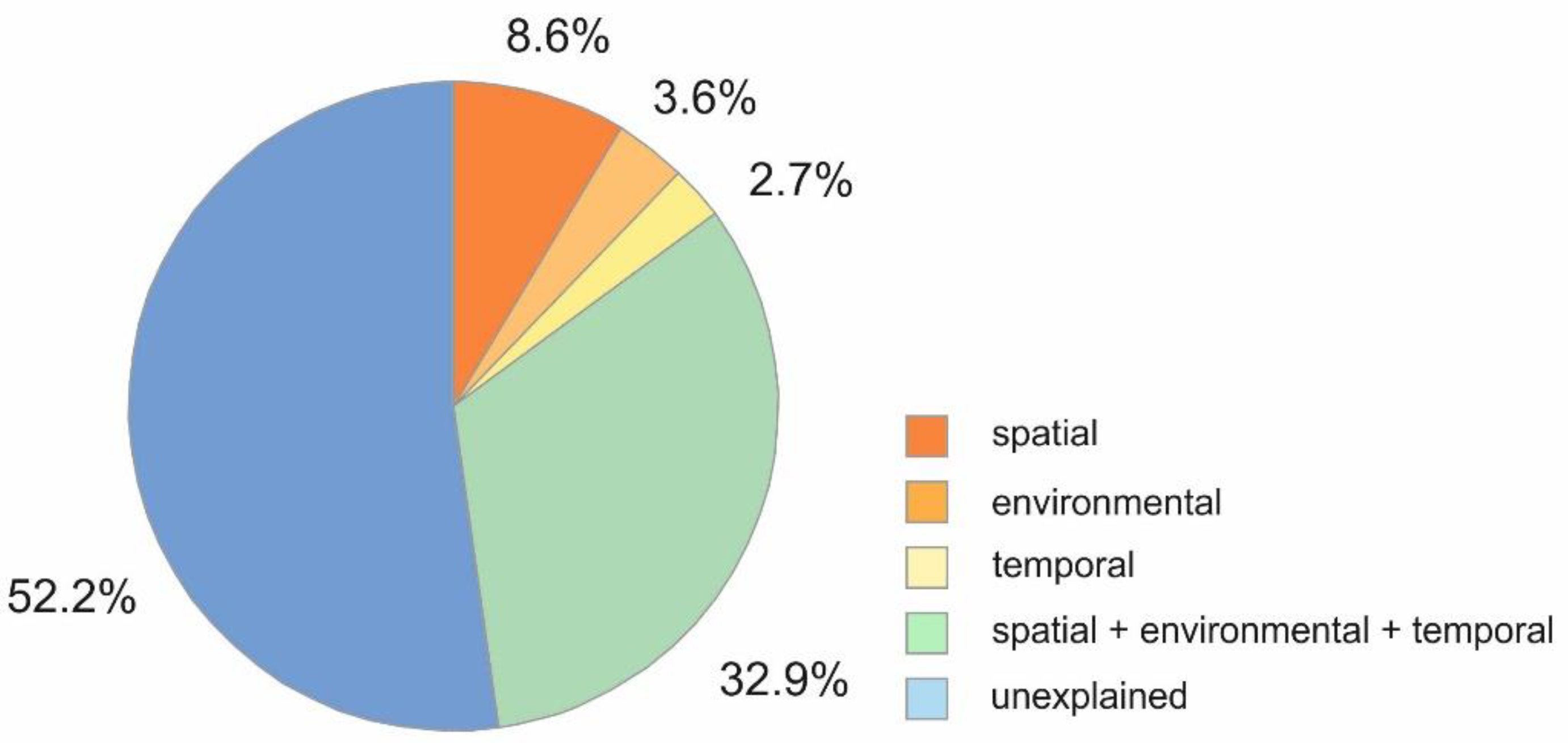
Variation in meiofauna abundance in DistLM models combining all explanatory variables was partitioned in environmental (parameters indicating food availability and sediment characteristics), spatial (water depth, sediment depth) and temporal (sampling year) variables. All tested variables together explained 47.8% of meiofauna variation, while 52.2% of the total variation cannot be explained by the tested variables. Environmental variation alone accounted for 3.6%, spatial variation for 8.6%, temporal variation for 2.7%, and spatio-temporal structured environmental variation for 32.9% of the explainable variability (Figure 6).
Results from DistLM analyses on the relationship between environmental, spatial, and temporal parameters on meiofauna community structure (Table 6) revealed that all parameters, apart from total organic matter content of the sediments, were significantly correlated with meiofaunal community structure in marginal tests (p < 0.05). The strongest relationships were found for sediment porosity (31%) as well as spatial related parameters (sediment depth = 22%, and water depth = 19%) together with aspects of food availability (chlorophyll a: 15%), which explained significant amounts of variation (p < 0.01). Phospholipid concentrations and the temporal structure of the data explained only small amounts of variation (5% and 2%, respectively), but were nevertheless found to be statistically significant (p < 0.01 and p ≤ 0.05, respectively).
In sequential tests, when fitting environmental parameters first, >35% of the variation is explained (p < 0.01); spatial and temporal parameters added comparably small proportions to the explained variation (9.6% and 2.7%, respectively), thereby still being highly significant (p < 0.01) (Table 6). With spatial parameters as a starting term, 42% of variation is explained, while temporal and environmental parameters account for only 2.3% and 3.6%, respectively, of the overall explained variation (Table 6); nonetheless, all parameters were still highly significant. When fitting temporal parameters first, followed by environmental and spatial parameters, we found environmental parameters explained the largest proportion of variation (37.6%), even after fitting temporal parameters (Table 6). Temporal parameters accounted for the smallest proportion of the explained variation and were no longer highly significant (p < 0.05). The weak relationship between temporal parameters and meiofauna community is also expressed by the low R2 values in all combined models (0.01–0.03), whereas environmental and spatial parameters showed the highest R2 values of 0.37, when fitting temporal parameters first, and spatial R2 values of 0.41, when fitting spatial parameters first.
When performing the same DistLM analyses (separately for each site) with a similarity matrix based on meiofaunal densities exclusively for the rare taxa (excluding nematodes and copepods), marginal tests showed a much stronger relationship between time (Year) and meiofauna communities. Apart from water depth and sediment depth, the temporal parameter explained the largest proportion of meiofaunal variation at sites HG-I (9.8%, p = 0.001) and HG-VII (14.2%, p = 0.001). At HG-IV, environmental parameters (chlorophyll a = 5.4%, total organic matter = 7.2%, and water content = 7.7%) still explain the larger proportions of variation compared to time (Year = 3.2%, p = 0.014).
The full DistLM was visualized by examining the dbRDA ordination (Figure 7). The first two dbRDA axes captured nearly 97% of the variability in the fitted model, which is about 53% of the total variation in the meiofauna data cloud. The vector overlay shows that the first dbRDA axis is particularly strongly related to porosity (H2O), sediment depth (SED-DEPTH), and water depth (WATER-DEPTH). The temporal effect (YEAR) and parameters indicating food availability (AFDW, CHLA, LIPIDS) are related to the second dbRDA axis. H2O showed the strongest relation to dbRDA1 followed by SED-DEPTH at the spatial level. WATER-DEPTH, also related to dbRDA1, contributed less to variation along dbRDA1, whereas food availability in terms of CHLA showed by far the strongest relation to dbRDA2. The temporal effect (YEAR) also contributed to variation along dbRDA2.
4. Discussion
To our knowledge, long-term ecological studies at the HAUSGARTEN observatory, with data collected annually in the summer months since 2000, have yielded the world’s longest time-series on deep-sea meiofauna [42,43,44]. Data from these long-term investigations provide a decent basis to study the variability in deep-sea meiobenthic communities at different spatial and temporal scales.
4.1. Spatial and Temporal Patterns in Deep-Sea Meiofauna Communities at HAUSGARTEN
Meiofauna densities in the eastern Fram Strait at different water depths off Svalbard (1280 m, 2500 m, and 4000 m) decreased with increasing water depth and could validly be explained by the gradually decreasing food/energy availability at the seafloor. At the same time, meiofauna numbers showed substantial inter-annual variability but also conspicuously and, in part, substantially oscillating values (Figure 2). At the shallowest site (HG-I) investigated in this study, the temporal patterns in meiofauna numbers showed a strong relationship with the quality of phytodetritial matter at the seafloor (indicated by the proportion of chlorophyll a from the total pigment content of the sediments), while at deeper sites (HG-IV and HG-VII) this relationship almost vanished. These findings might suggest that the quality rather than the quantity of phytodetritial matter may play a stronger role at shallower water depths, compared to deeper depths. However, it must be considered that we tried to establish relationships between environmental variables and meiofauna organisms at higher taxonomic level, while species within each higher taxonomic group are characterized by different physiological characteristics, feeding preferences, life cycles, and reproduction rates. As a result, they might react individually to changes in parameters such as the quantity and quality of available food [45]. In addition, predation by larger benthic organisms might considerably affect relationships that may exist between meiofaunal organisms and environmental parameters, especially at the shallowest site HG-I, where macrofauna densities are twice as high and megafauna densities are almost 3-times higher compared to the intermediate site HG-IV [18,46], while their densities at the deepest site HG-VII were comparable to those found at intermediate depths.
Still, despite the inter-annual variability in meiofauna densities at all sites investigated on the continental margin off Svalbard, 15 years of continuous sampling exhibited an overall trend with generally declining meiofauna numbers, most pronounced at the shallowest depth (1280 m) and with decreasing strength at deeper sites (Figure 2). This overall trend occurs most prominently in the group of meiofauna taxa generally occurring at minor quantities (<2%) (Figure 3). Although sediment-bound pigment concentrations generally increased in the same time period, an apparently decreasing quality of the phytodetritial matter at the seafloor, as indicated by overall declining values in the proportion of intact chlorophyll a from the total pigment content of the sediments between 2000 and 2014, might explain the overall decrease in meiofauna densities, at least for the shallowest site.
Interestingly, the temporal patterns in meiofauna numbers showed no synchronicity between the different water depth layers, i.e., peaks in meiofauna densities occurred in different periods over the time frame investigated in this study. Although all three sites are located in the same area, it looks as if meiofauna maxima at the shallower sites are preceded by similar maxima on the respective deeper sites by about 1–2 years (Figure 2). A possible explanation for these findings might be that meiofauna communities at greater water depths, inhabiting sediments usually characterized by generally lower organic matter contents and more a variable food availability, are more vulnerable to temporal variations in food/energy availability compared to those communities living in shallower sedimentary environments with higher organic matter contents, i.e., a comparably enriched food reservoir. Results from time-series studies within the FOODBANCS project on the Antarctic shelf [47], suggesting that the accumulation of organic matter in sediments (or generally increased organic matter contents) may buffer the benthic ecosystem from temporal variability of processes in the water column (primary production and the settling of organic matter), might support this hypothesis.
In parts, the temporal patterns in the meiofauna numbers can be related to a warming event in the Atlantic Water layer which was associated with temporarily increased salinities in the eastern Fram Strait between 2005 and 2008 [48]. This anomaly left a strong “footprint” within the arctic marine ecosystem in the HAUSGARTEN area [24]. Impacts of the anomaly encompassed the increased growth of sub-arctic primary producers [49] as well as a northward displacement, increased abundance and reproductive output of sub-arctic pelagic species, leading finally to changes in community structure due to range shifts [50,51,52,53,54]. Cascading effects, propagating through the entire marine food web, led to an astoundingly rapid and far-reaching reaction of the entire open-ocean ecosystem from the pelagic to the deep seafloor. Temporarily increased meiofauna densities at all benthic sites investigated in this study could therefore directly be related to variations in the overlying waters between 2005 and 2008. A second period of increased water temperatures and salinities in 2011/2012 [48] might have had a similar effect on the pelagic system in the eastern Fram Strait. As in 2006, a massive bloom of the haptophyte Phaeocystis pouchetii was also observed in 2012 [49,55]. The settling of this phytoplankton bloom could thus probably also explain the again rising meiofauna numbers in the years 2011 till 2014 (Figure 2).
4.2. Sources of Variation in Deep-Sea Meiofauna Communities at HAUSGARTEN
Our comprehension of the level of meiofauna community structure and the degree of spatial and temporal variability in benthic community composition in the deep sea as well as the responsible drivers is still incomplete. In the present long-term study, we used different environmental and spatial explanatory variables to describe variation in meiofaunal communities over a time period of 15 years.
Statistical analyses revealed that the largest proportion of variation in meiofauna community structure was explained by pure spatial variation (8.6%), followed by environmental parameters (3.6%) (Figure 6). The effect of temporal parameters has the lowest impact on the variability of the community in all models (2.7%) (Figure 6). Nevertheless, a DistLM showed that all parameters are significantly correlated with the variability in community composition. Spatial parameters explained the greatest variability (42%), when considered first. After considering the effect of the environmental parameters, which explain 38% of the variability, 10% of the variability is still explained by the spatial parameters. Much of the spatial variation was accounted for by sediment depth, which explained 22% of the variability in meiofauna community structure in marginal tests (see Table 6). While these results do not provide information about the underlying processes, they are an indication that a considerable proportion of variation is associated with processes at the small scale of sediment depth [10].
At all the sites, meiofaunal densities were highest in the surface sediment layer (0–1 cm) and decreased with increasing sediment depth (down to 4–5 cm). These differences in meiofaunal distribution at the small spatial scale with increasing sediment depth were stronger than those at the larger scale among the three sites, i.e., along the bathymetric gradient (see also [43]). Studies of meiofauna along bathymetric gradients are usually seen as studies at the habitat scale and a recent review of ecological studies on deep-sea meiofauna confirmed that habitat-scale effects on meiofaunal communities are often less pronounced than regional or small-scale effects [10].
At the small, sediment-depth scale, food proxies and sediment characteristics, amongst others, are the typical factors influencing meiofauna communities [10]. Although environmental parameters explained a clearly lower portion (3.6%) in the variability of the meiofauna community structure in the present study (Figure 6), they still have a much greater influence than spatial parameters, after considering the effect of time. In addition, marginal tests showed that parameters best correlated to the vertical patterns in the meiofaunal community structure were the environmental factors water content (porosity) and the availability of “fresh” phytodetrital material (chlorophyll a) (Table 6). Therefore, the heterogeneity of the environment seems to be a descriptor for spatial rather than temporal patterns. In polar regions, the bulk of benthic meiofauna basically feeds on degraded organic matter, a food source available throughout the year [56], and variations in meiofauna abundance and community structure can be explained by the input and availability of organic matter [57,58]. In accordance with the DistLM (Table 6), results visualized by dbRDA (Figure 7) suggest that meiofaunal community structure is mainly influenced by small-scale variability at a centimeter scale. However, compared to small-scale spatial variability, temporal (inter-annual) variation in food availability has a lesser impact on the community composition.
In general, variability in abundances in correlation with environmental heterogeneity inevitably occurs at a hierarchy of spatial and temporal scales (e.g., [59,60]), whereas spatial and temporal variability are generally interactive [61]. The present study in fact revealed that the interaction of all parameters explained a substantial part of variation (32.9%) (Figure 6). Nevertheless, the largest part (52.2%) remained unexplained by the tested parameters, indicating that some unmeasured underlying processes are affecting meiofauna community patterns. The number of groups identified by the hierarchical cluster analyses and SIMPROF depended largely on the vertical distribution patterns of nematodes, the most common meiofauna taxon, which explained most of the similarity within each group. Taking this into account, the weak effect of time on the community patterns might indicate that time hardly influences the dominance of the taxon Nematoda as such.
Finally, results from our statistical analyses have also shown that time has an effect on the rare meiofauna, i.e., taxa that make up <2% of the total meiofauna. This leads to the assumption that time may influence the different meiofauna groups in different ways [45]. Consequently, some meiofaunal responses to inter-annual environmental changes may be masked at the level of higher taxa [45,62].
5. Conclusions
In conclusion, the present results are largely consistent with the generally accepted findings that metazoan meiobenthos densities in the deep sea are much more variable on a small scale than in shallow waters. Due to their small size, meiofauna tend to respond to micro-scale (centimeter) variability of environmental conditions in surface and subsurface sediment layers [63,64,65,66]. Sediment granulometry and differences in geochemical and physical properties on a vertical scale are known to be reflected in meiofaunal community composition [66,67], whereas the distribution of meiofauna in the sediments is mainly controlled by food and oxygen availability in subsurface sediments [66,68,69,70,71]. Inter-annual temporal patterns among metazoan meiofauna at higher taxon levels revealed only a weak effect of time on the deep-sea meiofauna community at the LTER observatory HAUSGARTEN. Although other studies came to similar results [45,72], it can be assumed that more detailed observations at higher taxonomic resolution might have detected any long-term changes that have occurred.
Author Contributions
All authors have equally contributed to the conceptualization of the idea and the methods used. Data acquisition (sampling and samples processing) were coordinated by C.H. and K.G., C.H. had conducted statistical analyses and data interpretation was done by all authors. T.S. prepared the original draft with considerable contributions from C.H. All authors have substantially contributed to the writing of the final text. Moreover. All authors have read and agreed to the published version of the manuscript.
Funding
This research received no external funding.
Acknowledgments
We would like to thank the officers and crews of RVs Polarstern, Maria S. Merian, and L’Atalante for their support during our expeditions to the LTER observatory HAUSGARTEN between 2000 and 2014. Anja Pappert and numerous lab apprentices and student assistants are gratefully acknowledged for their assistance with the measurements of various abiotic and biotic sediment parameters, bacterial counts, and meiofauna sortings. We also gratefully acknowledge three anonymous reviewers for their valuable comments on the manuscript. This is publication “e-51702” of the Alfred-Wegener-Institut Helmholtz-Zentrum für Polar- und Meeresforschung, Bremerhaven, Germany.
Conflicts of Interest
The authors declare no conflict of interest.
References
- Schratzberger, M.; Ingels, J. Meiofauna matters: The roles of meiofauna in benthic ecosystems. J. Exp. Mar. Biol. Ecol. 2017, 502, 12–25. [Google Scholar] [CrossRef]
- Coull, B.C. Are members of the meiofauna food for higher trophic levels? Trans. Am. Microsc. Soc. 1990, 109, 233–246. [Google Scholar] [CrossRef]
- Nehring, S. Tube-dwelling Meiofauna in Marine Sediments. Int. Rev. ges. Hydrobiol. Hydrogr. 1993, 78, 521–534. [Google Scholar] [CrossRef]
- Meysman, F.J.; Middelburg, J.J.; Heip, C.H. Bioturbation: A fresh look at Darwin’s last idea. Trends Ecol. Evol. 2006, 21, 688–695. [Google Scholar] [CrossRef]
- Näslund, J.; Nascimento, F.J.; Gunnarsson, J.S. Meiofauna reduces bacterial mineralization of naphthalene in marine sediment. ISME J. 2010, 4, 1421–1430. [Google Scholar] [CrossRef] [PubMed]
- Arroyo, N.L.; Aarnio, K.; Mäensivu, M.; Bonsdorff, E. Drifting filamentous algal mats disturb sediment fauna: Impacts on macro-meiofaunal interactions. J. Exp. Mar. Biol. Ecol. 2012, 420, 77–90. [Google Scholar] [CrossRef]
- Thiel, H. Meiobenthos and nanobenthos of the deep-sea. In Deep-Sea Biology, The Sea; Rowe, G.T., Ed.; John Wiley and Sons: New York, NY, USA, 1983; Volume 8, pp. 167–230. [Google Scholar]
- Tietjen, J.H. Abundance and biomass of metazoan meiobenthos in the deep-sea. In Deep-Sea Food Chains and the Global Carbon Cycle; Rowe, G.T., Pariente, V., Eds.; Kluwer Academic Publ.: Dordrecht, The Netherlands, 1992; Volume 360, pp. 45–62. [Google Scholar]
- Soltwedel, T. Metazoan meiobenthos along continental margins: A review. Prog. Oceanogr. 2000, 46, 59–84. [Google Scholar] [CrossRef]
- Rosli, N.; Leduc, D.; Rowden, A.A.; Probert, P.K. Review of recent trends in ecological studies of deep-sea meiofauna, with focus on patterns and processes at small to regional spatial scales. Mar. Biodiv. 2018, 48, 13–34. [Google Scholar] [CrossRef]
- Neira, C.; Sellanes, J.; Levin, L.A.; Arntz, W.E. Meiofaunal distributions on the Peru margin: Relationship to oxygen and organic matter availability. Deep Sea Res. I 2001, 48, 2453–2472. [Google Scholar]
- Van Gaever, S.; Vanreusel, A.; Hughes, J.A.; Bett, B.; Kiriakoulakis, K. The macro- and micro-scale patchiness of meiobenthos associated with the Darwin Mounds (north-east Atlantic). J. Mar. Biol. Assoc. UK 2004, 84, 547–556. [Google Scholar] [CrossRef]
- Vanreusel, A.; Fonseca, G.; Danovaro, R.; Da Silva, M.C.; Esteves, A.M.; Ferrero, T.; Gad, G.; Galtsova, V.; Gambi, C.; Genevois, V.D.F.; et al. The contribution of deep-sea macrohabitat heterogeneity to global nematode diversity. Mar. Ecol. 2010, 31, 6–20. [Google Scholar] [CrossRef] [Green Version]
- Pusceddu, A.; Bianchelli, S.; Martin, J.; Puig, P.; Palanques, A.; Masque, P.; Danovaro, R. Chronic and intensive bottom trawling impairs deep-sea biodiversity and ecosystem functioning. Proc. Natl. Acad. Sci. USA 2014, 111, 8861–8866. [Google Scholar] [CrossRef] [PubMed] [Green Version]
- Soltwedel, T.; Bauerfeind, E.; Bergmann, M.; Budaeva, N.; Hoste, E.; Jaeckisch, N.; Juterzenka, K.V.; Matthießen, J.; Mokievsky, V.; Nöthig, E.-M.; et al. HAUSGARTEN: Multidisciplinary investigations at a deep-sea, long-term observatory in the Arctic Ocean. Oceanography 2005, 18, 46–61. [Google Scholar] [CrossRef] [Green Version]
- Jacob, M.; Soltwedel, T.; Boetius, A.; Ramette, A. Biogeography of deep-sea benthic bacteria at regional scale (LTER HAUSGARTEN, Fram Strait, Arctic). PLoS ONE 2013, 8, e72779. [Google Scholar] [CrossRef] [PubMed] [Green Version]
- Jacob, M. Influence of Global Change on Microbial Communities in Arctic Sediments. Ph.D. Thesis, University of Bremen, Bremen, Germany, 2014; 178p. [Google Scholar]
- Soltwedel, T.; Jaeckisch, N.; Ritter, N.; Hasemann, C.; Bergmann, M.; Klages, M. Bathymetric patterns of megafaunal assemblages from the arctic deep-sea observatory HAUSGARTEN. Deep Sea Res. I 2009, 56, 1856–1872. [Google Scholar] [CrossRef]
- Bergmann, M.; Soltwedel, T.; Klages, M. The interannual variability of megafaunal assemblages in the Arctic deep sea: Preliminary results from the HAUSGARTEN observatory (79°N). Deep Sea Res. I 2011, 58, 711–723. [Google Scholar] [CrossRef]
- Taylor, J.; Krumpen, T.; Soltwedel, T.; Gutt, J.; Bergmann, M. Dynamic benthic communities: Assessing temporal variations in benthic community structure, megafaunal composition and diversity at the Arctic deep sea observatory HAUSGARTEN between 2004 and 2015. Deep Sea Res. I 2017, 122, 81–94. [Google Scholar] [CrossRef] [Green Version]
- Taylor, J.; Staufenbiel, B.; Soltwedel, T.; Bergmann, M. Temporal trends in the biomass of three epibenthic invertebrates from the deep-sea observatory HAUSGARTEN (Fram Strait, Arctic Ocean). Mar. Ecol. Prog. Ser. 2018, 602, 15–29. [Google Scholar] [CrossRef]
- Hoste, E. Temporal and Spatial Variability in Deep-Sea Meiobenthic Communities from the Arctic Marginal Ice Zone. Ph.D. Thesis, Ghent University, Ghent, Belgium, 2015; 185p. [Google Scholar]
- Grzelak, K. Structural and Functional Diversity of Nematoda at the Arctic Deep-Sea Long-Term Observatory Hausgarten (Fram Strait). Ph.D. Thesis, Institute of Oceanology Polish Academy of Sciences, Sopot, Poland, 2015; 206p. [Google Scholar]
- Soltwedel, T.; Bauerfeind, E.; Bergmann, M.; Bracher, A.; Budaeva, N.; Busch, K.; Cherkasheva, A.; Fahl, K.; Grzelak, K.; Hasemann, C.; et al. Natural variability or anthropogenically-induced variation? Insights from 15 years of multidisciplinary observations at the arctic marine LTER site HAUSGARTEN. Ecol. Ind. 2016, 65, 89–102. [Google Scholar] [CrossRef]
- Beszczynska-Möller, A.; Fahrbach, E.; Schauer, U.; Hansen, E. Variability in Atlantic water temperature and transport at the entrance to the Arctic Ocean, 1997–2010. ICES J. Mar. Sci. 2012, 69, 852–863. [Google Scholar] [CrossRef] [Green Version]
- De Steur, L.; Hansen, E.; Gerdes, R.; Karcher, M.; Fahrbach, E.; Holfort, J. Freshwater fluxes in the East Greenland Current: A decade of observations. Geophys. Res. Lett. 2009, 36, L23611. [Google Scholar] [CrossRef] [Green Version]
- Paquette, R.G.; Bourke, R.H.; Newton, J.F.; Perdue, W.F. The East Greenland Polar Front in autumn. J. Geophys. Res. 2012, 90, 4866–4882. [Google Scholar] [CrossRef]
- Pfannkuche, O.; Thiel, H. Sample Processing. In Introduction to the Study of Meiofauna; Higgens, R.P., Thiel., H., Eds.; Smithsonian Institute Press: Washington, DC, USA; London, UK, 1988; pp. 134–145. [Google Scholar]
- Buchanan, J.B. Sediment analysis. In Methods for the Study of Marine Benthos; Holme, N.A., McIntyre, A.D., Eds.; Blackwell Scientific Publications: Oxford, UK, 1984; pp. 41–65. [Google Scholar]
- Hebbeln, D.; Wefer, G. Late Quaternary paleoceanography in the Fram Strait. Paleoceanography 1997, 12, 65–78. [Google Scholar] [CrossRef]
- Soltwedel, T.; Hasemann, C.; Vedenin, A.; Bergmann, M.; Taylor, J.; Krauß, F. Bioturbation rates in the deep Fram Strait: Results from long-term in situ experiments at the arctic LTER Observatory HAUSGARTEN. J. Exp. Mar. Biol. Ecol. 2019, 511, 1–9. [Google Scholar] [CrossRef]
- Greiser, N.; Faubel, A. Biotic factors. In Introduction to the Study of Meiofauna; Higgens, R.P., Thiel, H., Eds.; Smithsonian Institution Press: Washington, DC, USA; London, UK, 1988; pp. 79–114. [Google Scholar]
- Shuman, F.R.; Lorenzen, C.F. Quantitative degradation of chlorophyll by a marine herbivore. Limnol. Oceanogr. 1975, 20, 580–586. [Google Scholar] [CrossRef] [Green Version]
- Thiel, H. Benthos in upwelling regions. In Upwelling Ecosystems; Boje, R., Tomczak, M., Eds.; Springer Verlag: Berlin/Heidelberg, Germany, 1978; pp. 124–138. [Google Scholar]
- Findlay, R.H.; King, G.M.; Watling, L. Efficiency of phospholipid analysis in determining microbial biomass in sediments. Appl. Environ. Microbiol. 1989, 55, 2888–2893. [Google Scholar] [CrossRef] [Green Version]
- Clarke, K.R.; Warwick, R.M. Change in Marine Communities: An Approach to Statistical Analysis and Interpretation, 2nd ed.; PRIMER-E Ltd.: Dhaka, Bangladesh; Plymouth Marine Laboratory: Plymouth, UK, 2001. [Google Scholar]
- Clarke, K.; Somerfield, P.; Gorley, R. Testing of null hypotheses in exploratory community analyses: Similarity profiles and biota-environment linkage. J. Exp. Mar. Biol. Ecol. 2008, 366, 56–69. [Google Scholar] [CrossRef]
- McArdle, B.H.; Anderson, M.J. Fitting Multivariate Models to Community Data: A Comment on Distance-Based Redundancy Analysis. Ecology 2001, 82, 290–297. [Google Scholar] [CrossRef]
- Anderson, M.J.; Gorley, R.N.; Clarke, K.R. PERMANOVA+ for PRIMER: Guide to Software and Statistical Methods; PRIMER-E: Plymouth, UK, 2008; 214p. [Google Scholar]
- Borcard, D.; Legendre, P.; Drapeau, P. Partialling out the spatial component of ecological variation. Ecology 1992, 73, 1045–1055. [Google Scholar] [CrossRef] [Green Version]
- Leduc, D.; Rowden, A.A.; Bowden, D.A.; Nodder, S.D.; Probert, P.K.; Pilditch, C.A.; Duineveld, G.C.A.; Witbaard, R. Nematode beta diversity on the continental slope of New Zealand: Spatial patterns and environmental drivers. Mar. Ecol. Prog. Ser. 2012, 454, 37–52. [Google Scholar] [CrossRef] [Green Version]
- Hoste, E.; Vanhove, S.; Schewe, I.; Soltwedel, T.; Vanreusel, A. Spatial and temporal variations in deep-sea meiofauna assemblages in the Marginal Ice Zone of the Arctic Ocean. Deep Sea Res. I 2007, 54, 109–129. [Google Scholar] [CrossRef]
- Gorska, B.; Grzelak, K.; Kotwicki, L.; Hasemann, C.; Schewe, I.; Soltwedel, T.; Wlodarska Kowalczuk, M. Bathymetric variations in vertical distribution patterns of meiofauna in the surface sediments of the deep Arctic Ocean (HAUSGARTEN, Fram Strait). Deep Sea Res. I 2014, 91, 36–49. [Google Scholar] [CrossRef]
- Grzelak, K.; Kotwicki, L.; Hasemann, C.; Soltwedel, T. Bathymetric patterns in standing stock and diversity of deep-sea nematodes at the long-term ecological research observatory HAUSGARTEN (Fram Strait). J. Mar. Sys. 2017, 172, 160–177. [Google Scholar] [CrossRef]
- Kalogeropoulou, V.; Bett, B.J.; Gooday, A.J.; Lampadariou, N.; Martinez Arbizu, P.; Vanreusel, A. Temporal changes (1989–1999) in deep-sea metazoan meiofaunal assemblages on the Porcupine Abyssal Plain, NE Atlantic. Deep Sea Res. II 2010, 57, 1383–1395. [Google Scholar] [CrossRef] [Green Version]
- Käß, M.; Vedenin, A.; Hasemann, C.; Brandt, A.; Soltwedel, T. Community structure of macrofauna in the deep Fram Strait: A comparison between two bathymetric gradients in ice covered and ice-free areas. Deep Sea Res. I 2019, 152, 103102. [Google Scholar] [CrossRef]
- Smith, C.R.; DeMaster, D.J.; Thomas, C.; Sršen, P.; Grange, L.; Evrard, V.; DeLeo, F. Pelagic-benthic coupling, food banks, and climate change on the West Antarctic Peninsula Shelf. Oceanography 2012, 25, 188–201. [Google Scholar] [CrossRef] [Green Version]
- Larsen, K.M.H.; Gonzalez-Pola, C.; Fratantoni, P.; Beszczynska-Möller, A.; Hughes, S.L. (Eds.) ICES Report on Ocean Climate 2015. ICES Coop. Res. Rep. 2016, 331, 79. [Google Scholar]
- Nöthig, E.-M.; Bracher, A.; Engel, A.; Metfies, K.; Niehoff, B.; Peeken, I.; Bauerfeind, E.; Cherkasheva, A.; Gäbler-Schwarz, S.; Hardge, K.; et al. Summertime plankton ecology in Fram Strait—A compilation of long- and short-term observations. Polar Res. 2015, 34, 23349. [Google Scholar] [CrossRef]
- Kraft, A.; Bauerfeind, E.; Nöthig, E.-M.; Bathmann, U. Size structure and lifecycle patterns of dominant pelagic amphipods collected as swimmers in sediment traps in the eastern Fram Strait. J. Mar. Syst. 2012, 95, 1–15. [Google Scholar] [CrossRef]
- Kraft, A.; Nöthig, E.-M.; Bauerfeind, E.; Wildish, D.J.; Pohle, G.W.; Bathmann, U.; Beszczynska-Möller, A.; Klages, M. First evidence of reproductive success in a southern invader indicates possible community shifts among Arctic zooplankton. Mar. Ecol. Prog. Ser. 2013, 493, 291–296. [Google Scholar] [CrossRef] [Green Version]
- Bauerfeind, E.; Nöthig, E.-M.; Pauls, B.; Kraft, A.; Beszczynska-Möller, A. Variability in pteropod sedimentation and corresponding aragonite flux at the Arctic deep-sea long-term observatory HAUSGARTEN in the eastern Fram Strait from 2000 to 2009. J. Mar. Syst. 2014, 132, 95–105. [Google Scholar] [CrossRef]
- Weydmann, A.; Carstensen, J.; Goszczko, I.; Dmoch, K.; Olszewska, A.; Kwasniewski, S. Shift towards the dominance of boreal species in the Arctic: Inter-annual and spatial zooplankton variability in the West Spitsbergen Current. Mar. Ecol. Prog. Ser. 2014, 501, 41–52. [Google Scholar] [CrossRef] [Green Version]
- Busch, K.; Bauerfeind, E.; Nöthig, E.-M. Pteropod sedimentation patterns in different water depths observed with moored sediment traps over a 4-year period at the LTER station HAUSGARTEN in eastern Fram Strait. Polar Biol. 2015, 38, 845–859. [Google Scholar] [CrossRef]
- Saiz, E.; Calbet, A.; Isari, S.; Anto, M.; Velasco, E.M.; Almeda, R.; Movilla, J.; Alcaraz, M. Zooplankton distribution and feeding in the Arctic Ocean during a Phaeocystis pouchetii bloom. Deep Sea Res. I 2013, 72, 17–33. [Google Scholar] [CrossRef] [Green Version]
- Veit-Köhler, G.; Guilini, K.; Peeken, I.; Quillfeldt, P.; Mayr, C. Carbon and nitrogen stable isotope signatures of deep-sea meiofauna follow oceanographical gradients across the Southern Ocean. Prog. Oceanogr. 2013, 110, 69–79. [Google Scholar] [CrossRef]
- Vanhove, S.; Beghyn, M.; Van Gansbeke, D.; Bullough, L.W.; Vincx, M. A seasonally varying biotope at Signy Island, Antarctic: Implications for meiofaunal structure. Mar. Ecol. Prog. Ser. 2000, 202, 13–25. [Google Scholar] [CrossRef]
- Zeppilli, D.; Leduc, D.; Fernandes, D. Characteristics of meiofauna in extreme marine ecosystems: A review. Mar. Biodiv. 2018, 48, 35–71. [Google Scholar] [CrossRef] [Green Version]
- Morrisey, D.J.; Howitt, L.; Underwood, A.J.; Stark, J.S. Spatial variation in soft-sediment benthos. Mar. Ecol. Prog. Ser. 1992, 81, 197–204. [Google Scholar] [CrossRef]
- Underwood, A.J. Spatial patterns of variance in densities of intertidal populations. In Frontiers of Population Ecology; Floyd, R.B., Sheppard, A.W., De Barro, P.J., Eds.; CSIRO Publishing: Melbourne, Australia, 1996; pp. 369–389. [Google Scholar]
- Underwood, A.J.; Chapman, M.G.; Connell, S.D. Observations in ecology: You can’t make progress on processes without understanding the patterns. J. Exp. Mar. Biol. Ecol. 2000, 250, 97–115. [Google Scholar] [CrossRef]
- Gooday, A.J.; Pfannkuche, O.; Lambshead, P.J.D. An apparent lack of response by metazoan meiofauna to phytodetritus deposition in the bathyal north-eastern Atlantic. J. Mar. Biol. Assoc. UK 1996, 76, 297–310. [Google Scholar] [CrossRef]
- Soetaert, K.; Vanaverbeke, J.; Heip, C.; Herman, P.M.J.; Middelburg, J.J.; Duineveld, G.; Sandee, A. Nematode distribution in ocean margin sediments of the Goban Spur (north-east Atlantic) in relation to sediment geochemistry. Deep Sea Res. I 1997, 44, 1671–1683. [Google Scholar] [CrossRef]
- Ingels, J.; Billett, D.S.M.; Kiriakoulakis, K.; Wolff, G.A.; Vanreusel, A. Structural and functional diversity of Nematoda in relation with environmental variables in the Setúbal and Cascais canyons, Western Iberian Margin. Deep Sea Res. II 2011, 58, 2354–2368. [Google Scholar] [CrossRef]
- Ingels, J.; Tchesunov, A.V.; Vanreusel, A. Meiofauna in the Gollum Channels and the Whittard Canyon, Celtic Margin—How local environmental conditions shape nematode structure and function. PLoS ONE 2011, 6, e20094. [Google Scholar] [CrossRef] [PubMed] [Green Version]
- Zeppilli, D.; Pusceddu, A.; Trincardi, F.; Danovaro, R. Seafloor heterogeneity influences the biodiversity-ecosystem functioning relationships in the deep sea. Sci. Rep. 2016, 6, 12. [Google Scholar] [CrossRef] [PubMed] [Green Version]
- Schmidt, C.; Martínez Arbizu, P. Unexpectedly higher metazoan meiofauna abundances in the Kuril–Kamchatka Trench compared to the adjacent abyssal plains. Deep Sea Res. II 2015, 111, 60–75. [Google Scholar] [CrossRef]
- Vanreusel, A.; Vincx, M.; Schramm, D.; Van Gansbeke, D. On the vertical distribution of the metazoan meiofauna in shelf break and upper slope habitats of the NE Atlantic. Int. Rev. Ges. Hydrobiol. 1995, 80, 313–326. [Google Scholar] [CrossRef]
- Vanaverbeke, J.; Soetaert, K.; Heip, C.; Vanreusel, A. The meiobenthos along the continental slope of the Goban Spur (NE Atlantic). J. Sea. Res. 1997, 38, 93–108. [Google Scholar] [CrossRef]
- Giere, O. Meiobenthology. The Microscopic Motile Fauna of Aquatic Sediments, 2nd ed.; Springer-Verlag: Berlin/Heidelberg, Germany, 2009; 527p. [Google Scholar]
- Moens, T.; Braeckman, U.; Derycke, S.; Fonseca, G.; Gallucci, F.; Ingels, J.; Leduc, D.; Vanaverbeke, J.; van Colen, C.; Vanreusel, A.; et al. Ecology of free-living marine nematodes. In Handbook of Zoology: Gastrotricha, Cycloneuralia and Gnathifera, Vol. 2: Nematoda; Schmidt-Rhaesa, A., Ed.; De Gruyter: Berlin, Germany; Boston, MA, USA, 2014; pp. 109–152. [Google Scholar]
- Romano, C.; Coenjaerts, J.; Flexas, M.M.; Zuniga, D.; Vanreusel, A.; Company, J.B.; Martin, D. Spatial and temporal variability of meiobenthic density in the Blanes submarine canyon (NW Mediterranean). Prog. Oceanogr. 2013, 118, 144–158. [Google Scholar] [CrossRef]
Figure 1.
Network of permanent sampling sites at the LTER (Long-Term Ecological Research) observatory HAUSGARTEN in Fram Strait (grey circles) and selected sites for meiofauna long-term studies (black circles). Major currents in the strait: WSC—West Spitsbergen Current, EGC—Eastern Greenland Current, RAC—Return Atlantic Current, YB—Yermak Branch, and SB - Svalbard Branch of the WSC.

Figure 2.
Temporal patterns of meiofauna densities and standard deviations (ind. 10 cm−2) at HAUSGARTEN sites HG-I (1280 m), HG-IV (2500 m), and HG-VII (4000 m) between 2000 and 2014 (grey lines: linear regressions for meiofauna densities per site depth - HG-I: R2 = 0.4092 p = 0.0102; HG-IV: R2 = 0.1183, p = 0.2093; HG-VII: R2 = 0.2786, p = 0.0778).

Figure 3.
Meiofauna taxa occurring in minor quantities (<2% of the total metazoan meiofauna) at HAUSGARTEN sites HG-I (1280 m), HG-IV (2500 m), and HG-VII (4000 m) between 2000 and 2014 (n.d. = no data).
Figure 3.
Meiofauna taxa occurring in minor quantities (<2% of the total metazoan meiofauna) at HAUSGARTEN sites HG-I (1280 m), HG-IV (2500 m), and HG-VII (4000 m) between 2000 and 2014 (n.d. = no data).

Figure 4.
Non-metric multi-dimensional scaling (MDS) plot based on meiofauna similarity matrix. Significant SIMPROF-groups (SFG) are plotted as factors.
Figure 4.
Non-metric multi-dimensional scaling (MDS) plot based on meiofauna similarity matrix. Significant SIMPROF-groups (SFG) are plotted as factors.

Figure 5.
Temporal patterns of selected environmental parameters at HAUSGARTEN sites HG-I (1280 m), HG-IV (2500 m), and HG-VII (4000 m) between 2000 and 2014 (logarithmic data for better comparison in a single graph; H2O: water content, AFDW: ash free dry weights, CHLA: chlorophyll a, LIPIDS: phospholipids).

Figure 6.
Variation partitioning of meiofauna taxa similarity matrix (Bray-Curtis similarity) based on square-root transformed abundance data.
Figure 6.
Variation partitioning of meiofauna taxa similarity matrix (Bray-Curtis similarity) based on square-root transformed abundance data.

Figure 7.
Distance-based redundancy analysis (dbRDA) ordination to investigate the relationship between the environmental variables and meiofauna communities (R2adj = 0.47; R2 = 0.48); H2O: water content, AFDW: total organic matter, CHLA: chlorophyll a, LIPIDS: phospholipids, SED-DEPTH: sediment depth, WATER-DEPTH: water depth, YEAR: sampling year (length of overlying vectors according to the strength of correlation between the certain parameter with the first and second dbRDA axis, respectively).


Table 1.
Sampling dates, locations, and sampling depths.
| Date | Cruise | Station-ID | Site | Lat N | Long E | Depth (m) |
|---|---|---|---|---|---|---|
| 19 August 2000 | ARK-XVI/2 | PS57/272 | HG-I | 79°08.28′ | 06°06.19′ | 1246 |
| 05 August 2000 | ARK-XVI/2 | PS57/178 | HG-IV | 79°04.10′ | 04°11.20′ | 2385 |
| 06 August 2000 | ARK-XVI/2 | PS57/183 | HG-VII | 79°03.60′ | 03°28.80′ | 4020 |
| 12 July 2001 | ARK-XVII | PS59/091 | HG-I | 79°08.00′ | 06°04.50′ | 1284 |
| 13 July 2001 | ARK-XVII | PS59/094 | HG-IV | 79°04.00′ | 04°10.40′ | 2468 |
| 15 July 2001 | ARK-XVII | PS59/108 | HG-VII | 79°04.00′ | 03°29.20′ | 3997 |
| 06 August 2002 | ARK-XVIII/1b | PS62/171 | HG-I | 79°08.44′ | 06°05.49′ | 1292 |
| 02 August 2002 | ARK-XVIII/1b | PS62/161 | HG-IV | 79°03.90′ | 04°10.93′ | 2469 |
| 08 August 2002 | ARK-XVIII/1b | PS62/183 | HG-VII | 79°03.60′ | 03°28.87′ | 4039 |
| 21 July 2003 | ARK-XIX/3c | PS64/402-1 | HG-I | 79°08.00′ | 06°05.54′ | 1277 |
| 26 July 2003 | ARK-XIX/3c | PS64/429-1 | HG-IV | 79°04.31′ | 04°07.57′ | 2501 |
| 02 August 2003 | ARK-XIX/3c | PS64/464-1 | HG-VII | 79°03.57′ | 03°28.49′ | 4098 |
| 07 July 2004 | ARK-XX/1 | PS66/104-1 | HG-I | 79°07.99′ | 06°05.46′ | 1281 |
| 09 July 2004 | ARK-XX/1 | PS66/117-1 | HG-IV | 79°05.00′ | 04°04.98′ | 2508 |
| 10 July 2004 | ARK-XX/1 | PS66/122-2 | HG-VII | 79°03.56′ | 03°28.57′ | 4090 |
| 26 August 2005 | ARK-XXI/1b | PS68/277-2 | HG-I | 79°08.00′ | 06°05.57′ | 1279 |
| 19 August 2005 | ARK-XXI/1b | PS68/238-3 | HG-IV | 79°03.91′ | 04°10.81′ | 2462 |
| 24 August 2005 | ARK-XXI/1b | PS68/267-2 | HG-VII | 79°03.61′ | 03°28.55′ | 4008 |
| 22 August 2006 | MSM02-4 | MSM2/773-1 | HG-I | 79°07.99′ | 06°05.49′ | 1266 |
| 24 August 2006 | MSM02-4 | MSM2/780-4 | HG-IV | 79°03.93′ | 04°10.84′ | 2411 |
| 06 September 2006 | MSM02-4 | MSM2/877-1 | HG-VII | 79°03.91′ | 03°29.56′ | 3923 |
| 12 July 2007 | ARK-XXII/1c | PS70/163-1 | HG-I | 79°08.07′ | 05°59.45′ | 1304 |
| 10 July 2007 | ARK-XXII/1c | PS70/147-1 | HG-IV | 79°03.92′ | 04°10.55′ | 2477 |
| 19 July 2007 | ARK-XXII/1c | PS70/211-1 | HG-VII | 79°03.59′ | 03°28.50′ | 4065 |
| 12 July 2008 | ARK-XXVIII/1b | PS72/137-2 | HG-I | 79°08.00′ | 06°05.51′ | 1287 |
| 09 July 2008 | ARK-XXVIII/1b | PS72/122-2 | HG-IV | 79°03.92′ | 04°11.01′ | 2417 |
| 17 July 2008 | ARK-XXVIII/1b | PS72/160-1 | HG-VII | 79°03.50′ | 03°28.83′ | 4070 |
| 13 July 2009 | ARK-XXIV/2 | PS74/109-2 | HG-I | 79°08.07′ | 06°05.79′ | 1285 |
| 16 July 2009 | ARK-XXIV/2 | PS74/121-1 | HG-IV | 79°03.89′ | 04°10.92′ | 2464 |
| 06 July 2010 | ARK-XXV/2 | PS76/132-2 | HG-I | 79°08.16′ | 06°06.35′ | 1283 |
| 07 July 2010 | ARK-XXV/2 | PS76/142-3 | HG-IV | 79°03.87′ | 04°10.38′ | 2471 |
| 13 July 2010 | ARK-XXV/2 | PS76/176-3 | HG-VII | 79°03.51′ | 03°28.81′ | 4085 |
| 14 July 2011 | ARK-XXVI/2 | PS78/140-6 | HG-I | 79°08.11′ | 06°06.27′ | 1283 |
| 17 July 2011 | ARK-XXVI/2 | PS78/143-7 | HG-IV | 79°03.86′ | 04°10.58′ | 2468 |
| 21 July 2011 | ARK-XXVI/2 | PS78/159-4 | HG-VII | 79°03.50′ | 03°28.87′ | 3988 |
| 17 July 2012 | ARK-XXVII/2 | PS80/168-7 | HG-I | 79°08.11′ | 06°06.12′ | 1283 |
| 16 July 2012 | ARK-XXVII/2 | PS80/165-8 | HG-IV | 79°03.86′ | 04°10.85′ | 2467 |
| 22 July 2012 | ARK-XXVII/2 | PS80/182-2 | HG-VII | 79°03.60′ | 03°28.46′ | 4042 |
| 26 June 2013 | MSM29 | MSM29/425-3 | HG-I | 79°08.00′ | 06°05.55′ | 1254 |
| 09 July 2013 | MSM29 | MSM29/453-1 | HG-IV | 79°04.82′ | 04°04.74′ | 2464 |
| 24 June 2014 | ARK-XXVIII/2 | PS85/470-3 | HG-I | 79°08.01′ | 06°06.39′ | 1244 |
| 22 June 2014 | ARK-XXVIII/2 | PS85/460-4 | HG-IV | 79°03.91′ | 04°10.98′ | 2403 |
Table 2.
Meiofaunal densities (ind. 10 cm−2) at HAUSGARTEN sites HG-I, HG-IV, and HG-VII between 2000 and 2014 (Others: sum of all other taxa occurring in minor quantities; Total: total metazoan meiofauna).
Table 2.
Meiofaunal densities (ind. 10 cm−2) at HAUSGARTEN sites HG-I, HG-IV, and HG-VII between 2000 and 2014 (Others: sum of all other taxa occurring in minor quantities; Total: total metazoan meiofauna).
| Year | Site | Nematoda | Copepoda | Ostracoda | Kinorhyncha | Polychaeta | Tardigrada | Bivalvia | Gastrotricha | Platyhelminthes | Others | Total |
|---|---|---|---|---|---|---|---|---|---|---|---|---|
| 2000 | HG-I | 2486 | 88 | 6 | 0 | 16 | 0 | 2 | 0 | 0 | 2 | 2600 |
| 2000 | HG-IV | 557 | 6 | 0 | 0 | 5 | 0 | 0 | 0 | 0 | 0 | 568 |
| 2000 | HG-VII | 535 | 17 | 4 | 0 | 8 | 0 | 1 | 0 | 0 | 0 | 565 |
| 2001 | HG-I | 3093 | 120 | 4 | 3 | 16 | 0 | 1 | 1 | 0 | 5 | 3243 |
| 2001 | HG-IV | 1769 | 29 | 10 | 3 | 1 | 3 | 2 | 0 | 0 | 3 | 1820 |
| 2001 | HG-VII | 784 | 14 | 1 | 0 | 5 | 0 | 2 | 0 | 0 | 2 | 808 |
| 2002 | HG-I | 2516 | 108 | 4 | 0 | 13 | 0 | 2 | 2 | 0 | 6 | 2651 |
| 2002 | HG-IV | 2015 | 25 | 3 | 1 | 3 | 3 | 1 | 1 | 0 | 3 | 2055 |
| 2002 | HG-VII | 590 | 43 | 8 | 4 | 3 | 1 | 4 | 0 | 0 | 11 | 664 |
| 2003 | HG-I | 2392 | 110 | 4 | 0 | 3 | 0 | 0 | 0 | 0 | 11 | 2520 |
| 2003 | HG-IV | 1563 | 32 | 0 | 1 | 3 | 8 | 0 | 0 | 0 | 5 | 1612 |
| 2003 | HG-VII | 387 | 5 | 1 | 0 | 9 | 0 | 0 | 0 | 0 | 4 | 406 |
| 2004 | HG-I | 3113 | 141 | 11 | 2 | 8 | 1 | 4 | 0 | 0 | 18 | 3298 |
| 2004 | HG-IV | 827 | 22 | 2 | 9 | 5 | 6 | 0 | 0 | 0 | 12 | 883 |
| 2004 | HG-VII | 134 | 1 | 0 | 0 | 0 | 0 | 0 | 0 | 0 | 13 | 148 |
| 2005 | HG-I | 2050 | 109 | 6 | 5 | 6 | 0 | 0 | 6 | 18 | 6 | 2206 |
| 2005 | HG-IV | 774 | 33 | 2 | 1 | 4 | 2 | 0 | 1 | 0 | 1 | 818 |
| 2005 | HG-VII | 299 | 8 | 1 | 0 | 3 | 0 | 0 | 0 | 1 | 0 | 312 |
| 2006 | HG-I | 1813 | 95 | 6 | 0 | 7 | 0 | 2 | 0 | 1 | 7 | 1931 |
| 2006 | HG-IV | 1371 | 15 | 2 | 0 | 4 | 4 | 0 | 0 | 1 | 0 | 1397 |
| 2006 | HG-VII | 333 | 9 | 3 | 2 | 4 | 0 | 0 | 1 | 0 | 0 | 352 |
| 2007 | HG-I | 2251 | 195 | 9 | 2 | 4 | 0 | 4 | 0 | 0 | 16 | 2481 |
| 2007 | HG-IV | 2854 | 85 | 5 | 4 | 9 | 0 | 2 | 0 | 0 | 6 | 2965 |
| 2007 | HG-VII | 338 | 4 | 0 | 0 | 9 | 0 | 0 | 0 | 0 | 8 | 359 |
| 2008 | HG-I | 2678 | 130 | 6 | 2 | 5 | 2 | 15 | 0 | 0 | 23 | 2861 |
| 2008 | HG-IV | 1239 | 38 | 3 | 1 | 4 | 4 | 2 | 1 | 0 | 10 | 1302 |
| 2008 | HG-VII | 214 | 25 | 0 | 0 | 8 | 0 | 1 | 0 | 0 | 1 | 249 |
| 2009 | HG-I | 2556 | 166 | 16 | 4 | 9 | 0 | 4 | 1 | 3 | 20 | 2779 |
| 2009 | HG-IV | 1097 | 26 | 2 | 1 | 3 | 3 | 0 | 2 | 2 | 4 | 1140 |
| 2010 | HG-I | 1340 | 19 | 0 | 0 | 5 | 0 | 0 | 0 | 0 | 3 | 1367 |
| 2010 | HG-IV | 467 | 27 | 0 | 0 | 1 | 0 | 0 | 1 | 0 | 0 | 496 |
| 2010 | HG-VII | 281 | 2 | 0 | 0 | 4 | 0 | 0 | 0 | 0 | 0 | 287 |
| 2011 | HG-I | 607 | 44 | 1 | 0 | 4 | 0 | 7 | 0 | 0 | 2 | 665 |
| 2011 | HG-IV | 536 | 25 | 0 | 0 | 0 | 2 | 0 | 0 | 0 | 0 | 563 |
| 2011 | HG-VII | 187 | 5 | 0 | 0 | 5 | 0 | 1 | 0 | 0 | 0 | 198 |
| 2012 | HG-I | 1704 | 31 | 5 | 0 | 5 | 0 | 0 | 0 | 0 | 1 | 1746 |
| 2012 | HG-IV | 889 | 14 | 0 | 0 | 2 | 0 | 0 | 0 | 0 | 0 | 905 |
| 2012 | HG-VII | 523 | 3 | 0 | 0 | 1 | 0 | 1 | 0 | 0 | 0 | 528 |
| 2013 | HG-I | 1753 | 33 | 0 | 1 | 5 | 0 | 0 | 0 | 0 | 0 | 1792 |
| 2013 | HG-IV | 1054 | 13 | 2 | 0 | 2 | 0 | 0 | 0 | 0 | 0 | 1071 |
| 2014 | HG-I | 1979 | 43 | 2 | 1 | 0 | 0 | 0 | 0 | 0 | 0 | 2025 |
| 2014 | HG-IV | 626 | 9 | 1 | 0 | 2 | 0 | 0 | 0 | 0 | 1 | 639 |
Table 3.
Results of the Kruskal-Wallis-Test for differences in total meiofauna abundance between years at HG-I, HG-IV, and HG-VII (left) and a post-hoc test for multiple comparisons between years (right) (* Bonferroni-corrected p-values; only years with significant differences in meiofauna abundance are reported).
| Main Test | Pairwise Comparisons | |
|---|---|---|
| Years | p–Values * | |
| HG-I | 2011 < 2001 | 0.0005 |
| H (14, n = 225) = 43.39; p = 0.0001 | 2011 < 2002 | 0.0199 |
| 2011 < 2003 | 0.0390 | |
| 2011 < 2004 | 0.0002 | |
| 2011 < 2008 | 0.0052 | |
| 2011 < 2009 | 0.0069 | |
| HG-IV | 2002 > 2000 | 0.0190 |
| H (14, n = 225) = 58.34; p = 0.0000 | 2002 > 2010 | 0.0084 |
| 2002 > 2011 | 0.0153 | |
| 2002 > 2014 | 0.0410 | |
| 2007 > 2001 | 0.0003 | |
| 2007 > 2004 | 0.0446 | |
| 2007 > 2005 | 0.0082 | |
| 2007 > 2010 | 0.0001 | |
| 2007 > 2011 | 0.0002 | |
| 2007 > 2014 | 0.0006 | |
| HG-VII | no pairwise significant differences | |
| H (11, n = 180) = 21.41; p = 0.0294 | ||
Table 4.
Median gain sizes (µm) in the uppermost sediment layers at HG-I (1280 m), HG-IV (2500 m), and HG-VII (4000 m) in summer 2015.
Table 4.
Median gain sizes (µm) in the uppermost sediment layers at HG-I (1280 m), HG-IV (2500 m), and HG-VII (4000 m) in summer 2015.
| Sediment Depth (cm) | HG-I | HG-IV | HG-VII |
|---|---|---|---|
| 0–1 | 5.62 | 17.74 | 30.75 |
| 1–2 | 5.09 | 20.89 | 30.75 |
| 2–3 | 6.55 | 24.45 | 40.82 |
| 3–4 | 14.33 | 22.22 | 42.42 |
| 4–5 | 9.08 | 21.30 | 41.55 |
Table 5.
Background parameter: mean values for the uppermost 5 cm of the sediments (H2O: water contents in %; AFDW: ash free dry weights in µg cm−3; CHLA: chlorophyll a in µg cm−3; PHAEO: phaeophytin in µg cm−3; CPE: chloroplastic pigment equivalents in µg cm−3; %CHLA: proportion of chlorophyll a from the total pigment content, CPE; LIPIDS: phospholipids in mmol cm−3).
| Year | Site | H2O | AFDW | CHLA | PHAEO | CPE | %CHLA | LIPIDS |
|---|---|---|---|---|---|---|---|---|
| 2000 | HG-I | 65.97 | 138.70 | 3.69 | 8.49 | 12.19 | 30.30 | 23.65 |
| 2000 | HG-IV | 52.90 | 141.67 | 0.68 | 5.35 | 6.03 | 11.24 | 14.77 |
| 2000 | HG-VII | 32.67 | 121.41 | 0.36 | 3.78 | 4.14 | 8.59 | 11.20 |
| 2001 | HG-I | 65.32 | 130.42 | 1.93 | 10.61 | 12.54 | 15.39 | 12.40 |
| 2001 | HG-IV | 51.97 | 117.73 | 0.40 | 5.55 | 5.95 | 6.68 | 11.50 |
| 2001 | HG-VII | 38.35 | 124.07 | 0.01 | 1.44 | 1.45 | 0.76 | 15.88 |
| 2002 | HG-I | 66.31 | 117.00 | 1.74 | 10.12 | 11.86 | 14.69 | 7.60 |
| 2002 | HG-IV | 50.26 | 113.03 | 0.35 | 4.98 | 5.33 | 6.48 | 3.57 |
| 2002 | HG-VII | 42.91 | 102.06 | 0.27 | 4.58 | 4.85 | 5.49 | 16.13 |
| 2003 | HG-I | 65.69 | 110.89 | 2.46 | 12.36 | 14.82 | 16.59 | 14.77 |
| 2003 | HG-IV | 52.39 | 99.85 | 0.98 | 9.40 | 10.39 | 9.48 | 9.29 |
| 2003 | HG-VII | 35.58 | 92.77 | 0.23 | 7.85 | 8.07 | 2.81 | 11.29 |
| 2004 | HG-I | 66.31 | 100.69 | 1.77 | 9.82 | 11.59 | 15.31 | 11.93 |
| 2004 | HG-IV | 52.54 | 105.14 | 0.80 | 5.26 | 6.06 | 13.26 | 3.88 |
| 2004 | HG-VII | 37.59 | 91.11 | 0.23 | 2.23 | 2.46 | 9.44 | 3.55 |
| 2005 | HG-I | 65.30 | 110.70 | 1.28 | 9.10 | 10.38 | 12.34 | 11.71 |
| 2005 | HG-IV | 49.10 | 95.24 | 1.31 | 9.74 | 11.05 | 11.90 | 4.20 |
| 2005 | HG-VII | 39.55 | 97.83 | 0.48 | 3.65 | 4.13 | 11.59 | 5.43 |
| 2006 | HG-I | 52.76 | 69.28 | 1.13 | 7.14 | 8.28 | 13.70 | 13.91 |
| 2006 | HG-IV | 49.03 | 67.23 | 0.52 | 3.69 | 4.21 | 12.37 | 8.05 |
| 2006 | HG-VII | 34.84 | 56.60 | 0.18 | 1.90 | 2.07 | 8.52 | 6.43 |
| 2007 | HG-I | 66.62 | 135.38 | 3.39 | 21.96 | 25.35 | 13.38 | 13.65 |
| 2007 | HG-IV | 49.83 | 100.45 | 1.94 | 11.78 | 13.73 | 14.16 | 9.36 |
| 2007 | HG-VII | 33.66 | 82.15 | 0.88 | 6.24 | 7.11 | 12.31 | 5.99 |
| 2008 | HG-I | 65.49 | 162.94 | 2.57 | 28.22 | 30.79 | 8.35 | 36.39 |
| 2008 | HG-IV | 49.59 | 102.66 | 0.70 | 11.78 | 12.48 | 5.64 | 17.76 |
| 2008 | HG-VII | 31.50 | 83.44 | 0.49 | 6.06 | 6.55 | 7.46 | 20.34 |
| 2009 | HG-I | 66.11 | 125.18 | 5.73 | 31.10 | 36.83 | 15.56 | 11.69 |
| 2009 | HG-IV | 50.34 | 119.75 | 1.89 | 11.01 | 12.89 | 14.63 | 6.70 |
| 2010 | HG-I | 63.93 | 107.02 | 2.27 | 20.52 | 22.79 | 9.97 | 9.45 |
| 2010 | HG-IV | 50.63 | 101.34 | 1.83 | 7.59 | 9.42 | 19.46 | 7.97 |
| 2010 | HG-VII | 35.72 | 90.37 | 1.68 | 5.37 | 7.05 | 23.83 | 6.82 |
| 2011 | HG-I | n.d. | n.d. | 1.78 | 15.89 | 17.67 | 10.05 | 24.25 |
| 2011 | HG-IV | 50.34 | 103.45 | 0.94 | 8.54 | 9.48 | 9.93 | 12.79 |
| 2011 | HG-VII | 34.85 | 87.92 | 0.59 | 5.53 | 6.12 | 9.66 | 11.72 |
| 2012 | HG-I | 67.37 | 88.70 | 2.11 | 21.20 | 23.30 | 9.04 | 7.02 |
| 2012 | HG-IV | 49.92 | 88.70 | 1.12 | 11.20 | 12.33 | 9.12 | 6.33 |
| 2012 | HG-VII | 47.47 | 81.86 | 1.07 | 12.38 | 13.45 | 7.92 | 9.39 |
| 2013 | HG-I | 64.78 | 125.57 | 4.99 | 32.95 | 37.94 | 13.16 | 25.64 |
| 2013 | HG-IV | 52.21 | 120.79 | 1.92 | 16.08 | 18.00 | 10.67 | 6.50 |
| 2014 | HG-I | 64.99 | 83.36 | 3.29 | 27.24 | 30.54 | 10.79 | 6.13 |
| 2014 | HG-IV | 48.85 | 137.11 | 1.04 | 9.46 | 10.50 | 9.93 | 4.10 |
Table 6.
DistLM (distance-based linear model) results showing the relationship between environmental (food availability and sediment porosity), spatial (water depth and sediment depth), and temporal (years) parameters on variation in meiofauna community structure (Bray-Curtis similarity of square-root transformed abundance of meiofauna taxa). Marginal test: explains the proportion of each parameter alone, ignoring all other parameters; sequential test: indicates the increase in the proportion of variation explained with each parameter added in a combined model (all specified selection procedure with adjusted R2 selection criterion). Prop.: proportion of total variation explained; prop. (cumul.): running cumulative proportion total; R2adj: adjusted R2; * p < 0.05, ** p < 0.01.
| Parameter | Prop. | Prop. (cumul.) | R2adj (cumul.) |
|---|---|---|---|
| Marginal Test | |||
| Environmental ** | |||
| Water content ** | 0.31 | - | - |
| Total organic matter ** | 0.01 | - | - |
| Chlorophyll a | 0.15 | - | - |
| Phospholipid concentrations ** | 0.05 | - | - |
| Spatial ** | |||
| Water depth ** | 0.19 | - | - |
| Sediment depth ** | 0.22 | - | - |
| Temporal * | |||
| Year * | 0.02 | - | - |
| Sequential Test | |||
| Environmental first | |||
| Environmental ** | 0.36 | 0.36 | 0.34 |
| Spatial ** | 0.10 | 0.45 | 0.43 |
| Temporal ** | 0.03 | 0.48 | 0.46 |
| Spatial first | |||
| Spatial ** | 0.42 | 0.42 | 0.41 |
| Temporal ** | 0.02 | 0.44 | 0.43 |
| Environmental ** | 0.04 | 0.48 | 0.46 |
| Temporal first | |||
| Temporal * | 0.02 | 0.02 | 0.01 |
| Environmental ** | 0.38 | 0.39 | 0.38 |
| Spatial ** | 0.09 | 0.48 | 0.46 |
© 2020 by the authors. Licensee MDPI, Basel, Switzerland. This article is an open access article distributed under the terms and conditions of the Creative Commons Attribution (CC BY) license (http://creativecommons.org/licenses/by/4.0/).
Share and Cite
MDPI and ACS Style
Soltwedel, T.; Grzelak, K.; Hasemann, C. Spatial and Temporal Variation in Deep-Sea Meiofauna at the LTER Observatory HAUSGARTEN in the Fram Strait (Arctic Ocean). Diversity 2020, 12, 279. https://doi.org/10.3390/d12070279
AMA Style
Soltwedel T, Grzelak K, Hasemann C. Spatial and Temporal Variation in Deep-Sea Meiofauna at the LTER Observatory HAUSGARTEN in the Fram Strait (Arctic Ocean). Diversity. 2020; 12(7):279. https://doi.org/10.3390/d12070279
Chicago/Turabian StyleSoltwedel, Thomas, Katarzyna Grzelak, and Christiane Hasemann. 2020. "Spatial and Temporal Variation in Deep-Sea Meiofauna at the LTER Observatory HAUSGARTEN in the Fram Strait (Arctic Ocean)" Diversity 12, no. 7: 279. https://doi.org/10.3390/d12070279
Note that from the first issue of 2016, this journal uses article numbers instead of page numbers. See further details here.