Best practices recommendations for estimating dissipation rates from shear probes
 Rolf Lueck1*
  Ilker Fer2
  Cynthia Bluteau3
  Marcus Dengler4
  Peter Holtermann5
  Ryuichiro Inoue6,7,8
  Arnaud LeBoyer9
  Sarah-Anne Nicholson10
  Kirstin Schulz11
  Craig Stevens12,13
- 1Rockland Scientific, Inc., Victoria, BC, Canada
- 2Geophysical Institute, University of Bergen, Bergen, Norway
- 3Institute of Ocean Sciences, Fisheries and Oceans Canada, Sidney, BC, Canada
- 4GEOMAR Helmholtz Centre for Ocean Research Kiel, Kiel, Germany
- 5Leibniz Institute for Baltic Sea Research Warnemünde, Rostock, Germany
- 6Research Institute for Global Change (RIGC), Japan Agency for Marine-Earth Science and Technology, Yokosuka, Japan
- 7Global Ocean Observation Research Center (GOORC), Japan Agency for Marine-Earth Science and Technology, Yokosuka, Japan
- 8Global Oceanic Environment Research Group, Japan Agency for Marine-Earth Science and Technology, Yokosuka, Japan
- 9Scripps Institution of Oceanography, University of California, San Diego, San Diego, CA, United States
- 10Southern Ocean Carbon-Climate Observatory (SOCCO), Council for Scientific and Industrial Research, Cape Town, South Africa
- 11Oden Institute for Computational Engineering and Sciences, The University of Texas, Austin, TX, United States
- 12National Institute for Water and Atmospheric Research, Wellington, New Zealand
- 13Department of Physics, University of Auckland, Auckland, New Zealand
As a part of the Scientific Committee on Oceanographic Research (SCOR) Working Group #160 “Analyzing ocean turbulence observations to quantify mixing” (ATOMIX), we have developed recommendations on best practices for estimating the rate of dissipation of kinetic energy, ε, from measurements of turbulence shear using shear probes. The recommendations provided here are platform-independent and cover the conceivable range of dissipation rates in the ocean, seas, and other natural waters. They are applicable to commonly deployed platforms that include vertical profilers, fixed and moored instruments, towed profilers, submarines, self-propelled ocean gliders, and other autonomous underwater vehicles. The procedure for preparing the shear data for spectral estimation is discussed in detail, as are the quality control metrics that should accompany each estimate of ε. The methods are illustrated using a high-quality ‘benchmark’ dataset, while potential pitfalls are demonstrated with a second dataset containing common faults.
1 Introduction
Turbulent mixing in the ocean is an important process that influences the modification of water masses, large-scale ocean currents, and the redistribution of heat, nutrients, and carbon (Wunsch and Ferrari, 2004; Gregg, 2021). Thus, understanding and accurately representing turbulent mixing is essential for describing ocean stratification and circulation, modeling the ocean, and predicting climate change. The viscous rate of dissipation of turbulence kinetic energy, ε, is a key parameter that quantifies turbulent mixing, but its observation has been notoriously difficult, making it one of the least observed of the important variables for ocean climate science (Waterhouse et al., 2014). In recent years, there have been significant advances and diversification in technologies (e.g., autonomous platforms, Fer et al., 2014; Nagai et al., 2015; Frajka-Williams et al., 2022) available to measure and estimate ε, and consequently, a proliferation in the observations of oceanic turbulence and in the number of researchers collecting such data. However, there are currently no standards for processing and archiving derived turbulence estimates from these observations.
Before the turn of the century, the measurement of oceanic turbulence was conducted by a small number of research groups who each developed their own methods of calculating ε. These research groups have made some intercomparisons, but the statistical nature of ocean turbulence requires many repeated measurements to make these difficult comparisons (Moum et al., 1995). Because the research groups were experts on ocean turbulence, the comparisons were generally good. More recently, the number of researchers using shear probes has increased dramatically, while their level of expertise now has a far more extensive range than previously. Some researchers would not consider themselves experts – for them, ε provides the background for the study of biological and chemical processes to determine the vertical fluxes of heat, nutrients, and other solutes. Consequently, processing guidelines will improve reproducibility, facilitate inter-comparisons, and instill confidence.
Because of the recent proliferation of shear-probe users, there is a pressing need to develop best practices for dissipation estimates. Such a “standard” method may contain some flaws. However, this groundwork is still helpful because the best practices can be quickly and universally rectified when improvements are made as new work identifies potential issues.
In 2020, the Scientific Committee on Oceanographic Research (SCOR) approved a Working Group on “Analyzing ocean turbulence observations to quantify mixing” (ATOMIX). The group’s primary goal is to consolidate knowledge and methods of estimating ε from turbulence measurements while developing best practices and quality-assurance metrics for determining ε. Another objective is to establish an open-access database of benchmark datasets that can be used to assess and validate algorithms for estimating ε irrespective of programming language. More details can be found in the wiki site of ATOMIX, where some content of this paper is summarized together with related nomenclature, required and recommended parameters and metadata, and dataset formats for publication and archiving (https://wiki.app.uib.no/atomix/index.php/Main_Page). Three subgroups deal with the specifics of shear probes, acoustic Doppler current profilers, and point-velocity measurements. This paper concentrates on ATOMIX’s subgroup about ε estimates made from shear-probe data. A focus of the shear-probe group of ATOMIX has been to envelop estimates of dissipation rates and shear spectra with statistical uncertainty estimates. The statistical reliability of an estimate of a spectrum of shear and an estimate of the dissipation rate have been explored by Lueck (2022b) and Lueck (2022a). Our recommendations are platform-independent to the extent possible, meaning that the described procedure can be applied to any device that samples the required set of parameters. They are hence applicable to commonly deployed platforms that include vertical profilers, fixed and moored instruments, towed profilers, submarines, self-propelled ocean gliders, and other autonomous underwater vehicles.
The methods that we recommend are intended to be used in turbulence that is generated by geophysical processes such as, for example, shear instability or boundary layer friction. For such processes, turbulence is generated by an instability at large scales that breaks into a continuous cascade of random and isotropic eddy motions at smaller scales and, at some very small scale, these motions are ultimately dampened by molecular viscosity. That is, there is a flow of kinetic energy from large to small scales with a significant separation between the scales that generate the turbulence and the scales at which viscosity erases the motions. Our recommendations do not apply to turbulence that is generated by esoteric (but interesting) processes such as swimming organisms. For such turbulence, kinetic energy is created at small scales that are comparable to the size of the creatures, and these scales are often not much larger than those at which viscosity dampens the motions. For biologically generated turbulence, there may not be a long cascade of motions and the spectra of shear will be quite different from the spectra of shear generated by geophysical processes. Similarly, the shear within double-diffusive salt-fingers will have generation scales that are comparable to dissipation scales and the spectra of shear are likely to be very different from the models of shear that are summarized here and are used to aid the estimation of the rate of dissipation.
In Sec. 2, we provide background information about the technology and theoretical framework for estimating ε from shear-probe data. Sec. 3 describes the data processing steps for obtaining ε, and the confidence intervals for spectral dissipation estimates. This is followed by a discussion on quality-assurance metrics. The structure of Sec. 3 is organized in the same fashion as the recommended structure of data in ATOMIX format, such as the benchmark dataset presented in section 4, which can be used to assess algorithms irrespective of their programming language. Our recommendations are discussed and concluded in Sec. 5 and 6, respectively. The symbols used here are listed in Table 1.
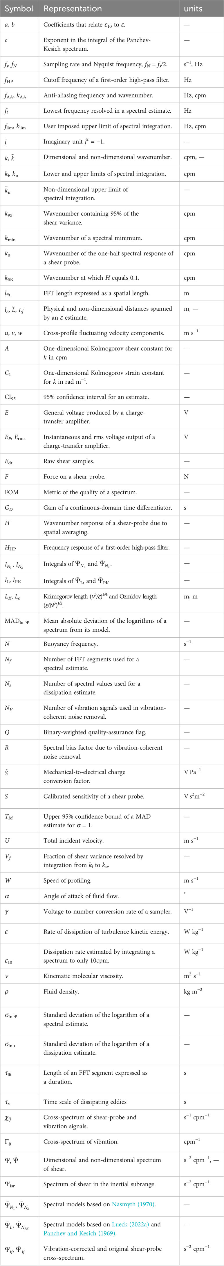
Table 1 A list of the symbols used in this contribution.
2 Background
2.1 Shear probes
The shear probe is an airfoil of revolution that was originally developed by Siddon (1965) for atmospheric and wind-tunnel measurements of turbulent cross-stream velocity fluctuations. The probe was subsequently modified for use in water (Siddon, 1971) and it was first deployed in 1972 on a vertical microstructure profiler in a fjord on the west coast of Canada (Osborn, 1974). Osborn and Crawford (1980) describe its theory of operation and one method of calibration. The sensing element is a two-layer piezo-ceramic beam that generates an electric charge in response to bending forces (Figure 1). About one-half of the beam is solidly anchored into its supporting stainless steel sting, and the other half is cantilevered out of the sting and will generate a charge when it is bent. The bending under a load is in the direction normal to the wide surface of the beam – much like a diving board at the side of a swimming pool bends in the vertical direction but not in the horizontal direction. A water-blocking layer is placed over the surface of the ceramic, and the entire tip is covered with silicon rubber to form a surface of revolution – much like the shape of a bullet. A piezo-ceramic responds only to time-varying fluctuations and produces no mean signal. Its high resistance ensures that the shear probe responds properly at and above the lowest apparent frequency of turbulent shear (f ≳ 0.1Hz). There are several versions of the shear probe. They differ mainly in the length of the tip measured relative to the point of the cantilever and the diameter at the point of the cantilever.
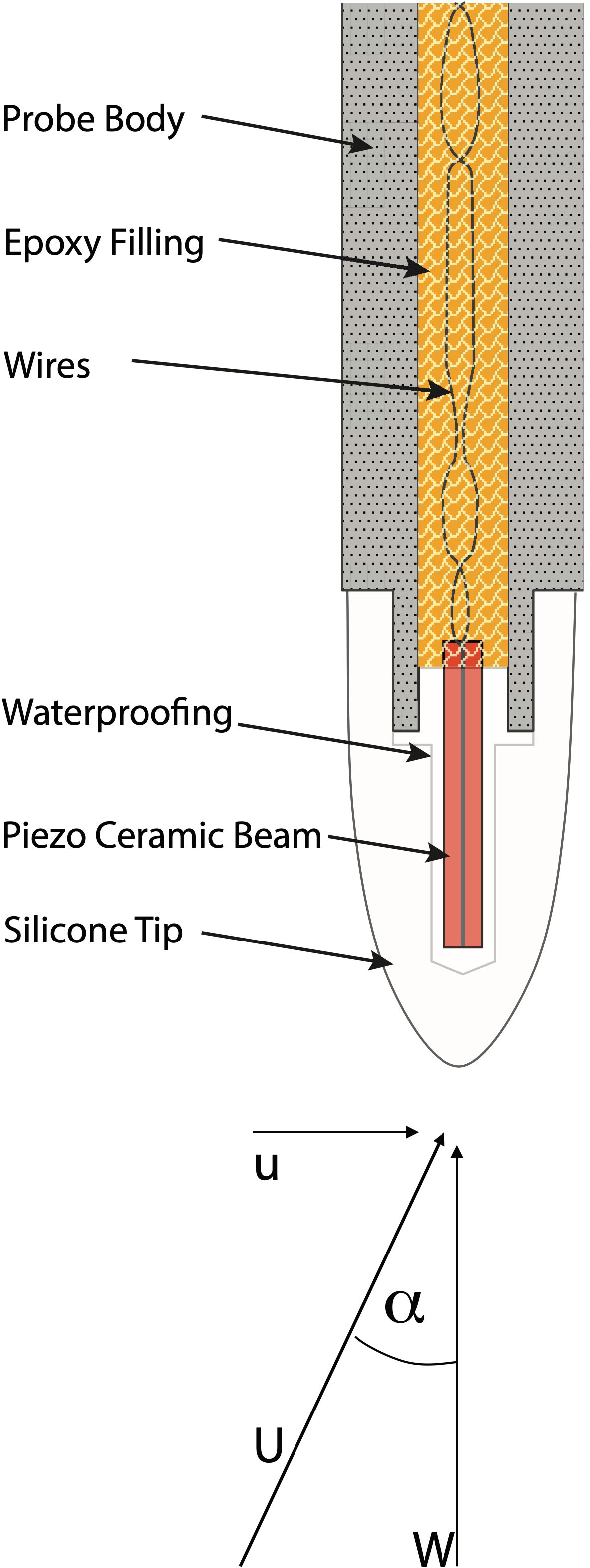
Figure 1 A sketch of the shear probe showing its main structural features and the expected incidental flow. The speed of profiling and the along-axis velocity is W, the cross-axis velocity is u, the angle of attack is α, and the total velocity is U. The force F of Equation 1 is directed along u. The typical outer diameter at the fulcrum of the beam is 5mm and the distance from the tip to the fulcrum is 9.5 mm.
Although the shear probe was initially used on vertical profilers, it can be used to measure the cross-profile fluctuation of velocity along any direction of profiling. Because there are always two orthogonal directions, profilers often carry two shear probes, with one rotated around its longitudinal axis by 90°, to measure both components of shear. Shear probes have been deployed on both downward and upward vertical profilers, on gliders that profile ≈30° with respect to horizontal (Fer et al., 2014; Palmer et al., 2015; St. Laurent, 2017), on towed and self-propelled vehicles (Fleury and Lueck, 1992; Osborn et al., 1992; Naveira Garabato et al., 2019), and on moored and fixed platforms where “profiling” is provided by the ambient current (Fer and Bakhoday Paskyabi, 2014; McMillan et al., 2016).
2.2 The signal produced by a shear probe
By the theory of potential flow past an axial-symmetric body, the across-axial force produced on the shear probe by a flow is
where U is the total incident velocity (Figure 1), α is the angle of attack, ρ is the fluid density, and u is the cross-axial component of the flow (Allen and Perkins, 1951). All velocities are relative to that of the probe because the probe senses only relative fluid velocity. The charge produced by the piezo-ceramic element is proportional to this lift force and, therefore, proportional to the cross-axis velocity u as well as to the along-axis velocity, W, i.e., the speed of profiling of the shear probe. Here we used an example of a vertical profiling instrument, hence adopting the notation W for the speed of profiling. However, we will use the symbol W for the speed of profiling regardless of its direction. The charge produced by the shear probe is converted into a voltage, E, by its supporting electronics and, thus,
where the factor depends on the efficiency of converting mechanical energy into electrical energy by the piezo-ceramic, the dimensions and shape of the probe, and the charge-to-voltage conversion of the electronics, and is determined through calibration.
One method of calibrating a shear probe is by exposing it to a jet of water with a velocity U and a time-varying angle of attack, α (Figure 1). The longitudinal axis of the probe is inclined by an angle α and it is spun around this axis to generate an angle of attack that varies sinusoidally with an amplitude α (Osborn and Crawford, 1980). The sensitivity of the shear probe is determined by regressing the root-mean-square voltage Erms against U2 sin2α so that
where the sensitivity, S, is the constant of proportionality. (When the shear probe was developed, it was easier to measure a root-mean-square voltage than a voltage amplitude.) The instantaneous voltage produced by the shear probe and its circuitry is then:
where the factor of comes from converting an rms voltage into a peak voltage. A typical value for S is 0.1 V m−2 s2. It is common to use the same charge-to-voltage converter during a calibration as the ones used in actual measurements.
2.3 Theories to estimate dissipation from shear spectra
In isotropic turbulence, the rate of dissipation, ε, is related to the variance of shear by
where the overline implies an average over a suitably chosen interval, ν is the temperature-dependent molecular kinematic viscosity of water (which ranges from 0.75 × 10⁻⁶ to 1.9 × 10⁻⁶ m2 s−1), Ψ is the spectrum of shear, k is the wavenumber, and kl and ku are the lower and upper wavenumbers of spectral integration (Taylor, 1935). Isotropic turbulence describes a state whereby the velocity components and their derivatives are independent of direction, i.e., they do not have a preferred orientation and appear similar from all points of view. The largest scale eddies of a turbulent flow contain the bulk of the turbulence kinetic energy of the flow and are usually not isotropic, while the smaller scales (the inertial and viscous subranges) are usually isotropic. The isotropic Equation 3 is valid for all six components of the shear. A typical shear spectrum (Figure 2) rises with wavenumber, k, in proportion to k1/3 in the inertial subrange (isr), and then diminishes rapidly with increasing k due to viscosity in the viscous subrange (vsr). In the inertial subrange, viscosity is not important, and its spectral form was first derived with a dimensional argument by Kolmogorov (1941). There is no first-principle-based theoretical prediction for the form of the shear spectrum in the viscous subrange – only empirical models and approximations.
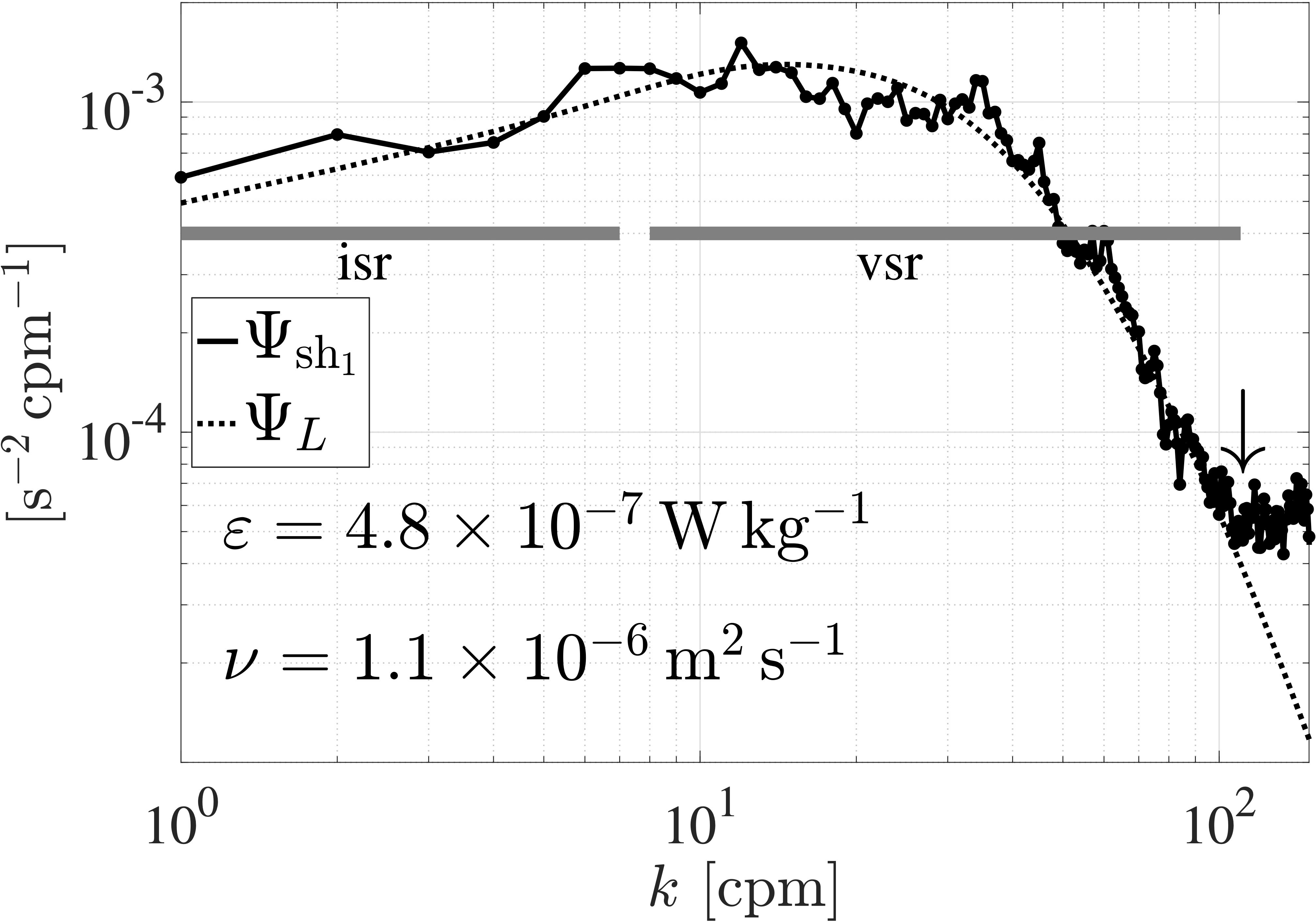
Figure 2 A typical spectrum of shear, , that has been corrected for spatial averaging and high-pass filtering, rises as k1/3 in the inertial subrange (isr), peaks, and diminishes in the viscous subrange (vsr). This spectrum rises past 100cpm (down arrow) due to electronic noise. ΨL is the approximation of Equation 7 for the indicated ε and ν.
Spectral models of shear are usually provided in a non-dimensional (often called universal) form, , and can be dimensionalized by using
where is the non-dimensional wavenumber and k is in units of cpm and dimensionalized using the Kolmogorov length LK(Figure 3). Note that the cyclic wavenumber k is different from the angular wavenumber which has units of rad m−1 and equals 2πk. The peak of the dimensional spectrum rises in proportion to ε3/4 (by virtue of the first line in Equation 4) and shifts to higher wavenumbers in proportion to ε1/4 (because of the second line in Equation 4), and this is required to make the area under the spectrum proportional to ε. As a result, the spectra of shear for high dissipation rates are not only higher, but they also span a broader range of wavenumbers. About 25% of the shear variance resides at wavenumbers smaller than the peak (Figure 3 diamond), and 95% of the shear variance resides at wavenumbers smaller than where the spectrum has dropped by a factor of 10 below its peak (Figure 3 right edge of shading).
Figure 3 The non-dimensional shear spectral models and their approximations in logarithmic (A) and in linear form (B). The solid lines are the spectra (red, Equation 5), (black, Equation 6), (maroon, Equation 7), (green, Equation 8). The dash-dot lines are the corresponding spectral integrals (Equation 9). The diamond marks the integral up to the peak of the spectra and equals ≈0.25. Wavenumbers smaller than the left edge of the gray shading contain 5% of the shear variance while those smaller than the right edge contain 95%. The dimensional wavenumber, k, is in units of cpm.
Four of the analytic approximations (or models) of the spectrum of shear are summarized here. The first is based on the values of the shear spectrum tabulated by Oakey (1982) that were derived from the along-profile velocity spectrum reported by Nasmyth (1970), and was originally approximated by Wolk et al. (2002) using:
who deemed the 8-th spectral value (counting from the lowest wavenumber and near ) to be erroneous because it is above the k1/3 tendency of the inertial subrange (Figure 3, red). The second is the approximation by Lueck (2022a) of the values tabulated by Oakey (1982) that includes the 8-th spectral value, namely:
(Figure 3, black). For this approximation, the values reported by Oakey (1982) were increased by 2% so that the integral of this spectrum equals 2/15 – a requirement for a spectral model of shear (Equation 3). The third is the spectrum proposed by Lueck (2022a) which is based on more than 14000 spectra of shear collected with shear probes, and is given by:
(Figure 3, maroon). The fourth spectrum is based on the three-dimensional velocity spectrum proposed by Panchev and Kesich (1969) which was converted into a one-dimensional shear spectrum by Roget et al. (2006) and reads:
(Figure 3, green). Note that rises more steeply than k1/3 at low wavenumbers. Because these approximations differ by only ∼15%, and because the statistical uncertainty of spectral estimates is usually larger by several factors of ten, any of these models can be used as a reference for comparison against a measured spectrum.
It is usually not possible to use the shear variance directly (in the time-domain) to estimate ε because of practical limitations such as electronic noise at high wavenumbers and vibrational contamination of the shear-probe measurements. Instead, ε is estimated by integrating the shear spectrum over a finite range of wavenumbers, i.e., by using the approximation in Equation 3). The lowest wavenumber is either kl = 0 cpm, or the lowest non-zero wavenumber, kl = (Wτfft)−1, where τfft is the length in seconds of an FFT segment used for a spectral estimate. The upper limit ku is detailed in Sec. 3.4.1. Limiting the bandwidth of the estimate allows for the exclusion of noise due to the electronics, vibrations, and other sources of contamination of the measurement of shear (see the high wavenumber end of Figure 2). However, limiting the bandwidth of an estimate of ε also excludes real shear variance and, therefore, an empirical model of turbulence shear is used to estimate the fraction of the variance that might be excluded. The approximations of the integral of the shear spectra of Equations 5 to 8 are
where c = 1.372 (Figure 3, dash-dot colored lines). The approximations of Equation 9 will be used in Sec. 3.4.1 to estimate the variance of shear that may be missing because of integration to a finite wavenumber, ku. Because of the similarity of the spectral approximations, any one of the integral models can be used for this purpose. In highly energetic environments (ε ≳ 10−5 W kg−1), such as in tidal channel flows, the upper ocean during storms, or vigorously turbulent overflows, the shear probe does not resolve the (high wavenumber) viscous subrange of the shear spectrum, because of the physical size of the probe. We thus recommended to fit the larger scales (lower wavenumbers) of the shear spectrum, which are within the inertial subrange, using a model spectrum that is based on the three-dimensional velocity spectrum proposed by Kolmogorov (1941) for the inertial subrange. This inertial-subrange shear spectrum is
where the coefficient C1 is the one-dimensional Kolmogorov constant for velocity fluctuations in the along profile direction (the strain component) and has an average value of C1 = 0.53 with a standard deviation of 0.055 (Sreenivasan, 1995). The Kolmogorov constant for the shear component is (Pope, 2009) and the factor of (2π)4/3 is required when working in units of cpm rather than rad m−1. The recommendation of Sreenivasan (1995) gives a value of A = 8.19, while the models and approximations of Equation 5 and Equation 7 give A = 8.05 and Equation 6 gives A = 7.89. These values span a range of ±2% and, therefore, all are suitable for estimating dissipation rates. However, in the inertial subrange, the model of Panchev and Kesich (1969) is not recommended because it does not rise as k1/3, which is inconsistent with the velocity spectrum proposed by Kolmogorov (1941) and the dimensional analysis of an isotropic spectrum in the inertial subrange.
The samples of a shear-probe signal are usually a time series and they are used to produce a frequency spectrum. A frequency spectrum is converted into a wavenumber spectrum by dividing the frequency by the speed of profiling, k = f/W, and by multiplying the frequency spectrum by W. However, this conversion is only valid if (i) the speed of profiling is reasonably steady over the time interval of a spectral estimate and (ii) the turbulence has not evolved during the time that it took to profile over the interval of an estimate. The second condition is often called the Taylor frozen field assumption. The time scale of dissipating eddies is τε∼ (ν/ε)1/2 and is of order 1s for a dissipation rate of 10−6 W kg−1. These two conditions place constraints on the interpretation of spectral estimates.
3 Recommended dissipation estimate procedure
The method described here is platform (or vehicle) independent and is summarized in the flow chart shown in Figure 4. The recommended procedure is presented in terms of levels, ranging from Level 1 to Level 4, where Level 1 is the data converted into physical units of shear, Level 2 is the selection, cleaning, and preparation of the shear data, Level 3 is its spectral estimation, and Level 4 is the estimation of the rate of dissipation, ε, from the spectra of shear and the quality control metrics that should accompany the estimates. These levels are abbreviated L1, L2, L3, and L4, respectively. The following subsections detail the recommendations for each step.
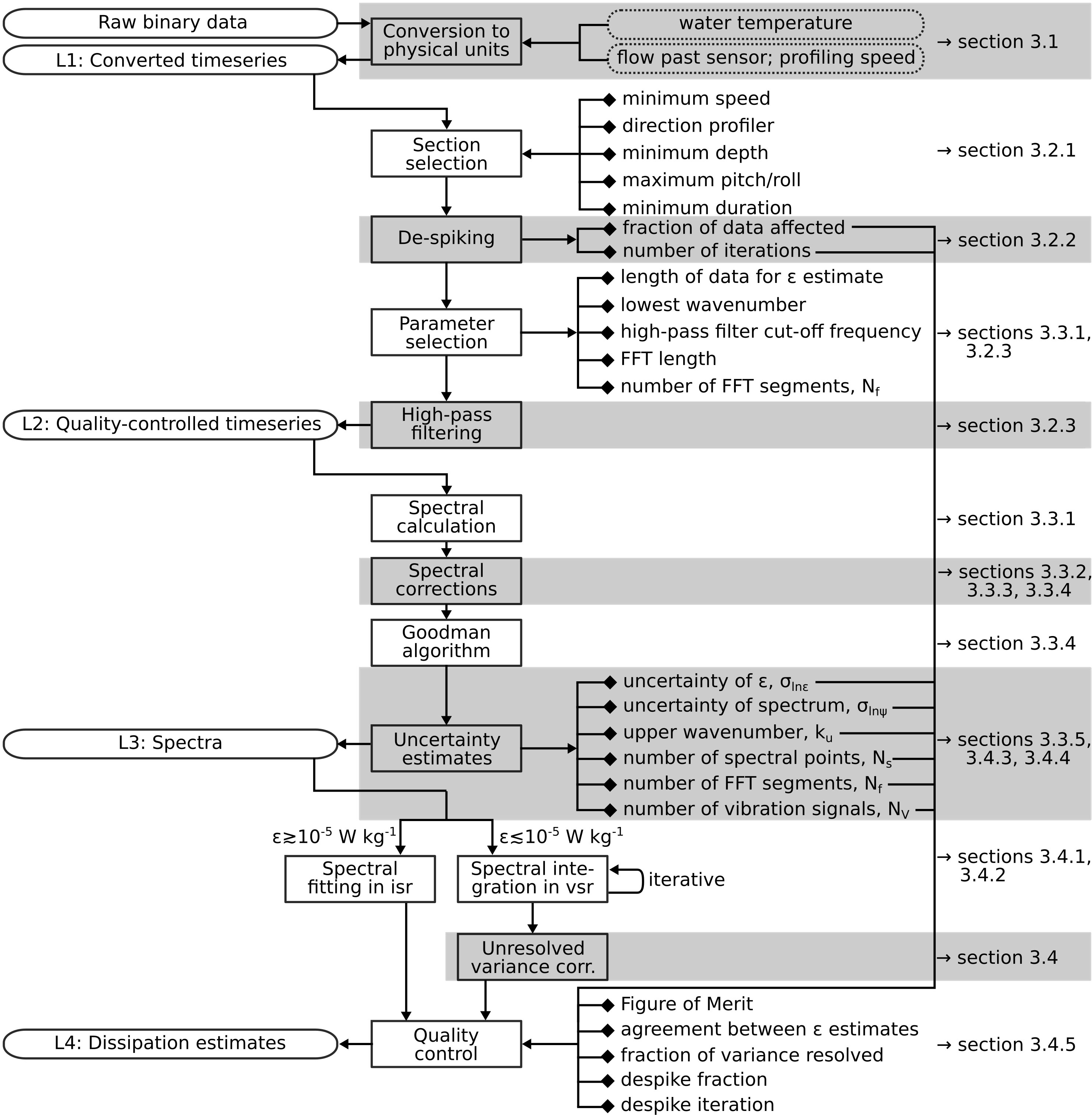
Figure 4 A schematic representation of the recommended processing of shear-probe data from L1 to L4. Details are provided in the sections shown on the right side.
3.1 L1: Obtain shear data in physical units
Data collected with a shear probe is always in the form of integers (whole numbers), produced by a sampler, that spans a range of values related to the voltage produced by the continuous-domain (analog) electronics that support the probe. The speed of profiling, W, is used to convert every whole-number sample into a value of shear. The speed may be available from one or more signals recorded by the instrument, or it may have to be determined from simultaneous measurements from another instrument. For example, when analyzing data collected from gliders, the flow past the shear probe and the angle of attack can be obtained from a hydrodynamic flight model of the glider, while for a vertical profiler, the rate-of-change of pressure may be used to deduce the speed of profiling. We emphasize that the rate-of-change of pressure only approximates the speed past the sensor when this speed is substantially larger than the background vertical velocity. This is typically valid for profilers ballasted for target speeds greater than ∼0.3m s−1, but can be invalid in regions where the magnitude of fluid vertical velocities are not small compared to W, for example, in tidal channels with energetic bottom-generated turbulence, in solitons, and within strong surface-wave orbital motions.
The cross-profile velocity signal produced by the shear probe (Equation 2) must be converted into a shear signal. In some instruments, this is done in the continuous domain by passing the signal through a time-differentiator electronic circuit, which is then sampled to produce
where GD is the gain of the differentiator in units of s, and γ is the voltage-to-number conversion rate of the sampler, and Edt are the shear samples. Finally, the discrete-domain signal of shear is derived using
The manufacturers of the electronics and the probes must provide the values of the differentiator gain, GD, the sensitivity, S, and the conversion rate of the sampler, γ. An estimate of the speed of profiling, W, is then used to complete the conversion of the dimensionless samples into a shear signal with physical units of s−1. Note that, for a given environmental shear, ∂u/∂z, the magnitude of the signal produced by a shear probe, Edt, is proportional to W2 and its variance, hence the dissipation rate, is proportional to W4. A consequence of this sensitivity to W is that a percent error in the profiling speed is amplified by a factor of four in the corresponding dissipation estimate. Furthermore, a higher than anticipated profiling speed, or exceeding the design speed of a profiler, can lead to signal overload and unreliable data.
It is also prudent to impose a minimum value on W in order to avoid infinities in (Equation 11). There is currently no consensus on a minimum value for W that still allows good measurements. The smallest value reported is W = 0.05m s−1 (Lueck et al., 1997). Experience indicates that data collected at speeds slower than 0.1m s−1 should be treated with suspicion.
For an instrument that does not electronically differentiate the continuous-domain shear-probe signal before sampling, the shear-probe data (i.e., the velocity, u), must be converted to shear in the discrete- or digital-domain using software numerical processing. This is achieved by one of two means. The first method involves taking the Fourier transform of the velocity samples, multiplying this transform by 2πjf where f is the frequency of the transformed samples, j2 = −1, and converting the multiplied transform back into the time domain using the inverse Fourier transform. This provides the rate of change of the velocity samples and is similar to that obtained by a continuous-domain differentiator. This signal can be converted into a shear signal by dividing it by the profiling speed. The second method of obtaining the rate-of-change of the sampled velocity signal involves using a first-difference operation, such as,
where fs is the sampling rate and n is the sample index. This is, however, only an approximation of a derivative that is asymptotically correct only in the limit of zero signal frequency and underestimates the derivative at higher frequencies. Spectra of shear derived from this approximation have to be recolored (adjusted with respect to frequency) by multiplying them by the factor
where is the Nyquist frequency, to account for the difference between the approximation of Equation 12 and a continuous-domain time derivative (Antoniou, 1979). This correction factor rises from unity at zero frequency to π2/4 ≈ 2.47 at the Nyquist frequency. In the method of processing discussed below, we assume that the samples represent a true time derivative and leave it to the user to make the spectral correction if they use a first-difference approximation to create a time derivative.
In addition, it may be necessary to make other spectral corrections if the manufacturer of the instrument modifies the frequency content of measurements in the band of interest for dissipation estimation.
3.2 L2: Prepare time series sections for analysis
3.2.1 Section selection
We must select segments within our data file (sections) that are suitable for analysis. A section is a continuous part of a time series that has been selected for dissipation estimates. For example, if the data come from an ascending profiler, only the data collected on the upcast are good for turbulence analysis. If the data were collected continuously while this instrument descended and ascended successively five times, the file could contain five data sections that correspond to the upward profiles. If an instrument mounted on a glider collected data continuously, the data from near to the turning points should be excluded from analysis. These times mark the boundaries of a section. During the turning of a glider, from ascent to descent and visa versa, the rate-of-change of pressure is small which makes it difficult to determine the speed of profiling. In addition, this is also a time of severe shaking of the glider by its buoyancy engines, which usually renders the shear-probe data unusable. If the profiling speed slows below the level of reliable probe operation (∼0.1m s−1) or the usable speed of a vehicle that carries the shear probe, new sections must be selected. This can happen, for example, when a glider stalls in response to strong current shear, during periods of weak currents or reversals in a moored system, and when the free-fall or free-rise of a vertically profiling instrument is interrupted by an operator or by strong updrafts in the water column. Thus, the shear time series in L2 can contain as little as a single section that lasts for only a few seconds, to as much as multiple sections that last for hours.
A measurement platform must satisfy certain threshold criteria for the measurements of shear to be valid for the estimation of the rate of dissipation. These criteria include a minimum speed of profiling, a maximum pitch and roll magnitude, a maximum acceleration magnitude, and a minimum depth. For a glider, there should also be a minimum pitch magnitude. These criteria must be satisfied for some minimum duration so that the section can produce at least one estimate of the rate of dissipation, ε. The response of the shear probe is fairly linear for angles of attack smaller than ∼20° (Osborn and Crawford, 1980). Pitching and rolling motions beyond this level will likely lead to non-linearity and other spurious effects and should be excluded from further analysis. As an example, when a vertical profiler is suspended near the surface over the vessel’s side, it will have a vertical velocity that oscillates around zero. Data collected at this time fails the speed and pitching criteria and so are unsuitable for analysis. After a profiling instrument is released, it will accelerate and reach ≈90% of its terminal fall rate in about one body length – a characteristic that may be slightly instrument dependent. Data collected during this period should also be excluded from analysis as it will fail the speed and acceleration criteria. The conversion of a frequency spectrum into a wavenumber spectrum becomes ambiguous if there are significant variations in speed during the interval used for a spectral estimate. Data collected during acceleration can be excluded by setting a minimum speed (80 to 90% of the known fall rate of an instrument) and a minimum depth that is more than two times the length of the profiler. Another suitable minimum depth must be deeper than the vessel’s draft used to deploy a profiler. This is because the vessel hull will likely disturb the water column. In quiescent conditions or using larger vessels, this minimum depth may be 1.5× the ship’s draft. If the measurement platform slows down below the minimum speed of the profiling threshold during data collection, a new section begins when the instrument reaches its terminal speed again for a minimum required duration. These conditions must be satisfied for a duration that equals the length of data we plan to use for each dissipation estimate divided by the speed of the profiler. The length of data record that should be used for an estimate of ε depends on a number of factors, including statistical uncertainty of an estimate (Sec. 3.3.5), and is often determined interactively as discussed below.
3.2.2 Cleaning shear-probe data
Collisions of the shear probe with plankton and other matter do occur and can greatly bias the variance of shear reported by a probe. Such encounters usually result in a “data spike” - a rapid rise (or fall), followed by a reversal, and a ringing with decaying amplitude, for a duration of ≈50 ms (Figure 5). Collisions with larger entities such as jellyfish and seaweed cause longer-lasting anomalies. Anomalous shear due to collisions must be removed from the shear-probe signals before spectral estimation. While different methodologies for de-spiking shear-probe signals are possible, we recommend the following algorithm to remove spikes effectively, using data from the whole L1 section (i.e., after removing unused data).
● Data are high-pass filtered, forwards and backwards, with a first-order Butterworth filter with a cutoff frequency of ≈0.1 Hz to remove offsets and very low-frequency signals without shifting the data in time.
● The data are rectified by taking their absolute value.
● A copy of the rectified data is smoothed by filtering it forwards and backwards, with a first-order low-pass filter with a cutoff frequency that is usually in the range of 0.25 to 2 Hz.
● Samples for which the absolute to the smoothed absolute shear ratio exceeds a threshold (typically 8), are identified as spikes.
● A number, N, of samples after a spike and N/2 before a spike are replaced by a constant value equal to the mean shear of an approximately one-half second interval before and after the range of replacement.
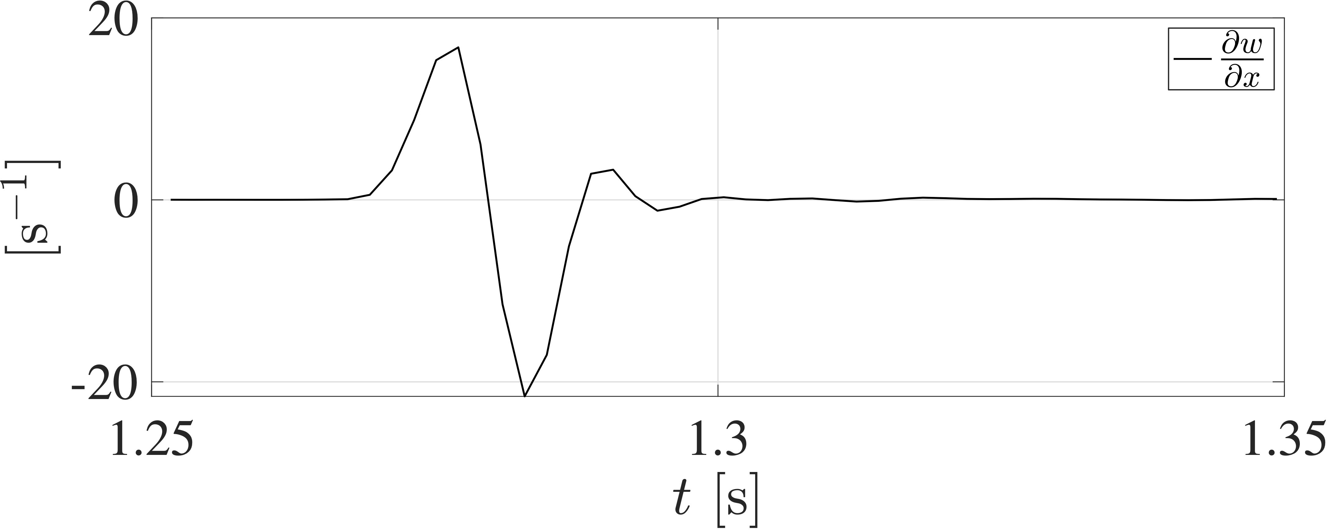
Figure 5 An example of a collision of the shear probe with zooplankton from a moored instrument.
These steps are repeated until there are no samples that exceed the threshold. The recommended algorithm and the choice of threshold values are based on experience. The purpose of the low-pass filter is to establish the typical magnitude of shear in a neighborhood that has a duration of approximately the inverse of its low-pass filter cutoff frequency. Forwards and backwards filtering imparts zero phase and no time-shift to the data. A shear sample is anomalous if its magnitude exceeds the typical magnitude by more than a factor of the threshold. Thus, if the variance of shear is small, a small anomaly is detected, while the same anomaly remains undetected if the variance of shear is large. That is, only anomalies that have the potential to bias the variance are removed. It is important to use a first-order filter because it does not cause over- and under-shoots, nor ringing, that could generate negative signals. We recommend that the parameters used for de-spiking be tested on actual data. The results are most sensitive to the choice of threshold.
What is a suitable neighborhood and low-pass cutoff frequency? Turbulent patches in the ocean are seldom thinner than about 0.5m in the vertical direction. This can serve as a lower limit to the definition of a neighborhood and an upper limit to the cutoff frequency. Thus, if a vertical profiler is moving at a speed of W, then the low-pass cutoff frequency should be no larger than ≈ W/0.5. Gliders that profile at an angle of ≈30° should use a cutoff frequency based on their vertical velocity rather than their profiling speed. Horizontal profilers should also use a value of ≈ W/0.5 because internal waves (and incomplete depth control) will likely cause it to undulate in and out of turbulent layers.
The response of the probe to a collision is a temporal one. A certain duration of shear data should be modified to remove the anomaly. Typically, the data are replaced 20 ms (i.e. around 10 samples for a sampling rate of 512 Hz) before a spike for the initial run-up to the first extrema and 40 ms (i.e. around 20 samples) after the last extrema for the decaying oscillation. The de-spiking should be applied iteratively to remove anomalies that last longer than 60 ms. The fraction of the data altered by a de-spiking routine must be noted for each data segment used to estimate a spectrum of shear because this is a quality-assurance metric. There is currently no standard for what is an acceptable fraction of modified (de-spiked) data.
Usually, for a good dissipation rate estimate, the fraction of data altered by de-spiking is smaller than ≈2%. However, there are circumstances when the fraction may exceed this value. Examples include (i) when profiling during a spring bloom when the density of zooplankton and other small creatures may be very high and (ii) when the shear probes are mounted on instruments (such as gliders and other autonomous vehicles) which use actuators that impart strong mechanical impulses. For such cases, an upper limit of 5% may be more appropriate for quality control.
The number of passes or attempts made to clean the shear-probe data is also a quality-assurance metric. Note that the cleaning of the shear probe data is exercised only in the selected section satisfying the profiling criteria of Sec. 3.2.1 and, hence, it excludes times of excessive platform motion, vibration, acceleration, tilt, or slow relative speed past the probes. If many attempts are required to clean the data, then the anomalies are extremely long and may be caused by collisions with objects larger than the typical size of zooplankton such as, for example, jellyfish. While there is no objective criterion for the maximum number of passes that should be tolerated, experience indicates that data requiring more than 8 passes are very unusual and should not be used for the estimation of the rate of dissipation.
3.2.3 High-pass filter time series
Although the shear probe inherently senses only zero-mean fluctuations, its electronics may impart a non-zero mean that should be removed by digital high-pass filtering. Once the data have been cleaned by removing shear anomalies, it can be filtered. The cutoff frequency for digital high-pass filtering must be decided at this stage. The recommended high-pass filter is a first-order Butterworth filter, applied forwards and backwards, with a cutoff frequency of approximately one-half of the lowest frequency resolved by the spectra for dissipation estimates. The lowest frequency resolved is , where τfft is the length of the FFT segments (in s) (see Sec. 3.3.1). Thus, the recommended choice for high-pass filtering of the shear data is
3.3 L3: Produce wavenumber spectra of shear and related sensors
The shear variance is obtained from a wavenumber spectrum of a shear time series that is cleaned (de-spiked) and high-pass filtered as described earlier. Here we describe (i) how the wavenumber spectrum should be calculated, (ii) its correction for the high-pass filter, and (iii) the removal of vibration-coherent contamination.
3.3.1 Spectral calculations
The estimation of spectra and dissipation rates requires setting a number of parameters that determine both the spatial resolution of the dissipation estimates and the statistical reliability of the estimates of the shear spectrum. A duration of data, τε, will be used to estimate ε. This duration is divided into a number of shorter FFT segments of duration τfft. By the periodogram method of spectral estimation, the magnitude squared of the Fourier transform of the FFT sections is averaged into a single magnitude-squared transform, at each frequency between zero and the Nyquist frequency. This averaged transform is divided by both the number of points within a single FFT segment and by the Nyquist frequency to make it equal to a spectrum – its integral equals the variance of the shear signal. The spatial resolution of the dissipation estimates is lϵ = τεW and is a choice driven by scientific objectives, such as the spatial resolution required to reach your objectives. The resolution (and the lowest non-zero wavenumber) of a spectrum is kl = fl/W = (τfftW)−1 and must be chosen carefully by considering the constraints below.
Spectra must resolve the peak of the spectrum and a portion of the inertial subrange in order to confirm that they represent shear, and this sets a dissipation rate dependent requirement on the minimum length of an FFT segment. Spectra for dissipation rates that are low (ε ≲ 10−9 W kg−1), moderate (ε ≲ 10−7 W kg−1), and high (ε ≳ 10−7 W kg−1), are well resolved by kl equal to ≈0.5, ≈1, and ≈2 cpm, respectively. For an instrument with a slow profiling speed of W = 0.3m s−1, an FFT length of τfft = 7s is needed to resolve kl = 0.5 cpm, whereas a profiling speed of 1m s−1 requires an FFT length of only 2s.
An FFT length converted to a spatial length, lfft = τfftW, should not exceed the length of a free profiler because the profiler will be advected by eddies comparable to and larger than the profiler, which diminishes the large-scale shear measured by the shear probe. For example, an FFT duration of τfft = 2 s and a profiling speed of W = 0.5m s−1 gives a spatial length of 1m, and this value should be comparable to or shorter than the length of a free profiler.
The FFT segments should be individually detrended by either a zero-order or a first-order polynomial to minimize the zero-frequency spectral value (which is assumed to be zero) and to reduce the leakage of low-frequency content into the first non-zero frequency spectral estimate. Higher-order detrending removes low-frequency variance and is not recommended.
Because turbulence shear is a broad-banded signal (one with a spectrum that does not change rapidly with respect to wave-number), the detrended FFT segments should be windowed and overlapped to increase the statistical reliability of the spectrum. Here, windowing means multiplying the time series record in the FFT segment by a window shape that varies smoothly from zero at the start of a segment, reaches a peak, and decreases symmetrically to zero at the end of the segment. It is important to do both. Neither windowing without overlap nor overlapping without a window increases the statistical reliability of a spectrum (Nuttall, 1971). The actual window used is not critical but it must be scaled to have a mean-square equal to 1, so that it does not change the variance of the signal. We recommend a cosine window with 50% overlap between adjacent segments. Thus, a data length that is twice as long as the FFT length uses three FFT segments (Nf = 3) for the spectral estimate and this ratio should be considered a minimum, unless there is a pressing need for very high spatial resolution of the ε estimates. The statistical reliability of a spectrum can be increased by increasing the length of data, lε, used for a dissipation estimate because that increases Nf for a fixed length of an FFT segment (Equation 17). However, an increase in lϵ must be tempered by the assumption of stationarity over the length of an estimate. Large values of Nf can invalidate the stationarity assumption, particularly in boundary layers where dissipation rates can change rapidly with depth, or in parts of the time series with substantial acceleration or deceleration of profiling speed.
Finally, if a high spatial resolution of dissipation estimates is important to reveal variations, then it is also possible to overlap successive estimates of ε. This makes successive estimates statistically interdependent but it may be useful for revealing patterns of dissipation rates.
3.3.2 Correction for the spatial response
The shear probe has a frequency response determined by the probe tip’s mechanical stiffness and mass. Vibration tests indicate that the frequency response is several kilo-hertz and, therefore, not an issue at the usual speeds of profiling. However, its finite size does induce spatial averaging which limits the wavenumber response of the shear probe. Macoun and Lueck (2004) indicate that the response of their probes has the form of a first-order low-pass filter with a half-power wavenumber of k0 = 50 cpm. That is, the measured spectrum is reduced by the factor
where k is the wavenumber in units of cpm. This response was determined for a probe with a length of 9.5 mm from tip to fulcrum and diameter of 5 mm at its fulcrum. The response scales with the size of the probe and may be different for other probes. Spectra of shear must be multiplied by the inverse of Equation 14 to correct them for the spatial averaging by the shear probe. Note that this correction amplifies the spectrum by a factor of 10 at a wavenumber of 150 cpm, and it is not recommended to use the spectrum at wavenumbers where the correction exceeds a factor of ≈10 because k0 has some uncertainty and excessive boosting amplifies this uncertainty and transfer it into the spectrum and the estimate of ε.
3.3.3 Correction for high-pass filter
Digital filters are not perfect as they attenuate the spectra at frequencies smaller and larger than the cutoff frequency. The spectra should be corrected for the first-order, high-pass filter applied both forwards and backwards at L2. The spectral correction is the inverse of the magnitude-squared response of such a filter which is:
where fHP is the high-pass cut-off frequency (Antoniou, 1979). For the recommended high-pass cut-off frequency of Equation 13, namely , the correction at the lowest (non-zero) frequency of the spectrum, namely , is only a factor of (5/4)2, and this factor diminishes rapidly to unity with increasing frequency.
3.3.4 Vibration-coherent noise removal
If there are concurrent measurements of the acceleration, or the vibration, of the platform that carries the shear probes, then these measurements should be used to remove those parts of the shear signals that are coherent with the vibrations. (A vibration sensor measures only the time-varying part of an acceleration.) We recommend that the accelerometer and shear-probe signals are sampled at the same rate. If the signals are not sampled at the same rate, and if the lower of the two Nyquist frequencies covers the band of interest for the shear spectrum, then interpolation may be used before the coherency calculation. For the vibration-coherent noise removal, we recommend the method of Goodman et al. (2006), which removes multi-variate coherent vibrations from a multi-variate shear spectrum using
where Ψij and are the corrected (de-contaminated) and original cross-spectrum of the i-th and the j-th shear-probe signals, χij is the cross-spectrum of the shear-probe and vibration signals, Γij is the crossspectrum of the vibration (and possibly other) signals that are contaminating the shear-probe measurements, the superscript ∗ indicates a complex conjugate, and summation over repeated indices is implied. All of these quantities are functions of frequency (or wavenumber).
The term ‘cross-spectrum’ needs some clarification. The cross-spectrum of the i-th and the j-th shear-probe signals is a three-dimensional and complex matrix that has dimensions of P × P × N where P is the number of shear signals, and N is the number of frequency indices in the cross-spectrum. The auto-spectra of the shear signals are on the diagonal of this three-dimensional cross-spectrum. For example, Ψ22(f) is the auto-spectrum of the signal from shear probe 2. It is real. The off-diagonal elements are the cross-spectra between pairs of shear probes. For example, is the cross-spectrum of probes 1 and 2. It is complex. The cross-spectrum of vibrations, Γij, has dimensions M × M × N where M is the number of vibration signals that are used to remove coherent noise from the shear-probe signals. The cross-spectrum of the i-th shear-probe and the j-th vibration signals, χij, has dimensions P × M × N, and is entirely complex.
The technique of Goodman et al. (2006) relies on estimating the (squared-) coherency between the vibration and shear-probe signals. The second term on the right-hand side of Equation 15 is the coherency times the cross-spectrum of shear. Coherency is a positive definite quantity and is always finite, even for completely unrelated signals, when the number of FFT segments used to make its estimate is finite. That is, it underestimates the corrected spectrum Ψij(f), at all frequencies, by a factor of
where NV < Nf is the number of vibration (and other) signals used to remove vibration-coherent noise from the shear-probe spectra, and Nf is the number of FFT segments used to make the estimate (Ferron et al., 2023). The spectrum of shear is corrected by dividing it by R. The factor of 1.02 in Equation 16 was determined empirically for a cosine window with 50% overlap. However, it is nearly identical for other windows and for all overlaps that are smaller than ≈ 2/3. For the example (Sec. 4.1) Nf = 7 and using three vibration sensors NV = 3, we obtain R = 0.563. The technique of Goodman et al. (2006) will not work unless Nf > NV and, preferably, larger by more than 3 for reasons of statistical reliability (Sec. 3.3.5).
3.3.5 Uncertainty of a shear spectrum
The statistical reliability of an estimate of a spectrum of shear has a probability density function (pdf) that is log-normal, and has been explored by Lueck (2022a). The statistical uncertainty of an estimate of the natural logarithm of the spectrum of shear has a variance of:
3.4 L4: Dissipation estimates from spectra
3.4.1 Estimating ε by spectral integration
A common method of estimating ε is by integrating the shear spectrum between a low and high wavenumber limit. Particularly, the choice of the upper wavenumber limit of spectral integration must be made after careful considerations described below. Estimating the variance of shear, and hence ε must be done iteratively because the bandwidth required for an estimate, i.e., wavenumber limits of integration, is a priori unknown because it depends on the value of ε itself. Very small dissipation rates ≲ 10−10 W kg−1 are well resolved by a bandwidth of ≈10 cpm. Often vibrations and other sources of signal contamination are small for wavenumbers smaller than ≈10 cpm. Thus, integrating a spectrum to 10cpm can provide an initial estimate of ε if the spectrum conforms reasonably closely to a model spectrum such as that by Nasmyth (Figure 3, black line). The limit of 10cpm was also suggested by Wesson and Gregg (1994) as a means to make an initial estimate of ε. The ratio of the actual dissipation rate, ε, to that estimated by integrating a spectral model (such as Equation 6) to only 10 cpm, ε10, is well approximated by:
(Figure 6). The likely underestimated rate of dissipation, which is derived by integrating a measured (and cleaned) spectrum to 10 cpm, can then be boosted by Equation 19 to make an improved estimate of the rate of dissipation, denoted ε1. According to most models, 95% of the variance of shear is resolved at a non-dimensional wavenumber of (Figure 3). Thus, k95 = 0.12(ε1/ν3)1/4, in units of cpm, is a suitable upper limit for the integration of a shear spectrum. There is little point in integrating beyond this wavenumber because the correction for the missing variance is only 5%. If integrating to 10cpm is not convenient, then a boosting relationship such as Equation 19 should be developed for other spectral limits to derive an initial estimate of ε1.
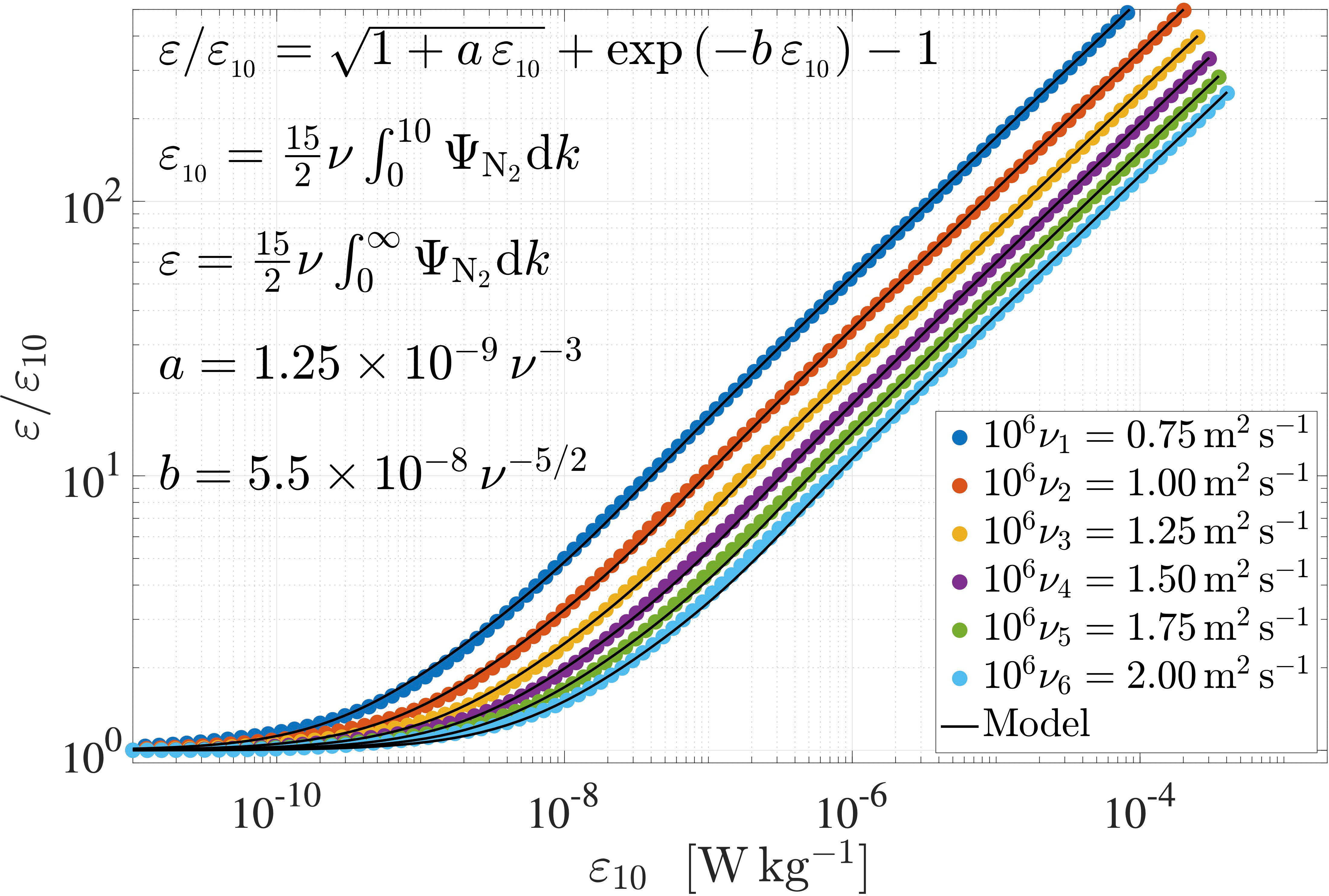
Figure 6 The rate of dissipation, ε, according to the Nasmyth model spectrum of Equation 6, relative to an estimate based on integrating this spectrum to 10 cpm, ε10, as a function of ε10 for a range of viscosity, ν (colored disks) and an analytic approximation (black line).
Electronic noise sets another upper limit for spectral integration. Because of the differentiator operator in obtaining shear, either done electronically in the signal chain or applied during post-processing of the velocity time series, the noise in the spectrum of shear tends to rise with increasing wavenumber (Figure 2, down arrow). The wavenumber at which this spectral minimum occurs depends on ε. For very low dissipation rates, the minimum occurs at low wavenumbers because the level of the spectrum rises in proportion to ε3/4, while the spectrum of electronic noise is constant at a given speed. For very high rates of dissipation, the spectral minimum may not even appear because the electronic noise may be smaller than the shear signal at all wavenumbers. The spectrum of shear should not be integrated beyond the spectral minimum so that the estimate of the variance of shear is not biased high by electronic noise. The spectral minimum can be found by fitting a polynomial to the spectrum in log-log space. A fit of order 3 is often sufficient to find the spectral minimum but odd orders up to 7 also give satisfactory results. In most cases, the fit should be of an odd-numbered order because the typical shape of a spectrum, with respect to increasing wavenumber, is a rise from the lowest wavenumber to a peak, a subsequent decrease due to viscosity, and a final rise due to noise. The spectral minimum is between the fall due to viscosity and rise due to electronic noise – for example, the down arrow in Figure 2. This sort of shape is emulated by an odd-order polynomial. To avoid the detection of false minima, the minimum determined from a polynomial fit should not be smaller than 10cpm because at this wavenumber a spectrum is about 95% resolved when the rate of dissipation is very low, ∼10−10 W kg−1. We denote the wavenumber of the spectral minimum by kmin.
Another limit is due to the shear probe’s limited wavenumber response (Equation 14). We do not recommend integrating the spectrum beyond the wavenumber at which the spectral correction (for spatial averaging by the shear probe) exceeds a factor of 10. This is not a hard limit but spectra corrected by a factor much larger than 10 are unreliable because the correction itself has some uncertainty. We denote this limit due to spatial resolution by kSR. It equals 150 cpm for the probes used by Macoun and Lueck (2004) and should be determined for other probes if they differ substantially from their probes.
Most data acquisition systems apply a low-pass filter to the continuous-domain shear signal before sampling to suppress aliasing. This is done in the continuous domain with a filter that has a cutoff frequency of fAA. The spectrum is unresolved beyond this frequency. Therefore, another upper limit to spectral integration is kAA= 0.9 fAA/W where the factor of 0.9 is used to avoid the transition from the pass band to the attenuation band of the anti-aliasing filter. This factor is suitable for an 8-th order Butterworth filter. Sharper filters can have a factor closer to unity, while filters of a lower order, or ones of a wider transition range, should use a factor that is smaller than 0.9.
Finally, there may be some corruption of the shear spectrum that is not removable but, if it is included in the spectral integration, it will bias high the estimate of the shear variance. This sort of spectral contamination is an instrument or an operational problem that should be corrected. If present, the contamination usually occurs at a (nearly) fixed frequency and, thus, this limit is usually specified in terms of frequency rather than wavenumber. If the spectrum is good for frequencies lower than flim, then another limit of spectral integration, is klim = flim/W. For good data, flim should be set to infinity so that it is irrelevant.
In summary, the various upper wavenumber limits of spectral integration are:
● k95 = 0.12(ε1/ν3)1/4 – the wavenumber of 95% resolution,
● kmin – the wavenumber of the spectral minimum,
● kSR – the wavenumber (typically 150cpm) of the factor of 10 correction for spatial resolution,
● kAA– the wavenumber corresponding to the cutoff frequency of the anti-aliasing filter, and
● klim – the wavenumber of irremovable spectral corruption.
The spectrum of shear can now be integrated to estimate the variance of shear and to derive the second estimate of the rate of dissipation, ε2. For this estimate, the spectrum should be integrated to an upper limit equal to the smallest of the five cited upper limits. That is ku = min(k95, kmin, kSR, kAA, klim). The upper limit ku will usually be larger than 10cpm and, therefore, the estimate ε2 derived by integration to ku will be statistically more reliable than the initial estimate, ε1. However, the spectrum is not fully resolved at ku and ε2 will be an underestimate because some shear variance will be excluded.
The estimated ε2 is then used to estimate the non-dimensional value of the upper wavenumber of spectral integration, namely
This value is used with one of the models of the integral of a spectrum (Equation 9) to estimate the fraction of the shear variance that is resolved by integrating the spectrum to ku. For example, the resolved fraction is , and an improved estimate is
We recommend using zero as the lower limit of spectral integration, kl = 0 cpm, and setting its spectral value to zero, because that is the expectation of the spectrum – which rises as k1/3 at low wavenumbers. Algorithms that estimate the variance of shear by integrating the spectrum from a non-zero lower wavenumber, kl > 0 cpm, have to correct their estimate for the exclusion of variance below their lower limit of spectral integration and this can be done with any of the models in Equation 9. In stratified turbulence, eddies with a size comparable to and larger than the Ozmidov scale, LO = (ε/N3)1/2 where N is the buoyancy frequency, are damped by stratification. One could choose a lower wavenumber of spectral integration equal to . However, choosing such a lower limit has only minor consequences because there is little variance below because of the damping by buoyancy. Using the Ozmidov length for a lower limit must be made iteratively because it depends on ε.
The integration of the spectrum is usually done by the trapezoidal approximation of an integral. This introduces a slight error in the low wavenumber range. The spectrum is expected to rise as k1/3 from a wavenumber of zero to at least the first non-zero wavenumber, k1. This makes the integral equal to 3k1 Ψ(k1)/4. However, the trapezoidal approximation gives k1 Ψ(k1)/2 which is smaller than a true integral. An amount equal to k1 Ψ(k1)/4 should be added to the estimated variance to correct this shortfall when using kl = 0.
The spectra used for estimating ε by spectral integration must be corrected for the wavenumber response of the shear probe, the high-pass filter that is applied to remove spurious low-wavenumber variance, any other wavenumber dependencies that may be inherent in the measurement system, and for the bias induced by vibration-coherent noise removal.
With the method of spectral integration, we are estimating the variance of shear and using it to derive ε because they are related by first principles (Taylor, 1935). For typical dissipation rates (ε ⪅ 10−5 W kg−1), we do not recommend fitting the measured spectrum to a model spectrum to derive a dissipation estimate because there are no spectral models that are based on first principles. Model spectra are only used to estimate the fraction of the variance that is excluded by a finite upper wavenumber limit of spectral integration, and possibly a lower limit if integration does not start at 0cpm. However, if measured spectra are close to model spectra, then spectral fitting and variance estimation give similar results. The computational burden of spectral fitting is, however, much higher.
3.4.2 Estimating ε by fitting to the inertial subrange
When dissipation rates are very high, ε ≳ 10−5 W kg−1, the shear probe cannot resolve the spectrum of shear and even the wavenumber correction proposed by Macoun and Lueck (2004) does not produce spectra that agree closely with spectral models. However, the shear probe always resolves the inertial subrange, for oceanic conditions, which has wavenumbers smaller than k< 0.01(ε/ν3)1/4 in units of cpm, and this range can be estimated with the value of ε1 derived from the spectral integration to 10cpm. Fitting the spectrum in the inertial subrange provides an alternative method to spectral integration. The model spectrum in the inertial subrange is given by Equation 10.
The actual fitting method is not crucial. One method that gives satisfactory results is to use ε1 (derived from a spectral integration to 10 cpm) to delineate the inertial subrange. The ratio of the observed and model spectral values is then computed and averaged over the subrange. The rate of dissipation of the model spectrum (Equation 10) is adjusted until the average ratio equals unity (to within, say, 1%). This method is the same as log-transforming the inertial subrange model and solving this relation
over the inertial subrange, where Ψ(k) is the observed spectrum. The minimum number of spectral values that must be used for a fitting is not well established. Equation 20 is equivalent to the ‘null model’ examined by Jenkins and Quintana-Ascencio (2020) who recommend a minimum of 5 points.
Because the inertial subrange is only a small part of the entire spectrum of shear, the number of spectral values used for a dissipation estimate by a fit to the inertial subrange is almost always smaller than the number of values used in spectral integration. Consequently, the statistical reliability of such an estimate is inferior to that obtained by integration. However, when dissipation rates are high, ε ≳ 10−5 W kg−1, spectral integration is not an option because the shear probe cannot resolve the spectrum, and integration provides an underestimate of ε.
The spectra used for estimating ε by fitting in the inertial subrange must also be corrected for the high-pass filter that is applied to remove spurious low-wavenumber variance, for the bias induced by vibration-coherent noise removal, and for the wavenumber response of the shear probe, although this correction will usually be minor.
3.4.3 Uncertainty of an ε estimate by spectral integration
The statistical uncertainty that we present here is that of a measurement uncertainty that is due to the limited sampling of a statistical process (the turbulence shear) to estimate its variance and spectrum. The underlying statistical uncertainty of a dissipation estimate is presented in Lueck (2022b), and the uncertainty of a spectral estimate is in Lueck (2022a). The measurement uncertainty is distinct from the uncertainty of how a particular estimate relates to the longer-term average of ε at a particular site. The uncertainty of an ε estimate is different for methods of spectral integration and fitting in the inertial subrange and must be carefully calculated. When the rate of dissipation is estimated by spectral integration, the statistical uncertainty of the logarithm of such an estimate has a variance of:
where lε = τεW is the length (in units of m) of data used for the dissipation estimate, LK is the Kolmogorov length, and Vf is the fraction of the shear variance resolved by ending the spectral integration at a finite wavenumber of ku (Lueck, 2022b). The non-dimensional data length, , is reduced by a factor of 4 because samples of shear are independent only if they are separated by more than four Kolmogorov lengths, where the lagged auto-correlation of shear drops to one-half (Lueck, 2022b). The factor of Vf accounts for the underusage of information because of limiting the spectral integration to k ≤ ku. Thus, the 95% confidence interval for a dissipation estimate derived by spectral integration is:
In L4, every estimate of ε should be accompanied by its value σlnε, lε, LK, and Vf, if the estimate was made by spectral integration, as explained in Sec. 3.4.1.
3.4.4 Uncertainty of an ε estimate by fitting in the inertial subrange
The method of fitting a spectrum in the inertial subrange to a model spectrum is equivalent to finding the average of Equation 20 for the spectral values in the inertial subrange. The logarithm of each spectral value has a variance of Equation 17. If there are Ns spectral values in the inertial subrange used for a spectral fit, the variance of the average logarithmic differences is smaller by a factor of Ns. Thus, the 95% confidence interval of is:
and the same confidence interval for ε itself is
In L4, every estimate of ε derived by fitting in the inertial subrange should be accompanied by its value of Ns, so that one can place a confidence interval on this estimate using Equation 21 and the value of σlnΨ that is located in L3 (Sec. 3.3.5). The value of Ns is also pertinent to quantifying the quality of a spectrum (Sec. 3.4.5).
3.4.5 Quality-assurance metrics
The quality of a dissipation estimate, and the spectrum from which it is derived, must be quantified and must accompany each estimate. This is a requirement imposed by data archives. We propose five quality-assurance metrics and a single flag value, Q, that can be used to identify a failure of any combination of these metrics. The quality-assurance metrics are combined into a single Q flag value by combining bit-wise values, of 0 or 1 corresponding to base-2 numerals of 1, 2, 4, 8, and so on, into a single multi-bit number. For example, a value of Q = 0 means that the estimate passed all metrics, while a value of Q = 5 uniquely identifies that the estimate failed both metric numbers 1 and 4. Failures increase the value of Q by the amounts described below. The quality-assurance values are summarized in Table 2. When dissipation estimates are made using more than a single probe, the final estimate should be the average of those estimates that have Q = 0.
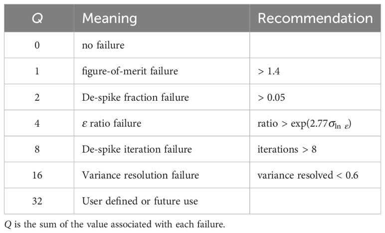
Table 2 Summary of the values of the Q flags associated with the quality-assurance metrics, and the recommended values for conditions for their failure.
3.4.5.1 Poor figure of merit (Q = 1)
Figure of merit (FOM) is a measure of the quality of a spectrum, over the range of wavenumbers that is used for the estimation of ε. The FOM provides a measure of how closely a spectrum agrees with a model spectrum and, therefore, it is appropriate only for cases where the assumptions that underpin the model spectra are valid. The assumptions of the model spectra are (i) that the turbulence is isotropic, (ii) that there is a flow of energy from large to small scales, and (ii) that the generating scales are very much larger than the dissipating scales. The standard deviation of a spectrum, Equation 17, has only been tested for buoyancy Reynolds number:
and may not apply to regions with weaker turbulence or stronger stratification. In addition, shear fluctuations that are generated by fauna or other biological activity, salt fingers, or are extremely close to boundaries may not have spectra that are similar to the model spectra.
To derive the FOM statistic, we start by assembling the difference between the natural logarithm of the measured spectrum, ln Ψ, and the natural logarithm of a model spectrum, ln ΨM, that has been dimensionalized using the estimated ε and the known kinematic molecular viscosity, ν. We then calculate the mean absolute difference (or deviation) using only the spectral values in the range of wavenumber that were used to estimate ε. That is, we calculate:
where i are the indices to the Ns spectral values that were used for a dissipation estimate. This excludes the index to k = 0 cpm because that spectral value is prescribed to be zero. This sample MAD must be compared to the mean absolute deviation that is expected from the known standard deviation of the spectrum, σln Ψ (Equation 17). If a zero-mean normal population has a standard deviation of σ, then its expected MAD is 0.8σ. However, a sample MAD based on Ns samples will have a range of values around this expectation of 0.8σ and this range has an upper 95% confidence interval of:
where
was determined by calculating the 95% confidence range of a large number of MAD estimates using samples drawn from a normal population with a standard deviation of 1 (Figure 7). Thus, we expect that for 97.5% of spectra the figure of merit:
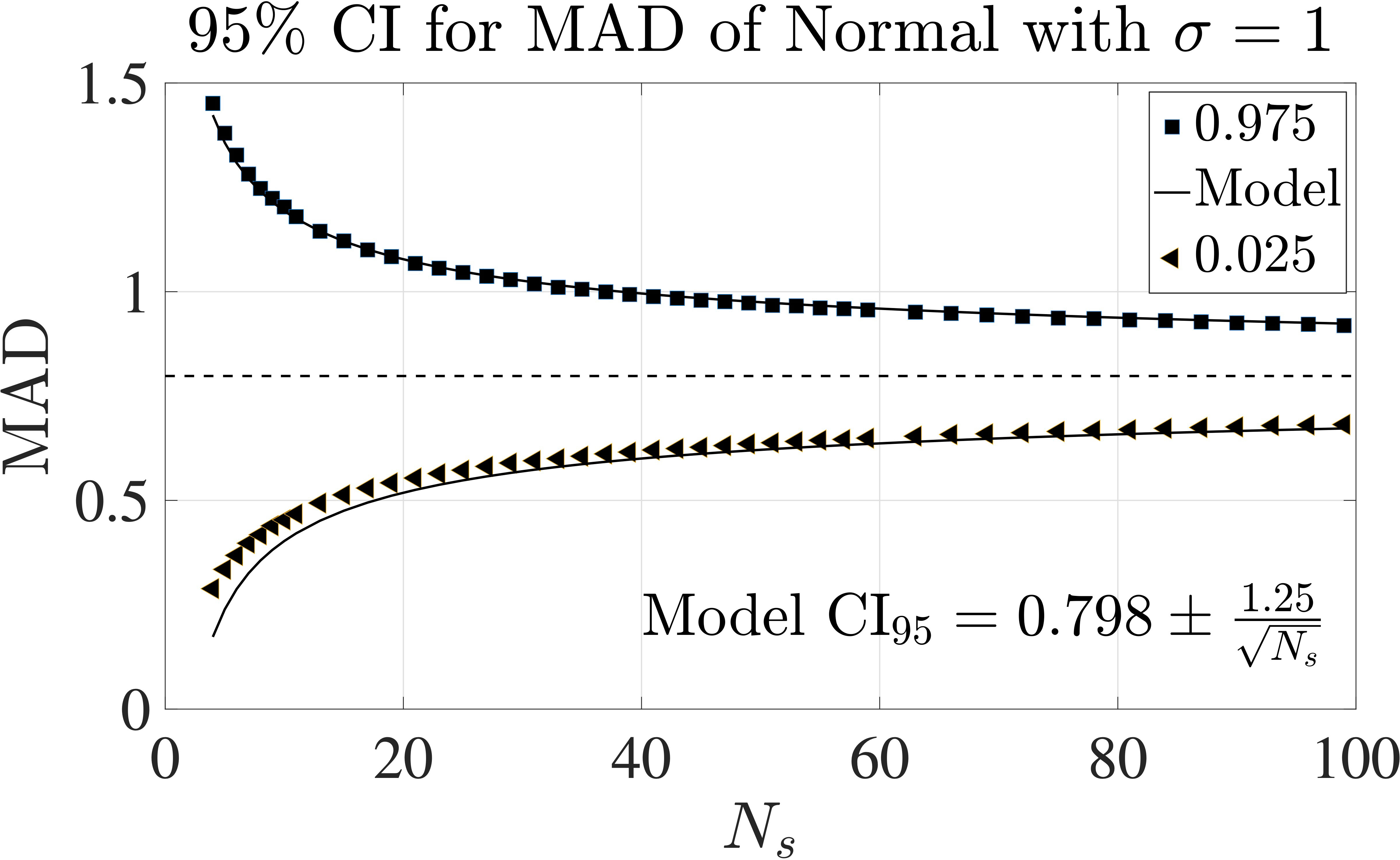
Figure 7 The 95% confidence interval of the mean absolute deviation (MAD) of Ns samples drawn from a normal population with a standard deviation of σ = 1. The analytical model approximation is from (Lueck, 2022a).
to be smaller than 1 if the model spectrum, ΨM, is an appropriate expectation for the measured turbulence. Perfect agreement between a measured and a model spectrum has FOM = 0, and 2.5% of spectra have FOM > 1. However, there is an approximately 15% difference among the four spectral models and, so, the threshold should be increased from 1 to at least 1.15 to acknowledge this level of ambiguity among the spectral models. In addition, there is uncertainty in the value of ε that is used to dimensionalize the model spectrum, and this suggests a further increase in the threshold of FOM. It is difficult to make a robust recommendation, but an examination of the two thousand spectra indicates that a threshold of 1.4 might be a good limit. However, a more precise value needs further study. This limit should be increased further, or possibly ignored altogether, in regions where the spectral models are not appropriate. Dissipation estimates that have FOM > 1.4, and if they come from a region where the conditions for a model spectrum are appropriate, should be treated with suspicion and, in most cases, rejected.
In L4, every estimate of ε should be accompanied by its value of FOM, MADln Ψ and Ns. The flag value, Q, of estimates with poor FOM must be increased by 1.
3.4.5.2 Large fraction of data with spikes (Q = 2)
The fraction of the data that was modified for extrema removal (Sec. 3.2.2), for each section of data used for a dissipation estimate, should be noted. There are currently no standards for an acceptable fraction. Nonetheless, estimates that are based on data that has more than a few percent of modification should be treated with caution. We recommend that a fraction larger than 5% be flagged and that Q be increased by a value of 2.
3.4.5.3 Large disagreement between dissipation estimates from probes (Q = 4)
Simultaneous dissipation estimates from two or more probes will never agree exactly, and the statistical uncertainty of an ε estimate can be used to flag, and possibly reject, one of the estimates. Signal contamination will bias an estimate high by adding variance. Thus, it is the larger of a pair of estimates that should be rejected, if their ratio is excessive. The geometric mean of a pair of dissipation estimates derived by spectral integration has a 95% confidence interval of
where the factor of accounts for the one degree of freedom consumed in calculating the geometric mean. Thus, there is only a 5% chance that the ratio of two estimates falls outside of the interval:
when they are derived by spectral integration, and that their ratio falls outside of the interval
if they are derived from fitting in the inertial subrange.
In the case of spectral integration, the magnitude of the difference of the natural logarithm of two dissipation estimates, |ln ε1 − ln ε2|, should be smaller than 1.96 , which equals 2.77σln ε. For a pair of dissipation estimates, the average value of σln ε obtained from both probes can be used. If the dissipation estimates are obtained by fitting to the inertial subrange, |ln ε1 − ln ε2| should be smaller than , which equals . Quality assurance requires that the values of σln ε, σln Ψ, and Ns be provided with every estimate of the rate of dissipation. Dissipation estimates that are larger than the other simultaneous estimates must be flagged and its Q flag must be increased by a value of 4.
Implicit in this metric is that the spectra of both probes have a satisfactory FOM. If a probe has a poor FOM it may be damaged (broken) and give an artificially small estimate of ε. This results in the rejection of the larger dissipation estimate even if it is a good estimate. Therefore, estimates with a poor FOM should be excluded from a dissipation ratio test.
3.4.5.4 Too many iterations of de-spiking routine (Q = 8)
While the fraction of the data altered by a de-spiking routine must be examined for each data segment used to estimate a spectrum of shear (Q = 2), the number of iterations made to clean the shear-probe data of L2 is a quality-assurance metric that applies to the entire section. We recommend that the entire section of dissipation estimates requiring more than 8 passes of the de-spiking routine must be flagged and Q must be increased by a value of 8. It is important to apply the de-spiking routine to the selected section as described in Section 3.2.1.
3.4.5.5 Insufficient variance resolved (Q = 16)
When estimating ε by spectral integration one implicitly assumes that the spectrum is one of shear and, therefore, the spectrum should clearly demonstrate a peak and a roll-off at higher wavenumber. The spectral peak is well resolved at , and the fraction of the variance that is resolved (according to the variance spectral models of Equation 9) is 0.6 at this wavenumber (Figure 3). Thus, we recommend that an estimate of ε that is derived by spectral integration should resolve at least a fraction of the variance equal to 0.6, and that the actual fraction that is resolved should be provided for every estimate of ε. Estimates failing this criterion must be flagged and Q must be increased by a value of 16. Estimates obtained by spectral fitting to the inertial subrange should not set this flag because they will always use a wavenumber range that resolves less than ≈0.25 of the shear variance (Figure 3 black diamond).
Flag values of 32, 64, and 128, etc., are reserved for future use and for additional user-defined flags.
4 Benchmark data
4.1 Example of good data
In ATOMIX, we have identified and tested a collection of five benchmark shear-probe datasets from different platforms. These benchmarks, described in Fer et al., submitted1 demonstrate a variety of aspects of the estimation of dissipation rates. The datasets are presented in a well-defined and homogeneous format that encompasses all levels from L1 to L4. These datasets provide a resource for users to evaluate their routines and allow for platform-independent analysis of shear probe data once the L1 data is provided. Users can then analyze data from their desired level, such as starting with L1, selecting sections of cleaned time series from L2, or utilizing corrected shear spectra from L3. Here, we present an example of our best practices recommendations using one benchmark dataset and direct readers to Fer et al., submitted1 for a comprehensive overview. The example profile including all four levels, can be obtained from Fer (2023).
The example dissipation profile is from the Faroe Bank Channel overflow (Figures 8–10). The bottom attached overflow plume of dense, cold water exhibits energetic turbulence and is described in detail in Fer et al. (2010); Fer et al. (2014). The profile was collected using the tethered free-fall vertical microstructure profiler (VMP, model VMP2000, SN 009, Rockland Scientific, Canada) on 10 June 2012 from the Research Vessel Haakon Mosby. The water depth is about 860m. The dissipation rate was measured using two orthogonal shear probes. Other sensors on the instrument were a fast-response FP07 thermistor, a Sea-Bird Electronics (SBE) microconductivity sensor, a 3-axis accelerometer, a magnetometer, and a pumped SBE conductivity-temperature package. The turbulence sensors were protected by a probe guard. The VMP sampled the signals plus their temporal derivatives from the thermistor, microconductivity, and pressure sensors, and the temporal derivative for the shear probes. The turbulence and acceleration channels were sampled at a rate of 512 Hz, while the other channels were sampled at 64 Hz. Data were transmitted to a shipboard data acquisition system. The instrument was deployed from the side of the vessel (drifting away from the profiler) using a hydraulic winch with a line-puller system, allowing it to fall freely at a nominal fall rate of about 0.6m s−1.
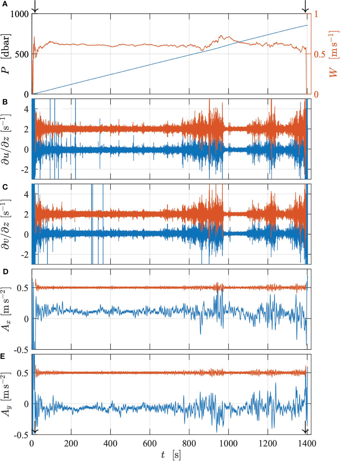
Figure 8 Time series of (A) pressure P (blue) and profiling speed W (red). (B) Original ∂u/∂z (blue) and high-pass filtered and de-spiked (red). (C) Same for ∂v/∂z. (D) Original acceleration Ax (blue) and high-pass filtered (red). (E) Same for Ay. Az is not shown. De-spiked and filtered records are offset by 2s−1 for shear and by 0.5m s−2 for accelerations. Arrows in panels (A, E) mark the start and end of the selected section.
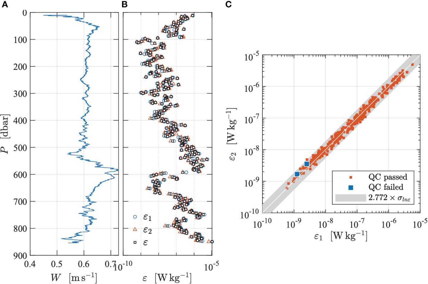
Figure 9 Dissipation estimates from the section of the time series shown in Figure 8. (A) profiling speed,W, (B) dissipation estimates from probe 1 (blue circles) and 2 (red triangles), and the average of the estimates that passed QC (black squares). (C) Scatter plot of ε1 against ε2 for estimates that passed QC (red) and those that failed (blue). Gray band is the statistical uncertainty bounded by a factor of exp(2.77 × σln ε). The uncertainty of each ε estimate is determined by its actual σln ε value, which ranges from 0.14 to 0.33 and averages to 0.23.
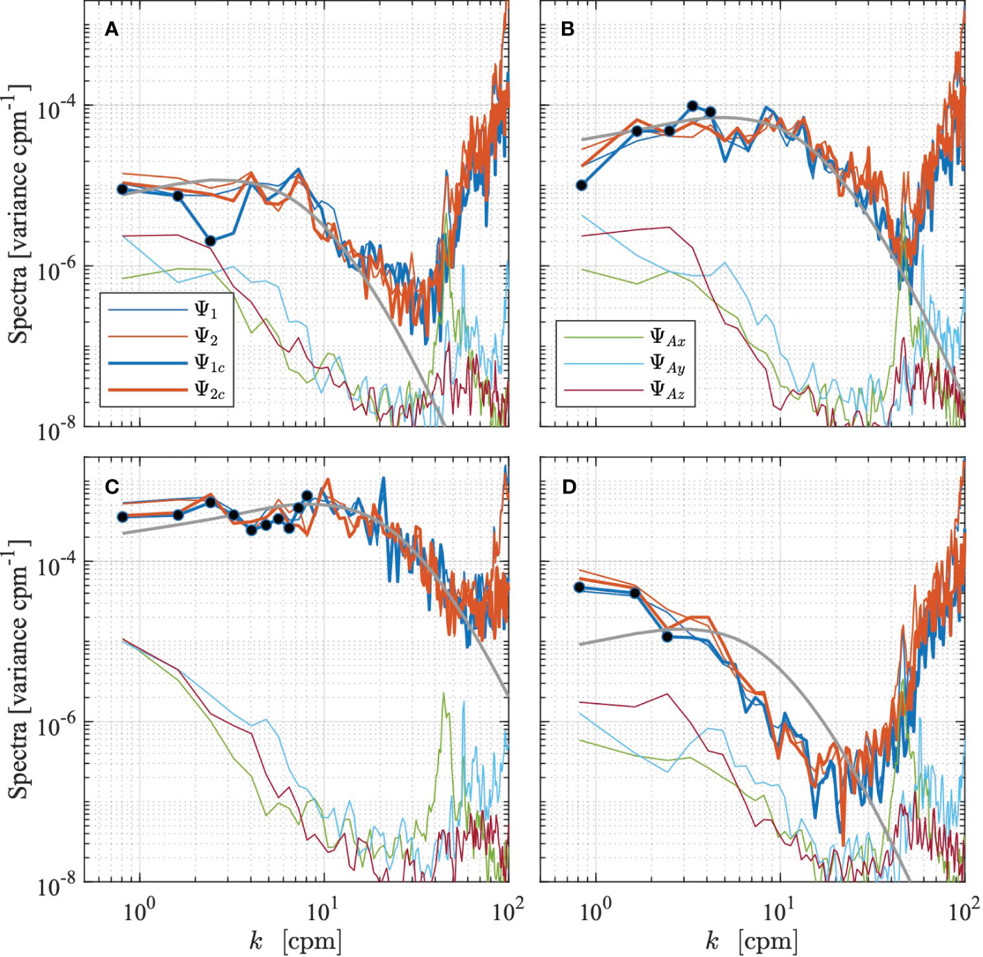
Figure 10 Wavenumber spectra from selected records (see Table 3). Wavenumbers are restricted to 100cpm. Spectra are the measured (thin) and cleaned (thick) ones of shear probe 1 (blue) and 2 (red), acceleration (green, cyan, and magenta), and the spectrum of Lueck (2022a) (gray). Panels (A–C) are low, moderate and energetic turbulence, with both probes passing QC. The spectra in panel (D) fail the QC (FOM test) for both probes. Black dots are the spectral points within the inertial subrange used for alternative estimates using fitting within the inertial subrange.
When preparing the L2 time series, the shear probe and accelerometer time series are high-pass filtered using a cutoff frequency of 0.25 Hz, which corresponds to one-half of the inverse of the FFT length (Equation 13) that is used for the analysis in L3. The shear data are cleaned, following the method of Sec. 3.2.2, using a first-order, low-pass, Butterworth filter with a cutoff frequency of 0.5 Hz and a threshold of 8. The fall rate, W is calculated from the rate of change of pressure and smoothed with a low-pass filter with a cut-off frequency of 0.5 Hz that was applied both forwards and backwards. A section is extracted from the record when W was larger than 0.4m s−1 (80% of estimated minimum fall rate) and when the depth exceeded 10m to avoid ship effects. At the typical fall rate, high-pass filtering applied in L2 will suppress the signals at vertical scales larger than the profiler length of about 2 m. Shear spectra are estimated using record lengths of 8 s and FFT lengths of 2 s that are cosine windowed and overlapped by 50%, resulting in Nf = 7. Vibration-coherent noise is removed using the records from all three accelerometers (NV = 3) with the method of Goodman et al. (2006), as described in Sec. 3.3.4. The frequency spectra are converted to wavenumber spectra using the average fall rate for each spectrum. The rate of dissipation is estimated by spectral integration (Sec. 3.4.1). Successive dissipation estimates are overlapped by 50% (i.e., about 2.4m vertical resolution using 8 s record length at 0.6m s−1).
Time series of selected parameters are shown in Figure 8 for the entire record. Early in the record, the profiler accelerates to its free fall velocity, which is approximately 0.6m s−1, and stops falling after about 1400 s when the cable is taut (Figure 8A, red). The section chosen for analysis is approximately between 10 s and 1400 s, marked by arrows. Note that only the extracted section is de-spiked and prepared for spectral analysis. Near about 600 dbar (t ≈ 875 s), a strong overturning eddy above the turbulent dense bottom current slows the profiler. This is followed by a downdraft that accelerates the profiler. Shear probe (Figures 8B, C) and horizontal acceleration (Figures 8D, E) records from L1 are shown in blue and the corresponding records of L2 that are high-pass filtered and de-spiked in red, with offset. We see that short, spiky segments of shear (Figures 8B, C, blue) are successfully removed in L2 (red). The shear axes are restricted and some outliers reach much larger values. Relatively low-frequency signals in the accelerometer records of L1 (Figures 8D, E, blue) are at vertical scales comparable to and larger than the instrument length and are filtered out in L2 (red).
Dissipation estimates from both probes agree within their expected statistical uncertainty (Equation 23), and their values span a range of 4 factors of 10 (Figure 9B). All estimates are smaller than 1 × 10⁻⁵ W kg−1 and, therefore, they were obtained using the spectral integration method. Most estimates are of high quality and pass the quality control (QC) tests (Figure 9C). Those that fail do so because they exceed the FOM criterion (the threshold was set to 1.15 in Equation 22). The final dissipation estimate is typically the average of the estimates from both probes. When the estimate from one of the probes fails the QC tests, the final estimate comes from the other probe. When both probes fail the QC test, which occurred twice, once near 100 and also near 600 dbar, no value is reported for that depth (time) range.
We select example spectra, that have been corrected for spatial probe response (Sec. 3.3.2) and high-pass filtering (Sec. 3.3.3), from three segments with low, moderate, and high dissipation rates (Figures 10A–C, respectively), all of which pass the QC (Sec. 3.4.5), and another segment when both probes fail (Figure 10D). The three sets of spectra that pass the QC show a well-defined minimum at wavenumbers ranging from 30 to 60 cpm for low and high dissipation rates, respectively. At higher wavenumbers the spectra rise because they are dominated by electronic noise. The average pressure, estimated dissipation rates and FOM for the spectra are listed in Table 3.
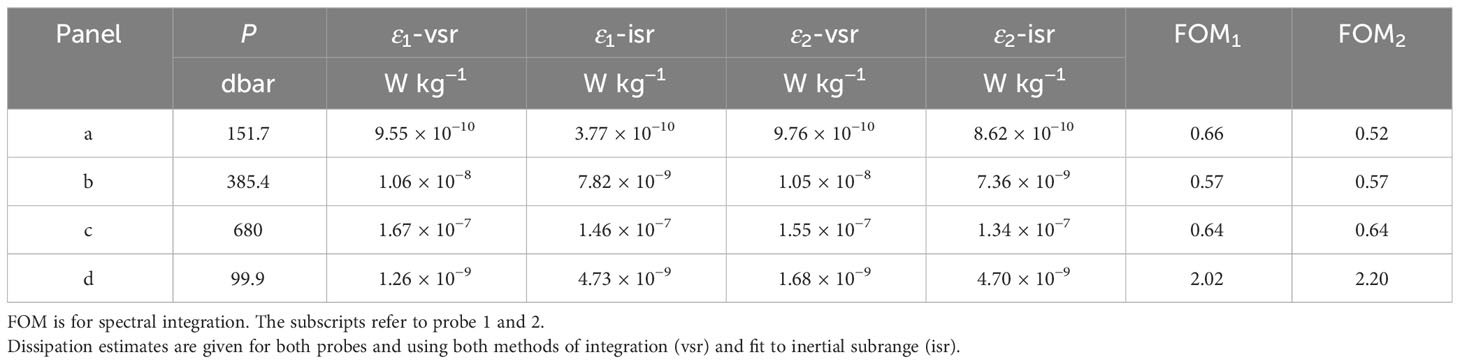
Table 3 Information about the selected spectra shown in Figure 10.
For a demonstration, we also estimated the rate of dissipation using a fitting of the spectra in the inertial subrange (Sec.3.4.2), even though this is not recommended because all rates are smaller than 10−5 W kg−1. Resulting estimates are listed in Table 3 together with the estimates from the integration method in the viscous subrange. For the quiescent spectrum (ε ≈ 1 × 10⁻⁹ W kg−1, Figure 10A), only 3 spectral points are within the inertial subrange of k ≤ 0.01(ε/ν3)1/4 (actually only 2, because our software forces inertial subrange estimates to use at least 3 points). Comparing the three marked spectra points (Figure 10A) against the reference spectrum (grey) shows that an estimate using the inertial subrange would produce a large underestimate for probe 1 (thick blue) but provide a reasonable estimate for probe 2 (thick red). For such low rates of dissipation, the estimates using the inertial subrange are unreliable because they use very little spectral information. For energetic spectra, the inertial subrange contains many points, and an estimate of ε by fitting in this range produces more reliable estimates compared to estimates for low dissipation rates. For example, ten spectral points fall within the inertial subrange in (Figure 10C) (ε = 1.5 × 10⁻⁷ W kg−1). Comparing the level of these points to the reference spectrum (gray) indicates that the inertial subrange estimates from both probes will agree closely with the estimates obtained by spectral integration. Thus, we recommend using the inertial subrange method only when dissipation rates are high, ε ≳ 10−5 W kg−1, because for lower rates spectral integration will always use more bandwidth and provide better statistical reliability.
4.2 Example of poor data
Many things can go wrong while collecting turbulence data with shear probes. The nonuniform speed of profiling is a common occurrence that can severely compromise the quality of the data reported by the shear probe. Tethered instruments must be attached to a line that is paid out rapidly enough to continuously maintain slack so that the profiler is decoupled from the motions of the deployment platform and descends smoothly throughout its profile. Sometimes, the loose tether snags, and the smooth profiling is interrupted.
The profile shown in Figure 11 was collected with a VMP-250 (manufactured by Rockland Scientific) that was deployed from a small dive-boat in the Agulhas Current about 1 km offshore from Sodwana Bay, South Africa, where the current speed exceeded 1m s−1. The target speed of the profiler was nearly double its customary value to reduce the drift of the instrument away from the boat, and to reduce the angle of attack on the shear probes due to the anticipated large rates of dissipation. Pairs of profiles were collected at each station. The fall rate of the instrument was nominal during its first profile (Figure 11A, blue), but the tether snagged on dive gear during the second profile (red). The profiler slowed its descent near 55, 193, 229, and 248 dbar. The middle two of these four interruptions jerked the profiler significantly (Figure 11C, red), which also induced a large anomaly in the shear-probe signals (Figure 11D, red). In fact, the jerk was so large that it drove the sampler of the vibration sensor into negative saturation (−215). (The vibration sensors are not calibrated and their signals are not converted into physical units because this is not necessary). Thus, even if problems with the deployment of the tether do not cause a profiler to stop descending, there can still be considerable contamination of the shear-probe signals.
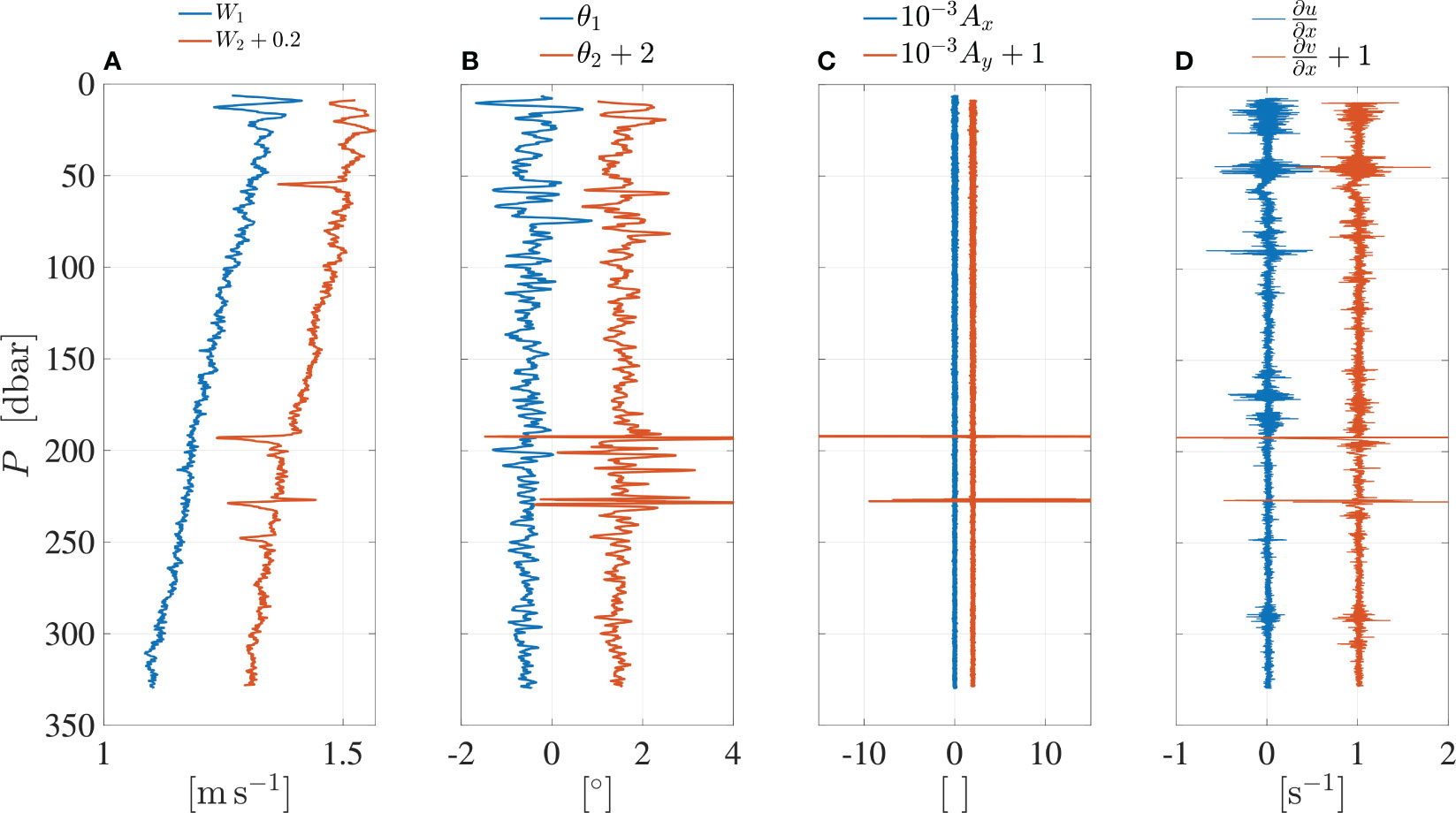
Figure 11 Two successive vertical profiles where the first (blue) was successful and the second (red) had a tether deployment problem. (A) The fall rate with four abrupt momentary decreases during the second profile. (B) The tilt of the profiler, (C) its vibrations and (D) the shear were all anomalously large near to 193 and 229dbar.
Shear spectra were computed for the second profile using data lengths of 5 s and FFT lengths of 0.5 s, that were cosine tapered and overlapped by 50%. Both vibration sensors were used to remove vibration-coherent noise from the shear-probe spectra. From Equation 17, the standard deviation of the logarithm of the spectral values is
where Nf = 19 is the number of FFT segments used for the estimate and NV = 2 is the number of vibration signals that were used to remove vibration-coherent noise. Using Equation 18, the 95% confidence interval for the spectral values is:
Spectra from a depth range free of fall-rate anomalies follow the model spectrum quite well (Figure 12A). The expected spectrum (gray) is well centered on the 95% confidence intervals of the spectra (blue and red shading). However, for both shear probes, their spectra for the region near to 193 dbar depart far from their expectation (Figure 12B). Their FOM is much larger than one and more than 5% of the data for these spectra have been modified by the de-spiking routine. The estimated dissipation rates must be rejected both because of the poor quality of the spectra (FOM ≫ 1) and because of the larger fraction of the data that was modified by the de-spiking routine (≳ 5%).
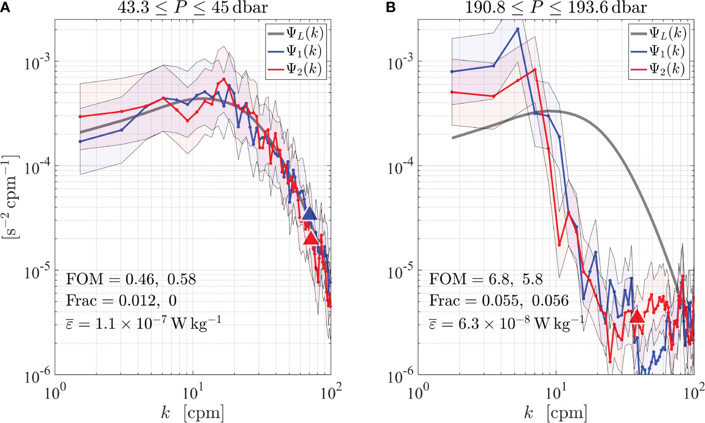
Figure 12 Spectra for the second profile shown in Figure 11 for (A) the depth range without an anomalous fall-rate and (B) for the range of the anomaly near to 193 dbar. The spectra from probes 1 (∂u/∂z) and 2 (∂v/∂z) are blue and red, respectively, while the model spectrum after Lueck (2022a) is gray. The figure of merit (FOM), the fraction of data that was altered by the de-spiking routine (Frac), and the two-probe average rate of dissipation, , are indicated within the figures. The wavenumber is restricted to 100cpm. The triangles mark the upper wavenumber limit of spectral integration. The blue and red shading provide the 95% confidence intervals for Ψ1 and Ψ2, respectively.
A de-spiking routine can often effectively remove shear anomalies due to collisions with zooplankton. However, a strong jerking of the profiler by its tether is only partially ameliorated (Figure 13 blue versus red). Similar results were obtained for the de-spiking of shear probe 2. The anomalies are reduced but the data are still not usable.
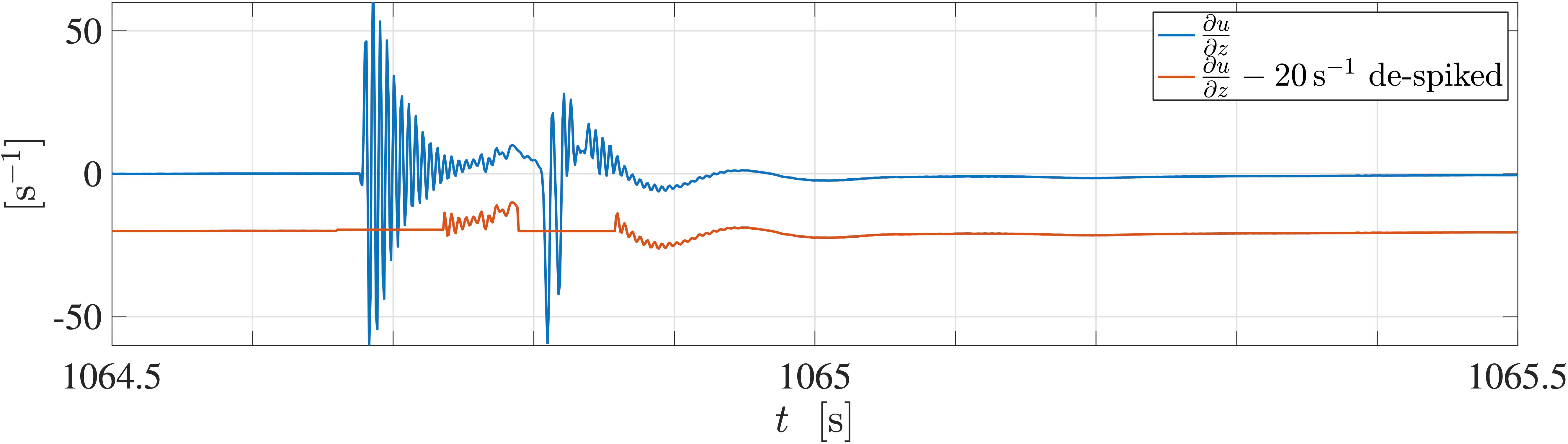
Figure 13 A close view of the original signal from shear probe 1 on the second section (profile) near to 193 dbar (blue) and this signal after it was de-spiked (red). De-spiking does not remove all anomalies and this portion of data is not suited to further processing.
5 Discussion
The ATOMIX approach described here consolidates knowledge of methods of estimating ε from shear-probe turbulence measurements while developing best practices and quality-assurance metrics for determining ε. From the outset, the Working Group sought to produce recommendations that are applicable to a range of commonly deployed platforms. This was achieved by gathering researchers from different sub-fields which brought together different experiences in terms of application and scale.
As the best practices and quality-assurance metrics were developed, it became apparent that the scientific questions and scales for the particular study are key considerations for processing. Most of the flexibility in processing choices is in L3 of the workflow. We strongly recommend the L1 and L2 steps described above. Our recommended procedure for removing spikes from shear-probe data performs well in typical conditions and is routinely used by most of the ATOMIX shear-probe group. There are different methodologies for de-spiking high-frequency resolution data, such as shear-probe signals, and an experienced user can assess whether an alternative method (e.g., using de-spiking based on nonlinear filtering) performs better for a particular dataset. In any case, we strongly recommend that the effect of de-spiking, such as the number of de-spiking passes applied, the fraction of the time series altered, etc., be documented as quality control parameters.
Two of the major choices in the workflow that are directly connected to particular scientific questions are the choices of data length for a dissipation estimate, lε, and the length of the FFT segments, lfft for a dissipation estimate. In some applications such as boundary layer profiling or thermocline studies, there will be a natural desire to use short data lengths for dissipation estimation in order to maximize the spatial resolution of the estimates. In these situations, we advise caution because shortening lε reduces the number of FFT segments in an estimated, Nf, which reduces the statistical reliability of the spectra and increases the uncertainty of the dissipation estimates. Researchers will need to evaluate and justify the trade-offs in each particular situation such as statistical reliability versus spatial resolution and the number of FFT segments.
The use of vibration-coherent noise removal is also strongly advised. Coherent noise removal increases the comparability of dissipation estimates across different platforms. Additionally, low-noise instruments may exhibit elevated shear contributions from platform vibrations in elevated turbulence regimes. An example of such data is provided in Fer et al., submitted1 (ref: VPM250 TidalChannel 24, also accessible from the ATOMIX wiki site), where shear signal contributions from platform vibrations lead to estimates of dissipation rates enhanced by more than a factor 3 in regions where dissipation rates exceed 10−5 W kg−1. We recommend the method of Goodman et al. (2006), particularly because the bias due to the statistical loss of variance inherent to the method, which may have discouraged researchers from using the method in the past, can now be corrected – Equation 16 and Ferron et al. (2023).
Clearly, the Best Practices approach can be utilised in a number of ways. For researchers and students new to the field it offers a general primer to ocean turbulence measurement using shear probes. For practitioners, it provides a synthesis of peer-developed recommendations as a shortcut to evaluate and improve their data processing. Finally, for turbulence researchers it provides a baseline from which to identify and improve gaps in the approaches. By homogenizing the data format and parameter names as described in the ATOMIX wiki and Fer et al., submitted1 we streamline both the reprocessing of the benchmark data with a user’s own routines and the inter-comparison and reproduction of scientific results.
The wider ATOMIX methodology systematically considers three different approaches to turbulence quantification in parallel developments - the other two being Acoustic Doppler Current Profiler and Acoustic Doppler Velocimetry. This consistent parallel approach provides a bridge for researchers in that they can more readily shift between techniques that best suit their application.
ATOMIX was motivated to engage with the ocean turbulence community on a number of levels. Firstly, there is a need to grow the community so that more researchers have a deeper knowledge of the measurement possibilities, limitations, and pitfalls. Secondly, any development will necessarily come from a limited set of perspectives. The advancement of the field requires a way to engage with new researchers, techniques, applications, and platforms.
One of the new applications the turbulence community is approaching relies on the integration of turbulence sensors onto autonomous platforms. Such integration already exists for platforms like ocean gliders and autonomous underwater vehicles (AUVs), but until recently, the data processing and the computation of turbulent dissipation rates were done after the deployment. This requires the platform’s recovery and limits the length of the deployments. The progress made over the last decade in microelectronics allows the development of microprocessors capable of handling the amount of data necessary to process onboard the turbulent dissipation rates (e.g., Hughes et al., 2023). The onboard processing dramatically reduces the amount of data an instrument must store to provide ε and offers the possibility of transferring turbulence data via low-bandwidth links, such as satellite communications. A platform with onboard processing and satellite communication capabilities should be able to sample the ocean over a few months or years, provided that the probes’ resilience and the battery capacity allow it.
The gain in memory space and the data compression associated with the onboard processing comes with a caveat: The quality of the data must be assessed during the processing, and quality flags accepted by the whole community should be published with the data. The present paper provides an accepted methodology and quality flags that are based on the statistical nature of turbulence measurements and are agreed upon by the ATOMIX Working Group, using three different types of microstructure sensors and different types of platforms. Such a consensus is one of the necessary steps toward global, consistent and perennial turbulence observation programs.
In a changing climate where the oceans are warming, it is vital that global ocean monitoring continues to evolve. The flagship Argo program (Roemmich et al., 1999) recently identified the observation of turbulent mixing as one of its developing branches (Roemmich et al., 2019). Building on pioneering works already integrating microstructure temperature on autonomous floats (e.g., Sherman and Davis, 1995), a handful of successful prototypes of Argo-floats equipped with microstructure sensors (shear and temperature) have already been tested, paving the way for longer deployments. A successful integration of microstructure sensors on these Argo floats would provide for the first time a systemic approach to turbulence measurement and is pushing the turbulence community to scale up the management of the turbulence data as well as the production of these sensors.
In an effort to coordinate such evolution, and largely based upon the SCOR Working Group effort presented here, the ocean mixing community is working with the Global Ocean Observing System steering committee to get the turbulent diapycnal fluxes computed from ε registered officially has an essential ocean variable (Sloyan et al., 2019). With the growing need for ocean health monitoring, the expectation is that this best practices work will be revisited, updated, and extended relatively soon.
6 Conclusions
There is an increasing availability of vehicles and platforms that can carry shear probes and a commensurate interest in exploiting them for the measurement of the rate of dissipation of turbulence kinetic energy. There is a broad spectrum of expertise among the users of shear probes that ranges from vehicle operators to scientists with a strong dedication to understanding the role of mixing in natural waters. In addition, an increasing burden is being placed on peer reviewers to judge the research that is based on shear probes. The community will benefit from guidelines and best practices for dissipation estimates, and a relatively streamlined structure of processing steps and dataset formats. The shear-probes team of the SCOR Working Group on “Analysing ocean turbulence observations to quantify mixing” (ATOMIX), aims to take the first step in consolidating knowledge and offering best practices and quality-assurance metrics for methods of estimating dissipation rates from measurements with shear probes. It is crucial to make informed choices of data processing parameters and be familiar with the limitations of the platforms, the probes, and the data processing choices that reflect on the dissipation estimates. In future studies using dissipation estimates from shear-probe data, we strongly recommend the researchers test their method and algorithm against benchmark datasets to gain confidence in their estimates. The reproducibility of dissipation estimates is only possible when the archived data have all of the required and necessary parameters together with a minimum of L1 time series records with the dissipation estimates. We highly recommend archiving data with all four levels of processing described here. Our recommendations are applicable to commonly deployed platforms and will facilitate the reproducibility of dissipation estimates and their interpretation. As ocean monitoring continues to evolve, we expect that this best practices work will be updated and extended. A desired and necessary extension is the development of such best practices for the rate of dissipation of turbulence temperature variance.
Data availability statement
Publicly available datasets were analyzed in this study. This data can be found here: NERC EDS British Oceanographic Data Centre NOC, http://doi.org/10.5285/05f21d1d-bf9c-5549-e063-6c86abc0b846.
Author contributions
RL: Conceptualization, Investigation, Methodology, Visualization, Writing – original draft, Writing – review & editing. IF: Conceptualization, Investigation, Methodology, Visualization, Writing – original draft, Writing – review & editing. CB: Methodology, Writing – review & editing. MD: Investigation, Methodology, Writing – review & editing. PH: Methodology, Software, Writing – review & editing. RI: Methodology, Writing – review & editing. AL: Investigation, Methodology, Writing – review & editing. S-AN: Methodology, Writing – review & editing. KS: Methodology, Visualization, Writing – review & editing. CS: Methodology, Visualization, Writing – review & editing.
Funding
The author(s) declare financial support was received for the research, authorship, and/or publication of this article. This manuscript is based on work conducted by the Scientific Committee on Oceanic Research (SCOR) Working Group 160: “Analysing ocean turbulence observations to quantify mixing” (ATOMIX). SCOR Working Group 160 is funded by the NSF grant to SCOR OCE-2140395 as well as by contributions from national SCOR committees.
Acknowledgments
We are grateful to the other members of the ATOMIX group and to the numerous researchers who read our initial draft and provided useful comments and suggestions, including Jeff Carpenter, Bruno Ferron, Isabelle Giddy, Sjoerd Groeskamp, Ken Hughes, Achim Randelhoff, and Elena Roget. Thoughtful and critical comments from two reviewers helped improve an earlier version of the manuscript.
Conflict of interest
Author RL is employed part time by Rockland Scientific Inc.
The remaining authors declare that the research was conducted in the absence of any commercial or financial relationships that could be construed as a potential conflict of interest.
Publisher’s note
All claims expressed in this article are solely those of the authors and do not necessarily represent those of their affiliated organizations, or those of the publisher, the editors and the reviewers. Any product that may be evaluated in this article, or claim that may be made by its manufacturer, is not guaranteed or endorsed by the publisher.
Footnotes
- ^ Fer, I., Dengler, M., Holtermann, P., Le Boyer, A., and Lueck, R. (2024). ATOMIX benchmark datasets for dissipation rate measurements using shear probes. Sci. Data. Submitted.
References
Allen H. J., Perkins E. W. (1951). A study of effects of viscosity on flow over slender inclined bodies of revolution (Report 1048, National Advisory Committee for Aeronautics).
Dataset Fer I. (2023). ATOMIX shear probes benchmark data: a dissipation profile from the Faroe Bank Channel overflow obtained by a vertical microstructure profiler in June 2012. NERC EDS British Oceanographic Data Centre NOC. doi: 10.5285/05f21d1d-bf9c-5549-e063-6c86abc0b846
Fer I., Bakhoday Paskyabi M. (2014). Autonomous ocean turbulence measurements using shear probes on a moored instrument. J. Atmos. Ocean. Technol. 31, 474–490. doi: 10.1175/JTECH-D-13-00096.1
Fer I., Peterson A. K., Ullgren J. E. (2014). Microstructure measurements from an underwater glider in the turbulent Faroe Bank Channel overflow. J. Atmospheric Oceanic Technol. 31, 1128–1150. doi: 10.1175/JTECH-D-13-00221.1
Fer I., Voet G., Seim K. S., Rudels B., Latarius K. (2010). Intense mixing of the Faroe Bank Channel overflow. Geophys. Res. Lett. 37, L02604. doi: 10.1029/2009GL041924
Ferron B., Bouruet Aubertot P., Cuypers Y., Vic C. (2023). Removing biases in oceanic turbulent kinetic energy dissipation rate estimated from microstructure shear data. J. Atmospheric Oceanic Technol. 40, 129–139. doi: 10.1175/JTECH-D-22-0035.1
Fleury M., Lueck R. G. (1992). Microstructure in and around a double-diffusive interface. J. Phys. Oceanography 22, 701–718. doi: 10.1175/1520-0485(1992)
Frajka-Williams E., Brearley J. A., Nash J. D., Whalen C. B. (2022). “Chapter 14 - New technological frontiers in ocean mixing,” in Ocean Mixing. Eds. Meredith M., Garabato A. N. (Elsevier), 345–361. doi: 10.1016/B978-0-12-821512-8.00021-9
Goodman L., Levine E. R., Lueck R. G. (2006). On measuring the terms of the turbulent kinetic energy budget from an auv. J. Atmospheric Oceanic Technol. 23, 977–990. doi: 10.1175/JTECH1889.1
Gregg M. C. (2021). Ocean Mixing (Cambridge: Cambridge University Press). doi: 10.1017/9781316795439
Hughes K. G., Moum J. N., Rudnick D. L. (2023). A turbulence data reduction scheme for autonomous and expendable profiling floats. Ocean Sci. 19, 193–207. doi: 10.5194/os-19-193-2023.
Jenkins D., Quintana-Ascencio P. (2020). A solution to minimum sample size for regression. PloS One 15, 1–15. doi: 10.1371/journal.pone.0229345.
Kolmogorov A. N. (1941). Local structure of turbulence in an incompressible fluid at very high Reynolds number. Doklady AN SSSR 4, 299–303.
Lueck R. (2022a). The statistics of ocenic turbulence measurements. Part 2: Shear spectra and a new spectral model. J. Atmospheric Oceanic Technol. 39, 1273–1282. doi: 10.1175/JTECH-D-21-0050.1
Lueck R. G. (2022b). The statistics of oceanic turbulence measurements. Part 1: Shear variance and dissipation rates. J. Atmospheric Oceanic Technol. 39, 1259–1271. doi: 10.1175/JTECH-D-21-0051.1
Lueck R. G., Huang D., Newman D., Box J. (1997). Turbulence measurement with a moored instrument. J. Atmospheric Oceanic Technol. 14, 143–161. doi: 10.1175/1520-0426(1997)014<0143:TMWAMI>2.0.CO;2
Macoun P., Lueck R. (2004). Modelling the spatial response of the airfoil shear probe using different sized probes. J. Atmospheric Oceanic Technol. 21, 284–297.
McMillan J. M., Hay A. E., Lueck R. G., Wolk F. (2016). Rates of dissipation of turbulent kinetic energy in a high reynolds number tidal channel. J. Atmospheric Oceanic Technol. 33, 817–837. doi: 10.1175/JTECH-D-15-0167.1
Moum J. N., Gregg M. C., Lien R. C., Carr M. E. (1995). Comparison of turbulence kinetic energy dissipation rate estimates from two ocean microstructure profilers. J. Atmospheric Oceanic Technol. 12, 346–366. doi: 10.1175/1520-0485(1995)025<1913:OOTMIN>2.0.CO;2
Nagai T., Inoue R., Yamazaki A. T. H. (2015). Evidence of enhanced double-diffusive convection below the main stream of the kuroshio extension. J. Geophysical Res. – Oceans 120, 8402–8421. doi: 10.1002/2015JC011288
Nasmyth P. W. (1970). Ocean turbulence. Ph.D. thesis. University of British Columbia, Vancouver, British Columbia, Canada.
Naveira Garabato A. C., Frajka-Williams E. E., Spingys C. P., Legg S., Polzin K. L., Forryan A., et al. (2019). Rapid mixing and exchange of deep-ocean waters in an abyssal boundary current. Proc. Natl. Acad. Sci. 116, 13233–13238. doi: 10.1073/pnas.1904087116
Nuttall A. (1971). Spectral estimation by means of overlapped fast fourier transform processing of windowed data (NUSC Tech. Rep. 4169, Naval Underwater Systems Center).
Oakey N. S. (1982). Determination of the rate of dissipation of turbulent kinetic energy from simultaneous temperature and velocity shear microstructure measurements. J. Phys. Oceanography 12, 256–271.
Osborn T. R. (1974). Local vertical profiling of velocity microstructure. J. Phys. Oceanography 4, 109–115.
Osborn T. R., Crawford W. R. (1980). “An airfoil probe for measuring turbulent velocity fluctuations in water,” in Air-Sea Interaction: Instruments and Methods. Eds. Dobson F. W., Davis R. (New York: Plenum), Mechanical Engineering), 535.
Osborn T. R., Farmer D. M., Vagle S., Thorpe S. A., Cure M. (1992). Measurements of bubble plumes and turbulence from a submarine. Atmosphere-Ocean 30, 419–440. doi: 10.1080/07055900.1992.9649447.
Palmer M. R., Stephenson G. R., Inall M. E., Balfour C., Duesterhus A., Green J. A. M. (2015). Turbulence and mixing by internal waves in the Celtic Sea determined from ocean glider microstructure measurements. J. Mar. Syst. 144, 57–69. doi: 10.1016/j.jmarsys.2014.11.005
Panchev S., Kesich D. (1969). Energy spectrum of isotropic turbulence at large wavenumbers. Comptes rendus lacademie Bulgare Des. Sci. 22, 627–630.
Roemmich D., Alford M. H., Claustre H., Johnson K., King B., Moum J., et al. (2019). On the future of argo: A global, full-depth, multi-disciplinary array. Front. Mar. Sci. 6, 439. doi: 10.3389/fmars.2019.00439.
Roemmich D., Boebel O., Desaubies Y., Freeland H., King B., LeTraon P.-Y., et al. (1999). Argo: The global array of profiling floats. CLIVAR Exchanges 13, 4–5.
Roget E., Lozovatsky I., Sanchez-Martin X., Figueroa M. (2006). Microstructure measurements in natural waters: Methodology and applications. Prog. Oceanography - Prog. OCEANOGR 70, 126–148. doi: 10.1016/j.pocean.2006.07.003
Sherman J. T., Davis R. E. (1995). Observations of temperature microstructure in natre. J. Phys. oceanography 25, 1913–1929. doi: 10.1175/1520-0485(1995)025<1913:OOTMIN>2.0.CO;2
Siddon T. E. (1965). A turbulence probe utilizing aerodynamic lift. Tech. Rep. 88, University of Toronto.
Siddon T. E. (1971). A miniature turbulence gauge for utilizing aerodynamic lift. Rev. Sci. Instruments 42, 653–656. doi: 10.1063/1.1685193
Sloyan B. M., Wilkin J., Hill K. L., Chidichimo M. P., Cronin M. F., Johannessen J. A., et al. (2019). Evolving the physical global ocean observing system for research and application services through international coordination. Front. Mar. Sci. 6, 449. doi: 10.3389/fmars.2019.00449.
Sreenivasan K. R. (1995). On the universality of the Kolmogorov constant. Phys. Fluids 7, 2778–2784. doi: 10.1063/1.868656
St. Laurent L. S. M. (2017). Measurements of near-surface turbulence and mixing from autonomous ocean gliders. Oceanography 30, 116–125. doi: 10.5670/oceanog.2017.231
Taylor G. (1935). Statistical theory of turbulence. Proc. R. Soc A 151, 421–444. doi: 10.1098/rspa.1935.0159
Waterhouse A. F., MacKinnon J. A., Nash J. D., Alford M. H., Kunze E., Polzin H. L. S. K. L., et al. (2014). Global patterns of diapycnal mixing from measurements of the turbulent dissipation rate. J. Phys. Oceanography 44, 1854–1872. doi: 10.1175/JPO-D-13-0104.1
Wesson J. C., Gregg M. C. (1994). Mixing at camarinal sill in the strait of Gibraltar. J. Geophysical Res. 99, 9847–9878. doi: 10.1029/94JC00256
Wolk F., Yamazaki H., Seuront L., Lueck R. G. (2002). A new free-fall profiler for measuring bio-physical microstructure. J. Atmospheric Oceanic Technol. 19, 780–793.
Keywords: turbulence, rate of dissipation, shear spectra, shear variance, shear probes
Citation: Lueck R, Fer I, Bluteau C, Dengler M, Holtermann P, Inoue R, LeBoyer A, Nicholson S-A, Schulz K and Stevens C (2024) Best practices recommendations for estimating dissipation rates from shear probes. Front. Mar. Sci. 11:1334327. doi: 10.3389/fmars.2024.1334327
Received: 07 November 2023; Accepted: 31 January 2024;
Published: 19 March 2024.
Edited by:
Jay S. Pearlman, Institute of Electrical and Electronics Engineers, FranceReviewed by:
John Toole, Woods Hole Oceanographic Institution, United StatesLou St Laurent, University of Washington, United States
Copyright © 2024 Lueck, Fer, Bluteau, Dengler, Holtermann, Inoue, LeBoyer, Nicholson, Schulz and Stevens. This is an open-access article distributed under the terms of the Creative Commons Attribution License (CC BY). The use, distribution or reproduction in other forums is permitted, provided the original author(s) and the copyright owner(s) are credited and that the original publication in this journal is cited, in accordance with accepted academic practice. No use, distribution or reproduction is permitted which does not comply with these terms.
*Correspondence: Rolf Lueck, rolf@rocklandscientific.com