Recent large-scale mixed layer and vertical stratification maxima changes

1 Introduction

The intensity of upper-ocean stratification has profound impact on the climatic system as it modifies or shapes physical mechanisms at work and the marine ecosystem. The vertical transfer of heat, matter and momentum in the ocean, including ventilation, upwelling and entrainment into the mixed layer are affected by the density distribution below the mixed layer and therefore depend on the stratification (Capotondi et al., 2012; Cronin et al., 2013). Mixed layer dynamics impact air-sea exchange of carbon (Bopp et al., 2015) and influence deoxygenation processes in the subtropical-tropical oceans (Schmidtko et al., 2017; Oschlies et al., 2018). Upwelling and mixing in turn play a key role for the nutrient supply to the euphotic zone which further influences phytoplankton abundance and fisheries (e.g., Fiedler et al., 2013; Llort et al., 2019). Additionally, upper-ocean stratification changes play a role in upper-ocean heat content and air-sea interactions which in turn can influence phenomena such as tropical storms or rainfall (Balaguru et al., 2016).

This study aims to address recent changes of the vertical stratification maximum and mixed layer properties from Argo observations for the time period of 2006-2021 (Argo, 2021). Due to its tight relation to the mixed layer, the vertical stratification maximum is a gateway for ocean ventilation and nutrient supply to the euphotic zone.

The upper-ocean can be described by three layers: the surface mixed layer, the seasonal and permanent pycnocline (Sprintall and Cronin, 2009). Additionally, a transient layer located directly below the surface mixed layer is often employed to describe exchange processes between the mixed layer and the ocean interior (Ferrari and Boccaletti, 2004; Johnston and Rudnick, 2009). It is sometimes part of the seasonal pycnocline. The surface mixed layer is characterized by well-mixed hydrographic properties and undergoes a seasonal cycle, being typically deeper in winter and shallower in summer. The mixed layer properties are subject to atmospheric forcings, such as wind, heat and freshwater (Sprintall and Cronin, 2009). These forcings lead to mixed layer variations on all timescales and result in a mean latitudinal mixed layer depth distribution, being deep at high latitudes and shallow in the tropical oceans (Sprintall and Cronin, 2009).

Below the mixed layer, density increases strongly with depth, creating local maxima in the vertical density gradient (Sprintall and Cronin, 2009). This transition layer is characterized by high vertical shear and connects the highly turbulent surface mixed layer with the weakly turbulent ocean interior (Ferrari and Boccaletti, 2004; Johnston and Rudnick, 2009; Kaminski et al., 2021). During summer, the seasonal pycnocline is within the transient layer. The seasonal pycnocline forms during spring from detrainment of the shoaling mixed layer and entrains its waters back into the deepening winter mixed layer. It is the midterm memory of the upper-ocean by which summer conditions impact the start and/or strength of winter processes (Sprintall and Cronin, 2009; Huang, 2010). Below, there exists the permanent pycnocline. Owing to the seasonal cycle of the mixed layer, the permanent pycnocline develops from late-winter properties of the deep winter mixed layer only: when isopycnal outcrops are closest to the equator and the mixed layers are deepest in late winter, there is a time frame of 1-2 months, where water from the mixed layer reaches the permanent pycnocline (Williams and Meijers, 2019). The permanent pycnocline separates the upper from the deep ocean on an all-year basis (Iselin, 1939; Stommel, 1979; Williams et al., 1995; Sprintall and Cronin, 2009; Huang, 2010; Feucher et al., 2019). Note, subduction is a non-local process, i.e., since the water, detrained from the mixed layer, is moving downstream by currents. Hence, the late winter properties found in the permanent pycnocline originate from a different location as where they are subducted (Huang, 2010).

However, not in all areas of the world oceans these types of seasonal and permanent pycnoclines are present, e.g., in the high polar regions no permanent pycnocline exists (Sprintall and Cronin, 2009). In the tropical ocean a shallow pycnocline (thermocline) exists in all seasons since there is only a weak seasonal cycle of the mixed layer depth. Towards the subtropics and high latitudes, the seasonality increases and thus induces the above discussed seasonal pycnocline above the permanent pycnocline (e.g., Wyrtki, 1964; Fiedler and Talley, 2006). Thus, a separation into seasonal and permanent pycnoclines is not always possible.

The maximum vertical density gradient can be detected via the Brunt-Väisälä frequency as the vertical stratification maximum which has an influence on e.g., buoyancy and heat budgets, but also plays a role for oxygen and nutrient distributions (Fiedler et al., 2013). Regionally and seasonally, the vertical stratification maximum can have a severely different meaning in the water column, as it may locally be the transition from the mixed layer to the seasonal or permanent pycnocline, or e.g., in summer be part of the seasonal pycnocline itself.

Climate models project an intensifying stratification, accompanied by mixed layer shoaling. This is associated with a reduced ocean ventilation under the global warming scenario (e.g., Keeling et al., 2010; Capotondi et al., 2012; Rhein et al., 2013; Kwiatkowski et al., 2020). Consequences of strengthened stratification and poleward movement of outcropping areas of isopycnals due to subtropical ocean surface warming are suggested to lead to a shallowing of subducted ventilated layers and an oxygen loss below the tropical thermocline (Oschlies et al., 2018). Furthermore, assuming thinner mixed layers, lateral induction, an important process in the mode water formation, could decline (Oschlies et al., 2018).

Observational evidence suggests that these relationships are ambiguous and the causes of stratification changes in a warming world are not yet fully understood. Despite ocean surface warming, stratification does not strengthen everywhere (Somavilla et al., 2017). Large-scale mixed layer deepening is counterintuitive to enhanced stratification owing to changes in buoyancy forcings and wind-driven Ekman pumping (Somavilla et al., 2017). Observations indicate summertime mixed layer deepening accompanied by enhanced stratification below the mixed layer base (Sallée et al., 2021). Two methodically-different studies show stratification has been increasing since the 1960s (Yamaguchi and Suga, 2019; Li et al., 2020): Stratification has been rising by 3.3-6.1% in the upper 200 m and it has been intensifying in 40% of the global oceans (Yamaguchi and Suga, 2019). The upper 2000 m of the water column are experiencing an enhanced stratification of 5.3% with greatest increase in the upper 150 m (5-18%) (Li et al., 2020). All above studies investigated stratification over a large depth range or at the base of the mixed layer. Despite both methods reveal an increase of stratification in the various parts of the water column, they have specific advantages and limitations. All stratification analyses that average over a depth range have to deal with a loss of the vertical density structure and thus, limit the understanding of the processes at play. The pycnocline locations and mixed layer depths vary globally, hence such a method regionally misses profound stratification maxima changes wherever the mixed layer is deeper or much shallower than the evaluated depth range (Sallée et al., 2021). Nevertheless, an advantage of a depth-range-averaged stratification measure is its ability to relate it to ocean heat content variations in the same depth range.

This investigation concentrates on the vertical stratification maximum which is defined as a local pycnocline and is thought to play a key role for the exchange between the mixed layer and the interior ocean as well as for how deep the mixed layer can reach. Our method frames the true maximum of the vertical stratification of the local water column which does not have to be the first local maximum below the mixed layer as studied recently by Sérazin et al. (2023). Indeed, the vertical stratification maximum location is highly variable among regions and summer and winter season. Therefore, it cannot be assigned to a specific layer for the global ocean. It depends on the region, in which upper-ocean layer the vertical stratification maximum is located. In general, it can be part of the transition layer when the maximum is found just below the mixed layer and its magnitude is comparable to the one in the transition layer. But in regions, where the stratification maximum is much deeper than the mixed layer and larger in magnitude than the transition layer stratification, it is hardly determining the transition layer. Here, we do not aim for a layer thickness, yet we focus on the location and magnitude of the vertical stratification maximum for its simplicity of determining this variable.

The vertical stratification maximum is a part of the ocean that has not yet been investigated in detail. In contrast to seasonal and permanent pycnoclines, it is a variable which is well-defined in all areas of the ocean and related to exchange processes between the surface mixed layer and ocean interior. The vertical stratification maximum is located at a depth that can be easily determined and is therefore a parameter that is well-comparable to models. It is not subject to the high variability as found for the base of the mixed layer. Making excessive use of the vast amount of Argo observations (Argo, 2021), we map summer and winter vertical stratification maxima. This dataset represents the mean state of the vertical stratification maxima in the past 16 years and gives detailed insights about the variability of the summer and winter stratification maxima on multi-year time scales. The last decade (2010-2019) is of especially large interest since the ocean surface warming has intensified by 0.280 ± 0.068°C decade^-1 compared to the warming rate of 0.062 ± 0.013°C decade^-1 of the last 120 years (1900-2019) (Garcia-Soto et al., 2021). With the Argo observations we are able to investigate the decade of accelerated warming in more detail and explore regional differences in stratification and mixed layer changes as well as their possible causes. It is not possible to directly link the observed changes of stratification and mixed layer characteristics to climate warming as a short time period of 16 years is subject to natural climate variability, too. We aim to provide a data product of an upper-ocean variable that can be easily compared to model and reanalysis outputs for validation and process analysis.

2 Data and methods

2.1 Argo observations

As hydrographic dataset we use Argo observations from 2006-2021 (Argo, 2021). The Argo floats are profiling the upper 2000 m and since 2006 the Argo coverage has overcome larger gaps and it allows for global analyses (Roemmich et al., 2015; Desbruyères et al., 2017). Here, we use profiles that are identified as good data by the quality control procedures (QC=1), taking only those from the adjusted data mode into account. Additional quality controls applied are the following: pressure profiles have to be continuous and reach at least 1000 dbar, vertical profiles may not have a pressure difference between two adjacent pressure points larger than 150 dbar and more than 20 sample points have to be present in the upper 2000 dbar. Globally, 1,559,383 profiles pass this quality check. Temporal and spatial distributions of the Argo profiles have been checked (Supplementary Figure S1). Some regions as the central subtropical South Pacific and south of 60°S should be evaluated with more caution as the number of profiles and maximum time span is observed to be reduced (Supplementary Figure S1). Conversion of in situ measurements into absolute salinity, conservative temperature and potential density is done using TEOS-10 (McDougall and Barker, 2011). Note that the vertical resolution of an individual Argo profile is usually not distributed uniformly over the water column, but generally has a higher resolution in the upper 500 dbar. The median pressure difference between two adjacent pressure measurements in the upper 500 dbar of all profiles is 5-6 dbar. Since in most regions the vertical stratification maximum is confined to the upper 500 dbar of the ocean, it is well-detected by most profiles.

For each profile mixed layer depth, temperature and salinity are estimated by the Holte and Talley algorithm (Holte and Talley, 2009) which evaluates the mixed layer characteristics by a combination of threshold and gradient (Holte and Talley, 2009).

2.1.1 Argo profile treatment and stratification estimate

Vertical resolution among Argo profiles varies. Particularly, the newer Iridium floats contain a higher vertical sampling rate than the older ARGOS floats. In order to overcome this irregularity of vertical sampling, we interpolate all profiles on an isopycnal grid prior to our analysis of the vertical stratification maxima. We chose the isopycnal interpolation for this study as it maintains the vertical stratification (Schmidtko et al., 2013) and hence, this formulation mitigates possible errors of the vertical stratification maximum. Statistical comparison shows that isopycnal gridding on average performs better than isobaric gridding (Supplementary Figure S2). This is due to the non-linearity of the equation of state for seawater which is accounted for by the isopycnal gridding performed in theta-salinity space, but not by the isobaric gridding.

For the measure of stratification, we choose the square of the Brunt-Väisälä frequency, N², following the definition in TEOS-10 (IOC et al., 2010; McDougall and Barker, 2011):

where g is the gravitational acceleration, ρ is the potential density, α and β refer to the thermal expansion and saline contraction coefficients, respectively. dT and dS_A are differences in conservative temperature and absolute salinity over a pressure difference dP (IOC et al., 2010). This function, implemented in the Gibbs SeaWater (GSW) Oceanographic Toolbox of the International Thermodynamic Equation of State – 2010 (IOC et al., 2010) originates from the definition by Gill (Gill, 1982) (cf. his equation 3.7.9). This way of calculating the Brunt-Väisälä frequency is proposed to be the desired one when conservative temperature and absolute salinity profiles are interpolated or fitted beforehand which is the case for our study (McDougall and Barker, 2014).

In the following we provide a step-by-step guide on our interpolation scheme and the determination of the vertical stratification maximum.

Step 1: The profiles of conservative temperature, absolute salinity and pressure are interpolated on an isopycnal grid. This grid consists of 433 levels ranging from 20.0 kg m^-3 to 29.5 kg m^-3. The isopycnal grid is assigned into several subsets of different intervals between isopycnals with increasing resolution for higher density levels. Lower density levels (20.0 kg m^-3 -23.95 kg m^-3) have a grid space difference of 0.12 kg m^-3. This grid interval becomes smaller over several subsets down to 0.005 kg m^-3 for isopycnal levels larger than 28.15 kg m^-3. This isopycnal grid has been chosen in order to be able to resolve the vertical structure in subpolar regions and the Mediterranean Sea. These regions contain much higher density values from surface to bottom and to assure a reasonable grid spacing, the isopycnal intervals are decreasing for higher isopycnal levels. The isopycnal levels and intervals are chosen by the compromise of taking the computational efficiency and a sufficiently well-resolved upper-ocean into account.

For the interpolation we applied the modified Akima piecewise cubic Hermite interpolation [makima method (MathWorks Inc., 2019; MATLAB, 2019)] which is based on the algorithm from Akima (Akima, 1970) and combines the interpolation schemes of cubic spline and the piecewise cubic Hermite interpolating polynomial (pchip) (MathWorks Inc., 2019). To determine vertical maxima and minima from an individual profile, an interpolation scheme is required which allows for local maxima and minima between measurements (Roch et al., 2021). The makima method enables undulations in contrast to the pchip method and at the same time prevents artificial spline maxima between identical samples.

Step 2: Some profiles cover only part of the density range due to outcropping isopycnals. This is handled mathematically by using mixed layer properties above the surface for ease of computational analysis. Note that on an isopycnal grid the mixed layer does not need any other grid points than at the mixed layer base and at the surface since the density in the mixed layer is the same at all depth levels (Figures 1A–C).

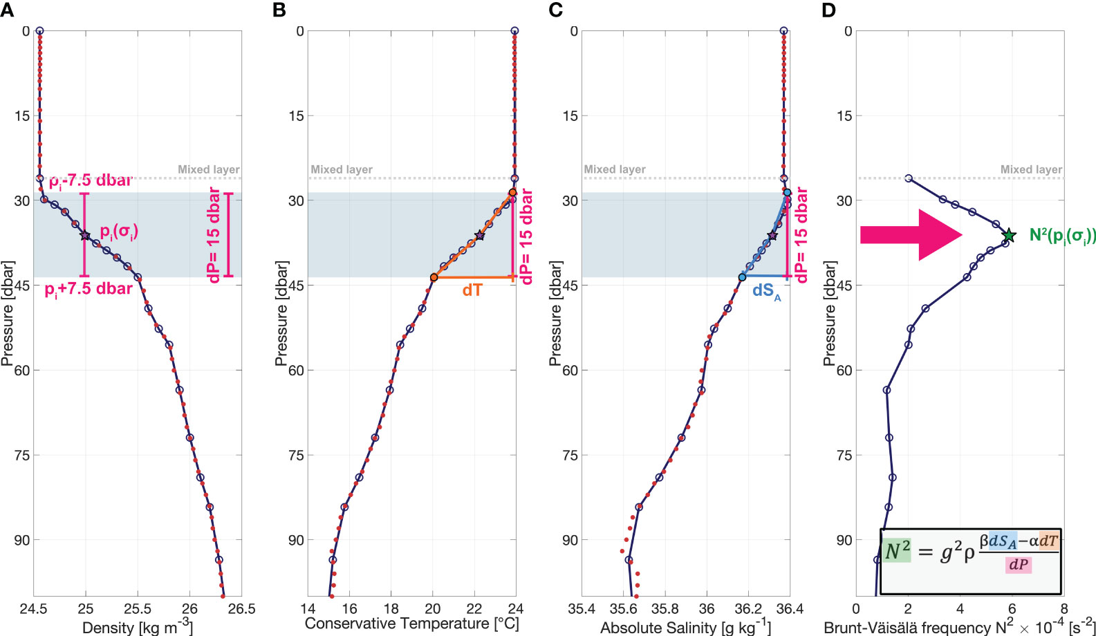
Figure 1 Density-interpolated Argo profile. Snapshot of an example Argo profile after applying density-interpolation for (A) pressure, (B) conservative temperature, (C) absolute salinity and (D) the therefrom resultant squared Brunt-Väisälä frequency profile. The blue lines with bullets show the profiles received after makima interpolation method on the isopycnal grid. The bullets denote the chosen isopycnal grid and red dots refer to the un-interpolated measurement points of the Argo profile. Additionally, the mixed layer is indicated by the grey dotted line. The light blue shaded bar as well as the pink vertical lines in (A–C) indicate the dP=15-dbar window chosen for the computation of the Brunt-Väisälä frequency. The density-interpolated pressure grid point p_i(σ_i) is found at the center of these bars and marked by a purple star (A–C). Due to the 15-dbar window, we achieve three different points: p_i(σ_i) and p_i ± 7.5 dbar. As indicated by the orange lines in (B) for temperature and by the blue lines in (C) for salinity, it is linearly interpolated among the corresponding three points. From this three-point interpolation, dT [horizontal orange line in (B)] and dS_A [horizontal blue line in (C)] can be computed for each corresponding dP=15-dbar window. Following the equation for the Brunt-Väisälä frequency in (D), the resulting Brunt-Väisälä frequency profile is achieved. The green star in (D) corresponds to the grid point indicated by the purple stars in (A–C).

Step 3: For the calculation of the Brunt-Väisälä frequency, we set dP = 15 dbar in Eq. 1. We choose the constant window size of 15-dbar instead of the layer thickness between isopycnals, in order to maintain a comparable parameter and to avoid troubleshooting with globally varying isopycnal depths and layer thicknesses. The constant window size is applied to each isopycnal grid point σ_i (i referring to the isopycnal level).

The pressure at each isopycnal grid point, p_i(σ_i), is the midway pressure point to which the final estimate of N² will be referenced. Then, the corresponding upper and lower limits of the 15-dbar window are defined as follows: [p_i(σ_i) - 7.5 dbar, p_i(σ_i) + 7.5 dbar] (Figure 1A). Together with the midway pressure point p_i(σ_i) this results in three vertical points.

Step 4: To determine the salinity and temperature values for the upper and lower limits of the 15-dbar window, linear interpolation between the nearest grid points of the isopycnal grid is applied. The difference between the determined values at the upper and lower limits provides dT (horizontal orange bar in Figure 1B) and dS_A (horizontal blue bar in Figure 1C) corresponding to dP = 15 dbar (Figures 1A–C by the vertical pink bar). dT and dS_A are individual for each isopycnal grid point σ_i.

Step 5: dT, dS_A and dP = 15 dbar are then inserted into Eq. 1. From Eq. 1 the square of the Brunt-Väisälä frequency, N², is obtained as a function of the isopycnal grid and the corresponding pressure p_i(σ_i) (Figure 1D). This procedure provides Brunt-Väisälä frequency profiles that are vertically smoothed as a result of the 15-dbar window. This filter allows for a good representation of local maxima and minima of the vertical profiles but reduces small-scale noise and variability which would become dominant for smaller vertical windows.

Step 6: Finally, the vertical stratification maximum and its depth are derived from each Brunt-Väisälä frequency profile as the maximum value and the depth of the corresponding isopycnal grid point.

This method does yield different results compared to taking stratification directly below the mixed layer (Sallée et al., 2021) into account as for 73% of the Argo profiles the vertical stratification maximum is found deeper than within the 15 m layer below the mixed layer base. Additionally, our method estimates stratification on an isopycnal grid which is in contrast to all above-noted methodically-different studies. Isopycnal gridding benefits over isobaric gridding as it does not create artificial water masses, but maintains water mass properties and the vertical stratification (Lozier et al., 1994; Schmidtko et al., 2013). Since averaging errors are significantly reduced when using isopycnal instead of isobaric schemes, Lozier et al. (1994) proposed the use of potential density surfaces for creating hydrographic climatologies.

Note, for the isopycnal heave analysis, isopycnal coordinates are converted to depth coordinates. This is done via linear interpolation on an even depth grid with a 5m-stepwidth from the sea surface to 1000 m. A transformation to depth surfaces is necessary, in order to compare the isopycnal displacements to the mixed layer depth and pycnocline depth changes during the zonal analyses.

Since the density distributions vary among the Atlantic, Pacific and Indian Oceans, we applied the zonal heave analysis for each ocean separately. We exclude the Mediterranean Sea from the calculation for the Atlantic Ocean as it has much higher density than the rest of the subtropical North Atlantic.

2.1.2 Mapping processes and trend calculations

Mapping of the individual parameters (vertical stratification maximum, its depth, mixed layer temperature, salinity and depth) is done on a 1° x 1° grid in latitude and longitude. For each grid point data within an ellipse is taken into account. To preserve the more zonal structures in low latitudes, along the equator 6° radius in latitude and 14° radius in longitude is the maximum distance of used data. The elliptic radii gradually change toward circle radii at 20°N/S following an exponential function, while preserving the spatial area of the ellipses and circles. For each grid point and parameter to be mapped an interquartile range (IQR) filter is used, excluding data outside 1.5 times the IQR above the third quartile or 1.5 times the IQR below the first quartile. This is equivalent to a 99.3% standard deviation filter on a normal distribution.

In order to account for the different distances of the profiles to the grid points, we include a distance weighting function in the mapping process (Schmidtko et al., 2013):

Where Δd is the distance between each profile location and the corresponding grid point i, and L is the spatial decorrelation scale which is defined to be 500 km.

In addition, we de-weighted El Niño and La Niña years by including the Ocean Niño Index (ONI) (Trenberth and National Center for Atmospheric Research Staff, 2020). The ONI index was downloaded from the Climate Data Guide. The ONI index applies a three-month running mean on the SST anomalies in the Niño 3.4 region (5°N-5°S, 170°W-120°W). With the inclusion of the ONI index, our weighting function becomes:

with $\text{ΔONI}= \left[\frac{\left|\text{ONI}\right|-0.3}{0.3}\right]$ for $\left|\text{ONI}\right|\ge 0.3$ and $\text{ΔONI}= 0$ for $\left|\text{ONI}\right|<0.3$.

The mean field is calculated using a least squares model regression. For each grid point of the mean field to be mapped linear fits in longitude and latitude as well as a quadratic fit for latitude are applied as well as a linear fit in time are eliminated referenced to the year 2005. This is done with the data from January-February-March and July-August-September, respectively.

Trends are then calculated from the local anomalies relative to the above-described mean field of the corresponding season. For the trend we apply a least squares model regression which with linear fits in longitude, latitude and time referenced to the grid point and year 2005. The derived gradient in time is used as trend.

We test for statistical significance of the trend fields by multiplying the t-value of the Student’s t distribution for 95% significance with the standard error estimate of the trend model’s least square solution. This gives us the 95% confidence limits. The trends are then defined to be of 95% statistical significance if the slopes of the upper and lower confidence limits are of the same sign. For completeness the fields of the standard errors of the trends of the vertical stratification maximum, its depth and for the three mixed layer properties are included in the Supplementary Material (Supplementary Figures S3, S4).

For the estimation of trends of global zonal means of the vertical stratification maximum, its depth and the mixed layer depth as well as for the isopycnal heave analysis for the Atlantic, Pacific and Indian zonal means, a different weighting function is applied. Here, all profiles within ±7° from the latitude grid point are included and the following distance weighting function is then used:

The de-weighting of El Niño and La Niña (first term of the equation) remains the same as in the mapping process.

2.1.3 Global estimates of vertical stratification maximum, its depth and the mixed layer depth anomalies

To analyze the global mean changes, we combine all profiles from the two seasons (JAS and JFM) and estimate the global 2-year median and the IQR of the vertical stratification maxima, their depths and the mixed layer depths anomalies. The anomalies are computed relative to the nearest grid point’s mapped mean, corresponding to the season. The percental change of the vertical stratification maximum is determined relative to the nearest grid point’s mapped mean.

3 Results

3.1 Seasonal mean state of the vertical stratification maxima

We are focussing our analysis on the Argo period to minimize temporal bias due to temporal and spatial heterogenous sampling in previous decades.

The most pronounced vertical stratification maximum is found in the tropical oceans, especially on the eastern side of the basins in both seasons (up to 16×10^-4 s^-2, Figure 2). Poleward, stratification intensity decreases and experiences a seasonal cycle. Both hemispheres show enhanced stratification in its respective summer months (July-September (JAS) in the Northern Hemisphere, January-March (JFM) in the Southern Hemisphere), compared to its winter season. The Southern Hemisphere has overall weaker stratification (<2×10^-4 s^-2) of the summer and winter stratification maxima (Figure 2).

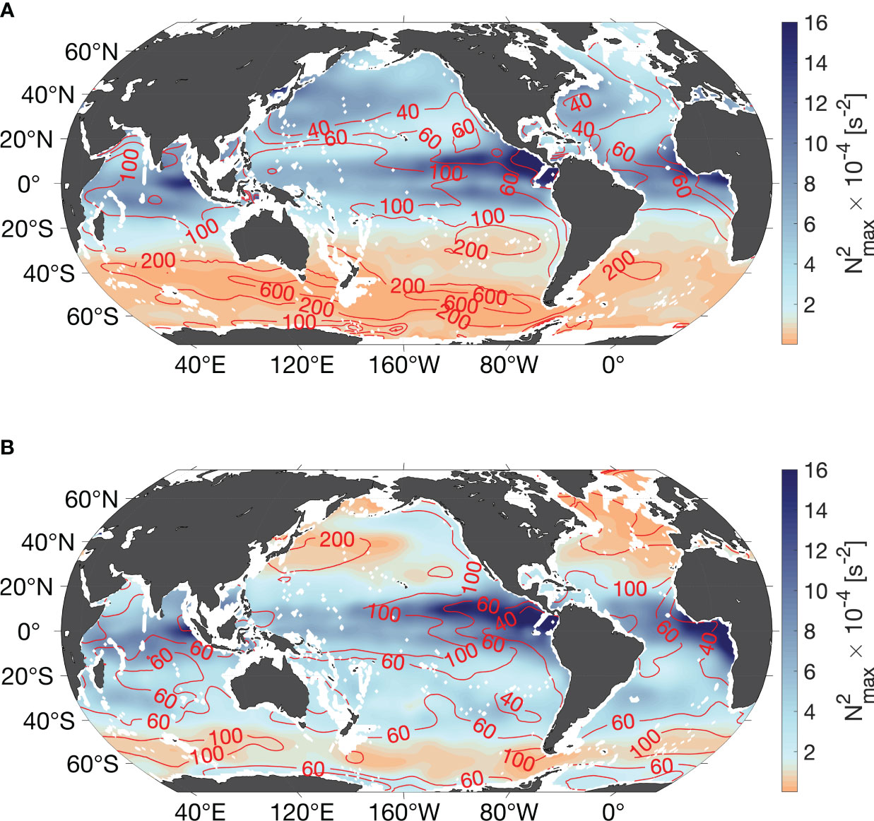
Figure 2 Mean vertical stratification maximum and its depth. (A) Mean vertical stratification maximum in July-September and (B) in January-March. Red contour lines mark the corresponding mean depth in meters.

High stratification values are accompanied by shallow depths of the vertical stratification maxima in most areas. The depths in the tropical oceans range from around 40-100 m, shoaling from west to east. The Northern Hemisphere reveals a distinct seasonal cycle of the depth of the stratification maximum with around 40 m in JAS (Figure 2A) and deeper than 200 m in JFM (Figure 2B). A similar cycle is found in the Southern Ocean, where its depths span from 60-100 m in JFM, reaching beyond 600 m in JAS (Figure 2).

3.2 Observed changes in vertical stratification maximum strength and depth

The above mean state residuals of monthly data (Figure 2) are used to derive multi-year trends of depth and stratification strength (Figure 3).

Figure 3 Trend of vertical stratification maximum. (A) Trend of vertical stratification maximum in July-September and (B) trend of the corresponding zonal mean. (C, D) same as in (A, B) but for January-March. Contour lines in (A, C) show the respective mean vertical stratification maximum given in ×10^-4 s^-2. Labels of the contours have to be multiplied by 10^-4. Dotted areas refer to where the trend is not of 95% significance. Shading in (B, D) depicts the 95% confidence interval.

The North Pacific Ocean is undergoing substantial changes by vast increasing stratification in both seasons (1.5×10^-4 s^-2 decade^-1 equivalent to 40-50% decade^-1 in JAS) especially around 10°N stratification increases by 2.5×10^-4 s^-2 decade^-1 (equivalent to ~10% decade^-1, Figure 3). On the contrary, the increase of the South Pacific Ocean stratification maximum is small in JAS and in many areas the trend is not statistically significant (see Methods). In JFM the South Pacific Ocean reveals a dipole pattern with a large rise of stratification in the southwest (3×10^-4 s^-2 decade^-1) and a decline in the central-eastern tropical South Pacific Ocean. Along the eastern continental slope, the eastern boundary upwelling system experiences enhanced stratification. The stratification maximum in the eastern equatorial Pacific decreases intensely in JFM (-2×10^-4 s^-2 decade^-1, Figure 3).

Changes in the Atlantic Ocean are substantially different compared to those in the Pacific Ocean. The subtropical North Atlantic Ocean is marked by reduced stratification in JAS (-0.6×10^-4 s^-2 decade^-1, Figure 3A) and slightly less in JFM (Figure 3C). Only the Senegalo-Mauritanian upwelling region shows strengthening stratification in JFM. Poleward of 40°N, the northeastern North Atlantic stratification is slightly increasing during JAS. In JFM this positive trend is weaker but reaches further south. The eastern tropical Atlantic stratification intensifies (>2×10^-4 s^-2 decade^-1) in JAS and shows a less clear picture in JFM. The South Atlantic is dominated by a north-south dipole in JAS with strengthening stratification equatorward of 20°S and a weakly, significantly decreasing trend further south (Figure 3A). In JFM, we find declining stratification around 30°S-40°S and no continuous large-scale changes otherwise (Figure 3C).

The Indian Ocean has no large-scale areas of significant trends. Nonetheless, the JAS stratification north of 20°S reveals a positive trend. In JFM, the tropical Indian Ocean depicts a decreasing stratification maximum. South of the tropics, a small east-west dipole shows reduced stratification in the west and opposite in the east (Figure 3C).

To address a more global aspects of upper-ocean stratification changes, zonal mean fields of the observed trends are estimated. The trend of the global zonal mean of vertical stratification maxima is mostly positive in the Northern Hemisphere for both seasons (Figures 3B, D). The North Pacific dominates over the reversed trend in the Atlantic Ocean. Around 30°N the decreasing stratification of the North Atlantic Ocean becomes apparent in the trend of the zonal mean, in particular in JAS due to the larger magnitude of decrease in Atlantic Ocean stratification. The Southern Hemisphere encompasses almost no trends in the zonal mean in JAS (Figure 3B), while the summer JFM trend of the zonal mean shows a statistically significant strengthening stratification (Figure 3D).

There are many smaller scale regions that defy these general patterns. Owing the mapping scales, the oceanic structure might even be more heterogenous, despite the large-scale variation taking place. Summarizing the detailed description above, the observed overarching patterns are the Northern Hemisphere stratification intensification in summer and winter while the Southern Hemisphere becomes more stratified in summer only.

Next to stratification strength, the depth of the vertical stratification maximum is of importance. For both seasons, its depth trend indicates a large-scale shoaling in many regions of the global oceans (5-20 m decade^-1, Figure 4). Some areas as the tropical Pacific or the subtropical North Atlantic depict a deepening instead. Yet, in most areas the trends are not significant. Largest changes are observed in the Southern Ocean along the Antarctic Circumpolar Current in JAS and in the subpolar North Atlantic Ocean in JFM (Figures 4A, C). The trend of the zonal mean of the depth of the vertical stratification maximum in JAS shifts sign around 55°S. This can be linked to meridional shifts of the frontal zone which is found to be migrating southward and is associated to enhanced and poleward displaced westerly winds (Fyfe and Saenko, 2006; Chapman et al., 2020). Weak but statistically significant shoaling is present in the North Pacific Ocean during both seasons. The zonal mean trends of the stratification maximum depth demonstrate a surprising strong symmetry between the hemispheric respective seasons: Weak summer stratification maximum depth changes and pronounced shoaling during winter (Figures 4B, D).

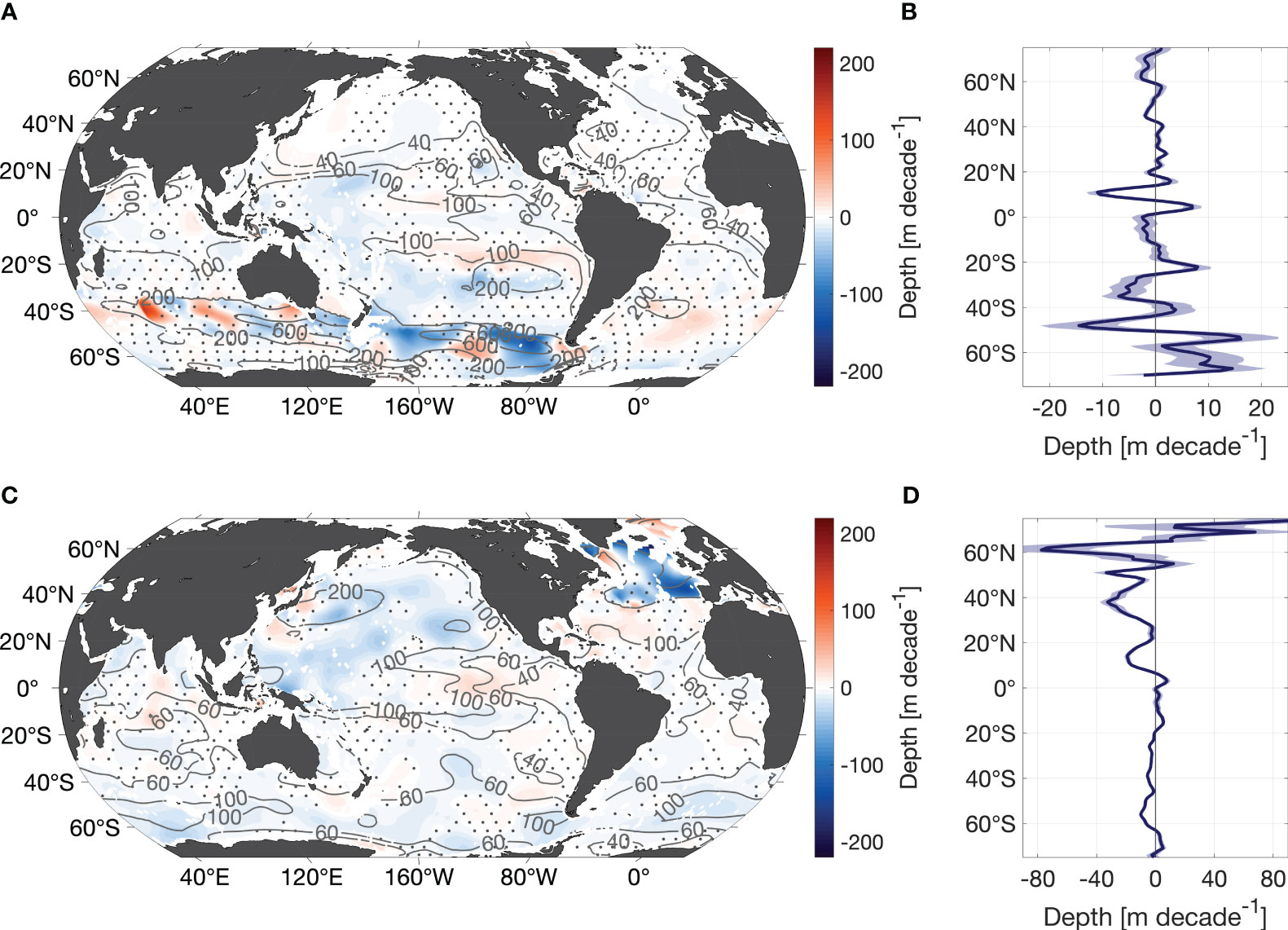
Figure 4 Trend of depth of the vertical stratification maximum. (A) Trend of the depth of the vertical stratification maximum in July-September and (B) trend of the corresponding zonal mean. (C, D) same as in (A, B) but for January-March. Contour lines in (A, C) show the respective mean fields in m. Dotted areas refer to where the trend is not of 95% significance. Shading in (B, D) depicts the 95% confidence interval.

3.3 Mixed layer variations

To better understand the origin of the observed changes of the vertical stratification maximum, we investigate changes of the mixed layer representing the interface between the stratified ocean and atmosphere. The parameters analyzed here include the mixed layer temperature (MLT), mixed layer salinity (MLS, Figure 5) and mixed layer depth (MLD, Figure 6). Mixed layer density changes can be inferred from the respective salinity and temperature trends. MLT and MLS trend patterns are similar in both seasons. The mixed layer is experiencing a vast and intense warming on the order of 1°C decade^-1 (Figures 5A, C). This warming is exceeded in the northeastern North Pacific in JAS and southwestern South Pacific in JFM (2°C decade^-1). The mixed layer is cooling in few regions in the Southern Ocean and the subpolar North Atlantic during both seasons. The subpolar North Atlantic has recently been exposed to a cooling period which is suggested to arise from a slowdown of the Atlantic Meridional Overturning Circulation and to be associated to the North Atlantic Oscillation (Robson et al., 2016; Caesar et al., 2018; Bulgin et al., 2020). This mixed layer cooling occurs where the stratification is decreasing in the subpolar North Atlantic and its impact is weakened by the exhibited mixed layer freshening. The freshening trend is most likely associated with the freshwater flux of glacial melt and melting sea ice (de Steur et al., 2018; Rühs et al., 2021). Further isolated intense cooling is observed in the eastern tropical Pacific cold tongue area in JAS (-2.5°C decade^-1). A cooling of the Pacific cold tongue is observed since the 1980s [e.g., Jiang and Zhu (2020); Latif et al. (2023)]. It is suggested to result from strengthened atmospheric deep convection over the warm pool regions in the western Pacific and south of North America, leading to anomalous vertical circular circulation and thereby causing a westward shift of the Walker circulation (Jiang and Zhu, 2020). This produces a strong divergence over the eastern Pacific, shoaling the thermocline and thus, enhanced cooling of the Pacific cold tongue. Recently, Latif et al. (2023) found that intensifying trade winds impact ocean dynamical processes and air-sea heat exchange, and thereby, counterbalance the externally forced sea surface temperature warming. Another potential reason for the cold tongue cooling might be related to the Pacific Decadal Oscillation. It was mostly in a negative phase during our observation period which manifests in a large-scale cooling in the tropical Pacific (Latif et al., 2023).

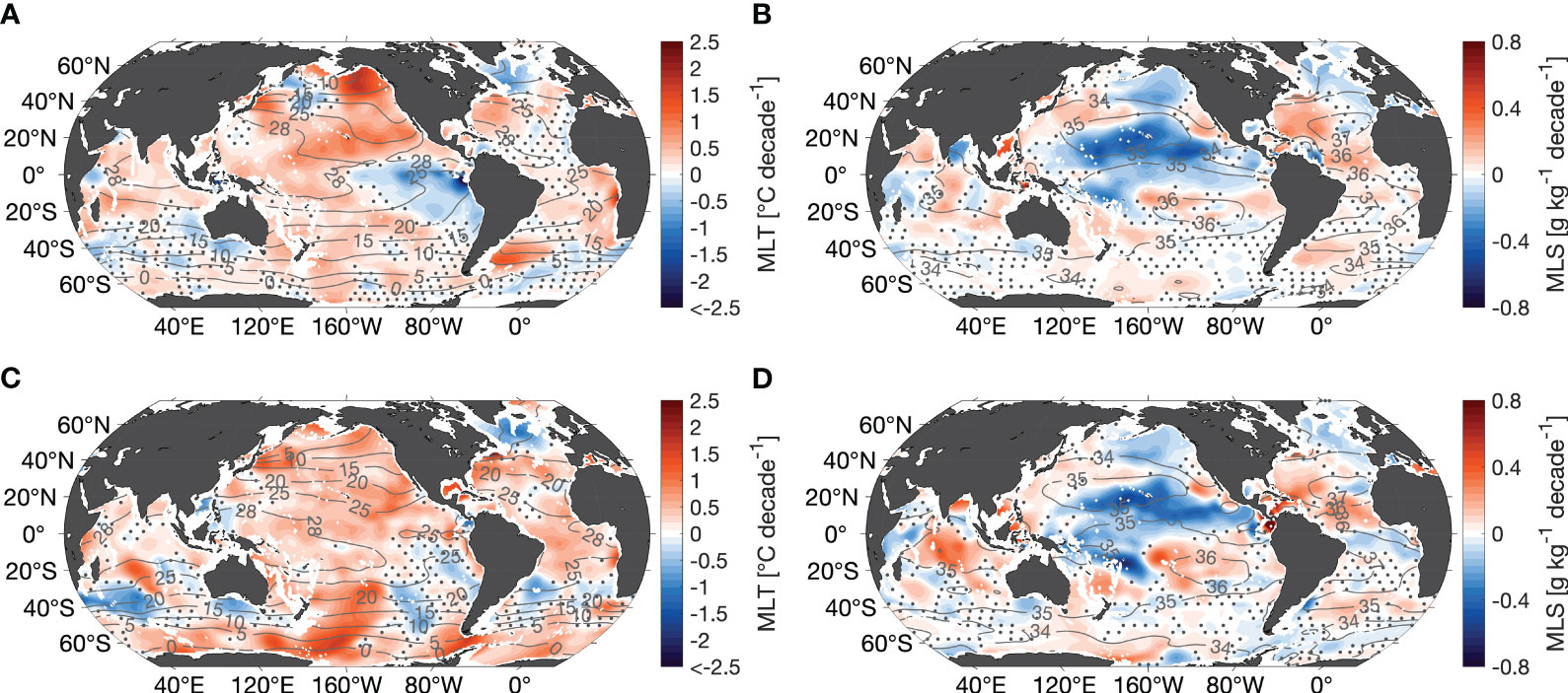
Figure 5 Trends of temperature and salinity of the mixed layer. (A) Trend of mixed layer temperature and (B) mixed layer salinity in July-September. (C, D) same as in (A, B) but for January-March. Labelled contour lines show the corresponding mean field in °C and g kg^-1 correspondingly. Dotted areas refer to where the trend is not of 95% significance.

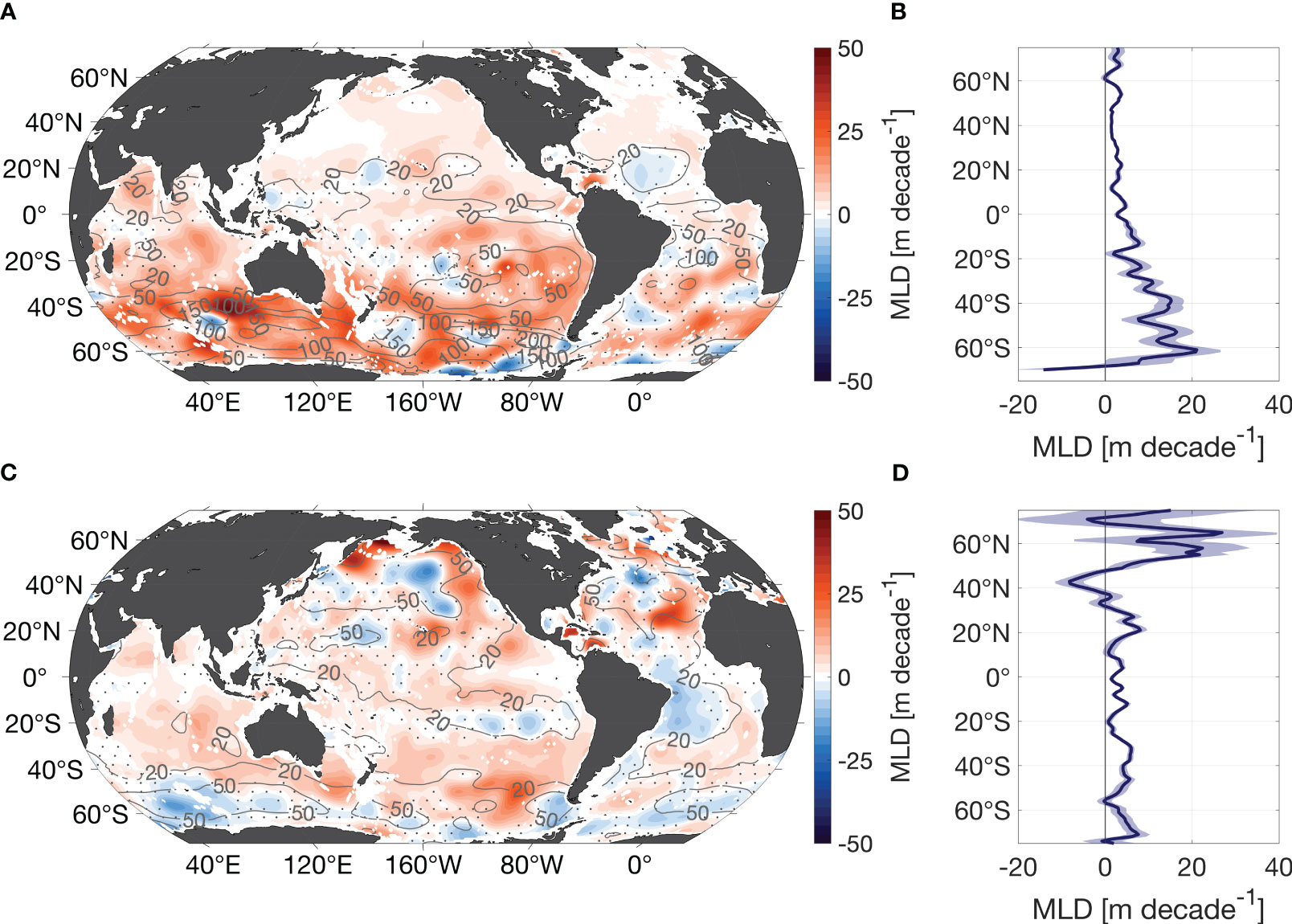
Figure 6 Trend of mixed layer depth. (A) Trend of the mixed layer depth in July-September and (B) trend of the corresponding zonal mean. (C, D) same as in (A, B) but for January-March. Contour lines in (A, C) show the respective mean fields. Dotted areas refer to where the trend is not of 95% significance. Shading in (B, D) depicts the 95% confidence interval.

The mixed layer is freshening in the subtropical North and tropical West Pacific Ocean in both seasons (0.5 g kg^-1 decade^-1, Figures 5B, D). A potential cause for the salinity decrease is enhanced freshwater flux in the central Pacific Ocean (Ke-xin and Fei, 2022). In the South Pacific Ocean, the salinity maximum water is becoming more saline which is consistent with the findings of Bingham et al. (2019). For the period of 2011-2019 they found advection changes of the subtropical gyre, South Equatorial Undercurrent, Ekman transport and Ekman pumping leading to a more saline salinity maximum water.

A synopsis of the MLT, MLS and vertical stratification maximum changes indicate enhancing stratification when the mixed layer is warming and freshening at the same time and thus, leading to a density reduction (e.g., subtropical North Pacific Ocean in both seasons, Figures 3, 5). When MLT and MLS show counterbalancing changes, it depends on which component has the largest effect on density and in turn, lead to the observed stratification adjustment (Supplementary Figure S7). In the subtropical North Atlantic Ocean, northwest of the salinity maximum, MLS increases (0.3 g kg^-1 decade^-1; Figures 5B, D), coexistent with the reduction of stratification in JAS and JFM (Figure 3). The location of the more saline mixed layer could be a result of the poleward shift of the North Atlantic salinity maximum formation region recently suggested for the period of 1979-2012 (Yu et al., 2018; Liu et al., 2019).

The counterbalancing effect of salinity in the North Atlantic becomes more evident from thermal and haline contributions to the trend of vertical stratification maximum (Supplementary Figure S7). In both seasons the trend of the haline contribution is negative while the trend of the thermal contribution is weakly negative in JAS and weakly positive in JFM in the North Atlantic (Supplementary Figure S7).

Also, the MLS of the tropical Indian Ocean increases, especially in JFM. Yet, it is the MLT changes that mainly mirror the stratification changes in the Indian Ocean. MLT trend patterns are comparable to the trend pattern of the Indian Ocean heat content anomaly for the upper 700 m presented by Roxy et al. (2020). Decadal variations of upper-ocean heat content in the Indian Ocean are linked to a La Niña-like climate shift and intensified heat transport via the Indonesian Throughflow (Liu et al., 2016).

The Southern Ocean depicts weak and barely significant MLS trends. Therefore, Southern Ocean MLT changes seems to be the main contributor to the observed stratification change (cf. Supplementary Figure S7). Nonetheless, since stratification changes in JAS are weak although MLT is rising, an impact by salinification cannot be ruled out.

The last mixed layer parameter examined, the MLD, is deepening globally in a surprising uniform pattern with few variations and a distinct seasonal pattern (Figure 6). Summer mixed layers are slightly deepening (5-10 m decade^-1) while winter mixed layers show a more pronounced deepening (30-50 m decade^-1) in both hemispheres. The trends of the zonal means also portray this symmetric behavior (Figures 6B, D).

3.4 Strain and isopycnal heave

Stratification changes of its vertical maximum may not only arise from changing mixed layer characteristics, but also from isopycnal heave and associated strain changes [vertical displacement of isopycnals (Bindoff and McDougall, 1994; Huang, 2015; Roch et al., 2021)] within the stratified ocean. Due to isopycnal movement, vertical density gradients change by squeezing/stretching of the isopycnal layers. This leads to enhanced/reduced stratification and affects the vertical stratification maximum. Basin-wide zonal mean trends show different isopycnal behavior among the three oceans and are compared to corresponding zonal mean trends of MLD and stratification maximum depth (Figures 7–9).

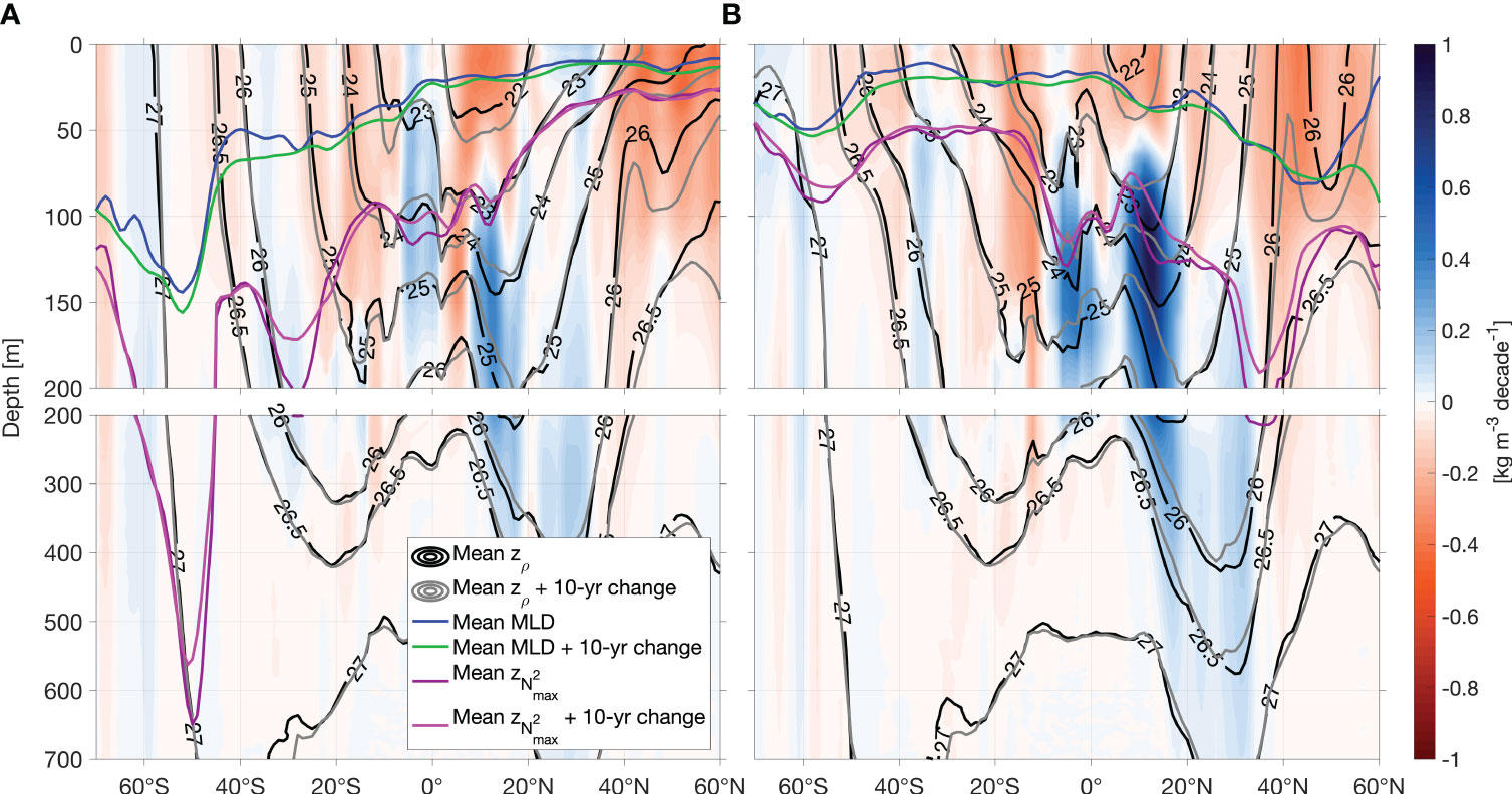
Figure 7 Changes of isopycnal heave in Pacific Ocean. (A) Trend of density in the Pacific in July-September and (B) in January-March for the time period of 2006-2021. Note, reddish colors imply a density reduction (i.e., warming and/or freshening) and blue colors a density enhancement. Additionally, zonal mean depths of isopycnals are shown in black, and mean depths plus 10-year changes in grey. The 10-year changes are derived from the trend. Blue lines show the zonal mean mixed layer depth (MLD), green lines refer to the mean MLD plus 10-year changes. Purple lines denote the zonal mean pycnocline depth ($z_{N_{max}^2}$) and pink lines the corresponding mean depth plus 10-year changes.

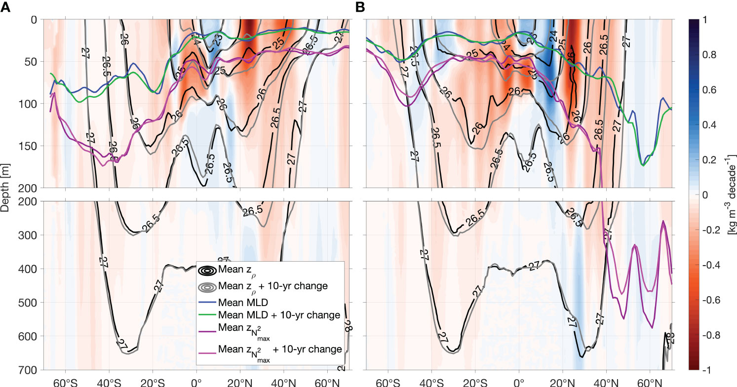
Figure 8 Changes of isopycnal heave in Atlantic Ocean. (A) Trend of density in the Atlantic in July-September and (B) in January-March for the time period of 2006-2021. Note, reddish colors imply a density reduction (i.e., warming and/or freshening) and blue colors a density enhancement. Additionally, zonal mean depths of isopycnals are shown in black, and mean depths plus 10-year changes in grey. The 10-year changes are derived from the trend. Blue lines show the zonal mean mixed layer depth (MLD), green lines refer to the mean MLD plus 10-year changes. Purple lines denote the zonal mean pycnocline depth ($z_{N_{max}^2}$) and pink lines the corresponding mean depth plus 10-year changes.

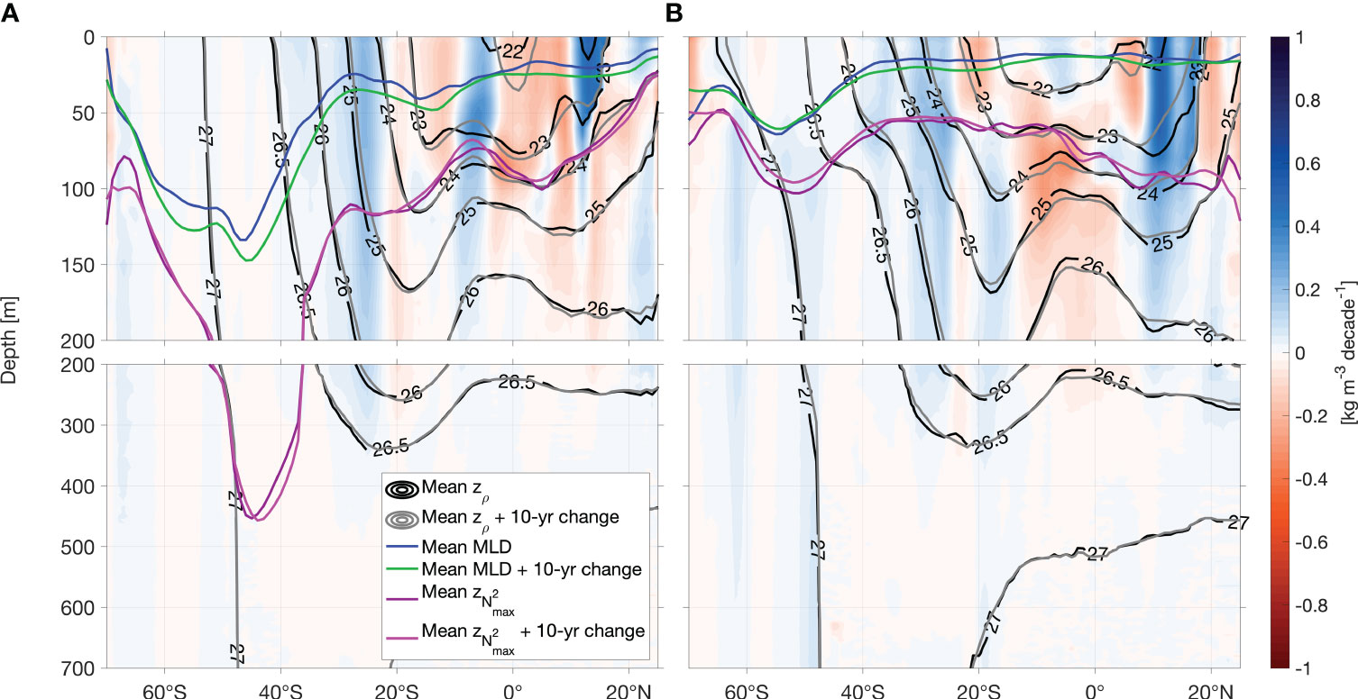
Figure 9 Changes of isopycnal heave in Indian Ocean. (A) Trend of density in the Indian Ocean in July-September and (B) in January-March for the time period of 2006-2021. Note, reddish colors imply a density reduction (i.e., warming and/or freshening) and blue colors a density enhancement. Additionally, zonal mean depths of isopycnals are shown in black, and mean depths plus 10-year changes in grey. The 10-year changes are derived from the trend. Blue lines show the zonal mean mixed layer depth (MLD), green lines refer to the mean MLD plus 10-year changes. Purple lines denote the zonal mean pycnocline depth ($z_{N_{max}^2}$) and pink lines the corresponding mean depth plus 10-year changes.

In many areas of the Pacific and Atlantic Oceans, we observe a mixed layer density reduction corresponding to a poleward migration and a downward movement of the isopycnals below the MLD (Figures 7, 8). Around the depth of the stratification maximum within the equatorial-subtropical North Pacific Ocean, the density trend is changing its sign (shoaling isopycnals: 20 m decade^-1, Figure 7). These opposing density trends in the upper and lower layers, lead to squeezing of isopycnal layers and corresponding volume changes. This is observed in both seasons in the subtropical North Pacific Ocean and contributing to the observed stratification increases (Figure 3). In the subtropical South Pacific isopycnal heave is weak in both seasons. Opposing behavior of the Pacific Ocean MLD and stratification maximum depth in JAS and JFM lead to a squeezing of the layer in between (Figure 7).

In the Atlantic Ocean, the uneven isopycnal deepening induces a stretching of the isopycnal layers at the depth of the vertical stratification maximum (particularly within 20°N-30°N, Figure 8). Maximum deepening is observed on the 26.5 kg m^-3- and 26.0 kg m^-3-isopycnals in the centers of the North and South Atlantic subtropical gyres, respectively, in both seasons. Since we observe the largest deepening at depth in the subtropics, this implies that next to the surface density reduction, another process has to be involved. Wind stress curl changes can induce pure heaving (Bindoff and McDougall, 1994; Huang, 2015). Indeed, the deepening of isopycnals in the subtropical gyres indicate downwelling favorable conditions which fits to identified long-term intensification of the North Atlantic’s subtropical high (Li et al., 2012). Besides, observations indicate that volume anomalies of water masses within the North Atlantic Subtropical gyre as a result of transport divergence are associated with both: variations of thermocline depth and Ekman pumping (Evans et al., 2017). This points to wind-induced heave being a driver of the transport anomalies (Evans et al., 2017).

North of the equator (0°-20°N), increasing density leads to an isopycnal shoaling which further contributes to stretching of the layers surrounding the stratification maximum and therefore decreasing the stratification at this depth.

In the Atlantic Ocean, mixed layer and summer stratification maximum changes of the zonal mean mirror the changes described above (Figures 4, 6, 8). Below, the winter stratification maximum in the South Atlantic is deepening whereas the winter stratification maximum in the Northern Hemisphere is shoaling (almost 100 m decade^-1, Figure 7).

Density changes in the Indian Ocean vary from the patterns found in the other oceans. Poleward of 20°S in the Indian Ocean, a large-scale density increase is accompanied by an equatorward migration of isopycnal outcrops and a weak upwelling of isopycnals within the subtropics (Figure 9) during both seasons. The equatorial Indian Ocean is dominated by density reduction. Thus, the isopycnals are moving downward. North of 10°N, density is increasing again and the isopycnals are shoaling over time. These findings go along with a pronounced mixed layer deepening (10-20 m decade^-1), particularly in JAS.

3.5 Mean global changes of the vertical stratification maximum and the MLD

To provide global estimates of stratification changes of the upper-ocean, a 2-year median and IQR of all available profiles’ vertical stratification maxima, their depths and MLD anomalies during JAS and JFM are derived (Figure 10). For the Argo period, the global median of the vertical stratification maximum shows an intensification of 7-8% while the median of the MLD indicates a deepening of 4 m. Also, the lower and upper ends of the IQR of these two variables show a stratification increase and mixed layer deepening (Figure 10). The upper limits of the IQR of the data are changing even stronger than the median indicating a strong shift in the distribution. The depth of the vertical stratification maximum however, does not show a significant change when taking a global 2-year median.

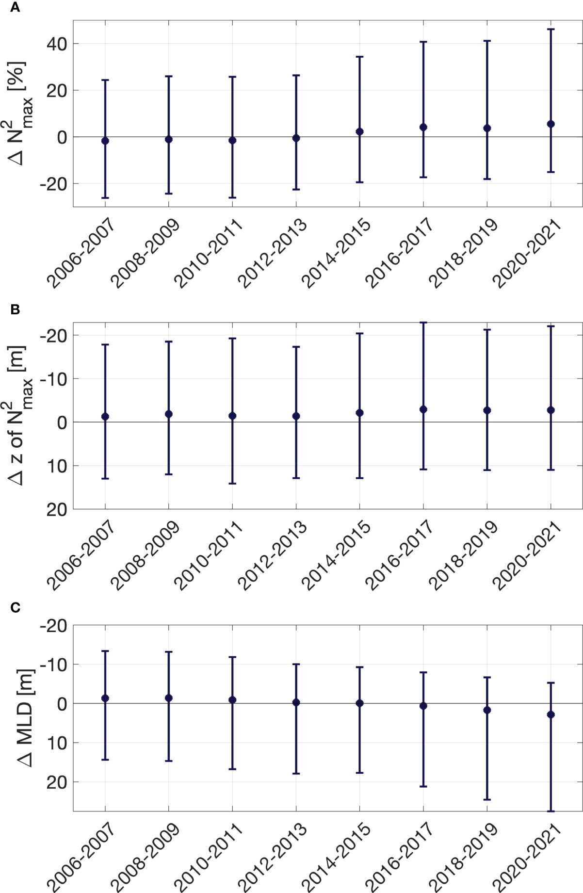
Figure 10 Global 2-year median of the vertical stratification maximum, its depth and MLD. Global 2-year median anomalies of the (A) vertical stratification maximum (B) its depth and (C) of the mixed layer depth (MLD). Anomalies are computed relative to the seasonal nearest grid point’s mean. Bars show the corresponding upper and lower limits of the interquartile range.

The increase of the stratification maximum of 7-8% is comparable to the strengthening of 6.1% of the upper 200 m of the water column by Yamaguchi and Suga (2019). Yet, their estimate is for the time period of 1960-2017 while our is for the years of 2006-2021 only. Currently, we are in the state of an intensified ocean surface warming (Garcia-Soto et al., 2021) and also the analysis of Yamaguchi and Suga (2019) showed an immense stratification increase for the period of 2010-2017. Therefore, it is possible that we observe such a large stratification increase in a rather short time period.

4 Discussion

4.1 Contributions of MLT, MLS and isopycnal heave to stratification changes

Our trend analysis of Argo data for the period 2006-2021 shows that on average the vertical stratification maximum in the Northern Hemisphere is strengthening in summer and winter whereas the Southern Hemisphere stratification maximum intensifies in summer (JFM) only (Figure 3). This is accompanied by mixed layer deepening and warming throughout both seasons. Due to thicker mixed layers, the volume between the MLD and stratification maxima is contracting during both, winter and summer. The large-scale warming of the mixed layer of 1°C decade^-1 is consistent with satellite sea surface temperature data from 1981-2018 (Bulgin et al., 2020). Mixed layer warming rates among four consecutive periods from the 37-year time series demonstrate the largest warming trend during the period of 2010-2018 (with regionally trends up to 4°C decade^-1) (Bulgin et al., 2020).

In general, the findings reveal stratification increases can be linked to surface density reduction mainly due to mixed layer warming and partly freshening as well as to squeezing of isopycnal layers (i.e., pure heave) at the depth of the vertical stratification maximum (e.g., subtropical North Pacific). Nevertheless, the global maps highlight several regional differences of stratification changes during the analyzed period indicating that decadal to multidecadal climate variability is most likely responsible for some of the observed variations. The results show warming of the ocean surface does not necessarily imply intensifying stratification maxima on decadal time scales as it was demonstrated for longer time periods (1990-2015 by Somavilla et al., 2017). In some regions the mixed layer warming-induced density reduction is counterbalanced by a salinity increase which then in turn occurs along with a reduction of stratification if the salinity increase is large enough (e.g., subtropical North Atlantic, Figures 3, 5, Supplementary Figure S7). It should be noted that our findings of the MLS changes do not suggest an amplification of the hydrological cycle as determined by Durack and Wijffels (2010). However, this can be attributed to the different investigated time periods and observation lengths. It is most likely that we here observe a multi-year climate variability as we focus on the past 16 years. Mixed layer changes may be associated with variations in advection and freshwater fluxes (Sprintall and Cronin, 2009). Apart from MLT and MLS variations, stratification is impacted by isopycnal heave. Stretching and squeezing of isopycnal layers is caused by wind stress curl changes (Bindoff and McDougall, 1994; Huang, 2015) and the related volume changes affect the stratification (e.g., contraction of volume in the North Pacific leading to enhanced stratification and stretching of isopycnals in the North Atlantic causing a reduction of stratification, Figures 3, 7, 8).

4.2 Mixed layer deepening and stratification increase

Changes of stratification have been addressed by analyzing MLT, MLS and isopycnal heave. The large-scale vast mixed layer deepening will be addressed in the following. Mixed layer deepening might modulate upper-ocean stratification. As indicated in the introduction, model studies have suggested that on-going warming and ocean stratification intensification may lead to thinner mixed layers (Capotondi et al., 2012). Recent observations indicate long-term intensifying stratification (Yamaguchi and Suga, 2019; Li et al., 2020; Sallée et al., 2021) does not have to go along with thinner mixed layers (Somavilla et al., 2017; Sallée et al., 2021). In fact, the summer mixed layer is deepening for the period 1970-2018 (Sallée et al., 2021). For the much shorter Argo observation period, we identify a significant mixed layer deepening in most regions as well as on global scale. Whether this is part of the on-going long-term deepening trend or a period of climate variability remains to be investigated with the prolonging observations of the Argo array.

We observe a symmetric seasonal mixed layer deepening in both hemispheres. This large-scale deepening is more pronounced in winter than in summer and only small limited regions defy the global trend. Warmer and thicker mixed layers contribute to a stronger vertical stratification maximum. This can be explained as follows: oceanic warming from atmospheric forcing creates a vertical temperature gradient and thus density gradient, leading to a pronounced increase of depth average stratification and a slight increase of the stratification maximum. A subsequent wind-induced deepening of the upper well-mixed layer reduces the distance between the bottom of mixed layer and vertical stratification maximum. This contraction results in an upward shift and strengthening of the vertical stratification maximum. In summer, the stratification maximum demonstrates only weak changes whereas the winter stratification maximum shows a pronounced shoaling trend. This generates a squeezing of the layer between the deepening mixed layer and the vertical stratification maximum, being more intense during winter.

As the mixed layer deepens, the mixed layer heat content increases stronger than expected from sea surface warming of satellite measurements alone. Larger ocean heat content could contribute to enhanced hurricane activity (Trenberth et al., 2018). Since the winter mixed layer thickens stronger than the summer mixed layer, the seasonal cycle of the MLD is amplified, which impacts the subduction of mode waters. The largest winter MLD increases are situated poleward of 40°. Mode waters are mainly formed by the lateral induction part of the subduction equation (Marshall et al., 1993; Hanawa and Talley, 2001; Karstensen and Quadfasel, 2002). If the seasonal cycle and the meridional gradient of the MLD are enhancing, lateral induction is intensifying and subtropical mode water volume increases due to isopycnal heaving (Häkkinen et al., 2015; Häkkinen et al., 2016). These processes may help to explain why mode waters are identified as warming hot spots during the Argo period (Kolodziejczyk et al., 2019).

Possibilities of increased MLD are changing buoyancy fluxes, but since the mixed layer is warming the buoyancy fluxes would yield the wrong sign. Therefore, we conclude wind is likely the main contributor. There are two mechanisms by which wind might contribute to enhanced MLD: increased turbulent mixing due to stronger winds and increased Ekman convergence due to intensified cyclonic wind stress curl. It is well-known that global trend analysis of wind is uncertain with a tendency to increased wind speeds over the ocean (Torralba et al., 2017). We investigated changes of the wind speed and its variability of different products (Supplementary Figures S5, S6). Despite the high uncertainty of wind products, the results indicate wind changes from current wind datasets cannot explain the nearly unanimous global mixed layer deepening. Some regions as in the Northern Hemisphere in JFM indicate enhanced wind speed and variability which might contribute to thicker winter mixed layers. Yet, there are also many areas, where the wind variability seems to decrease. Intensifying subtropical highs are suggested in a warming climate (Li et al., 2012). Besides, observations (2005-2014) indicate an intensifying South Pacific Gyre Circulation caused by anomalous Ekman convergence (Roemmich et al., 2016). Such changes are associated with wind stress curl changes driving Ekman convergences and therefore impacting MLD.

The question why the mixed layer is deepening cannot be solved within this study. Nevertheless, changes of the wind fields are a possible contributor. Different wind regimes rule in different places and in different seasons. Other parameters of wind can have an influence, such as frequency, maximum magnitudes, timings, mid-latitude winter storms, tropical cyclones, etc. To just name a few variables that highlight the difficulties we have to deal with.

The described and analyzed large-scale pattern indicate various forces at play in the upper-ocean stratification, with MLT increase playing into most observed changes. Nevertheless, regional differences are large and regionally as well as temporally varying forces can play an important role. The identified changes cannot solely be linked to one global trend. While the data used here is de-weighting ENSO, other climate variations, as Pacific Decadal Oscillation, Atlantic Meridional Oscillation, Southern Annular Mode, North Atlantic Oscillation play a role in determining the regional to basin scale trend patterns.

The Argo project allows us to investigate upper-ocean changes for the past 16 years. Uncertainties from this product have to be kept in mind. There might be gaps in the data in some regions for some periods. For example, the central subtropical South Pacific has some regions where the maximum time span within a 2° x 2° grid box covered by Argo profiles is 6 years or less (Supplementary Figure S1). Trends in areas like this should be treated with caution. Nevertheless, most areas show a sufficient amount and time span of available profiles per grid box (Supplementary Figure S1). Besides, the estimated trends have been compared to actual time series of JAS and JFM vertical stratification maximum and MLD anomalies (Supplementary Figures S8-S11). The regional time series confirm that the identified trend yields reasonable results. Indeed, many regions reveal continuous intensification of the vertical stratification maximum as well as ongoing mixed layer deepening. Hence, for the Argo observation period of 16 years we are able to show significant trends of upper-ocean stratification and mixed layer properties. To determine whether these changes and regional differences are part of the ongoing climate warming, the Argo time series has to be continuously updated.

5 Conclusion

For the Argo observation period, the vertical stratification maximum is intensifying on a global average by 7-8%. Even though there are large regional differences, the global signal suggests an increasing de-coupling of the surface ocean from the ocean interior in the past 16 years. The observed modified stratification can be associated with a warmer and thicker mixed layer. The salinity changes either contribute or counteract the warming-induced density reduction, depending on the region. Additionally, the isopycnal heave plays a role in adjusting the vertical stratification maximum and is likely to have been impacted by wind stress curl-driven changes. The deepening of the mixed layer and squeezing of the layers below down to the vertical stratification maxima in summer and winter, have the potential to impact mode water formation processes, ocean ventilation and mixing, and further biological consequences. Impacts on nutricline, subsurface oxygen levels and therefore the marine ecosystem are expected to be manifold and regionally diverse. The presented analysis can help identify model – observation discrepancies concerning MLD and stratification, determine its causes and help to improve model predictions and projections. Since many ecological and biogeochemical processes in the upper-ocean are impacted by MLD and stratification, their correct representation in climate models is necessary to better understand looming changes to ecosystem and biogeochemistry in the ocean.

Data availability statement

The analyzed datasets are publicly available. This data can be found here: Argo (2021). Argo float data and metadata from Global Data Assembly Centre (Argo GDAC) - Snapshot of Argo GDAC of December 10st 2021. SEANOE. doi: 10.17882/42182#90179. The Ocean Nino Index (ONI) by Trenberth et al. (2020): https://psl.noaa.gov/data/correlation/oni.data. All necessary codes for this study are available at: Roch, Marisa, Brandt, Peter, & Schmidtko, Sunke. (2023). Software used in "Recent large-scale mixed layer and vertical stratification maxima changes" (Version 3). Zenodo. https://doi.org/10.5281/zenodo.8382701. Datasets used in the Supplementary Materials: M158 CTD data from Brandt, Subramaniam, Schmidtko, Krahmann (2022): Physical oceanography (CTD) during METEOR cruise M158. PANGAEA, https://doi.org/10.1594/PANGAEA.952354. CCMP wind data from Remote Sensing Systems (Wentz et al., 2015): https://www.remss.com/measurements/ccmp/. ERA5 data by Hersbach et al. (2018): https://cds.climate.copernicus.eu/cdsapp#!/dataset/reanalysis-era5-single-levels?tab=overview and the global wind product of E. U. Copernicus Marine Service Information: https://data.marine.copernicus.eu/product/WIND_GLO_WIND_L4_REP_OBSERVATIONS_012_006/description.

Author contributions

MR: Methodology, Software, Writing – original draft, Writing – review & editing, Conceptualization, Formal Analysis, Investigation, Visualization. PB: Writing – review & editing, Investigation. SS: Methodology, Software, Writing – review & editing, Investigation.

Funding

The authors declare financial support was received for the research, authorship, and/or publication of this article. This study was supported by the EU H2020 TRIATLAS project under grant agreement 817578.

Acknowledgments

We acknowledge the use of the Argo observation dataset, the ONI by Trenberth and National Center for Atmospheric Research Staff (2020), the use of CCMP wind data from Remote Sensing Systems (Wentz et al., 2015), the use of ERA5 data by Hersbach et al. (2018) and the use of the global wind product of E. U. Copernicus Marine Service Information.

Conflict of interest

The authors declare that the research was conducted in the absence of any commercial or financial relationships that could be construed as a potential conflict of interest.

Publisher’s note

All claims expressed in this article are solely those of the authors and do not necessarily represent those of their affiliated organizations, or those of the publisher, the editors and the reviewers. Any product that may be evaluated in this article, or claim that may be made by its manufacturer, is not guaranteed or endorsed by the publisher.

Supplementary material

The Supplementary Material for this article can be found online at: https://www.frontiersin.org/articles/10.3389/fmars.2023.1277316/full#supplementary-material

References

Akima H. (1970). A new method of interpolation and smooth curve fitting based on local procedures. J. ACM (JACM) 17, 589–602. doi: 10.1145/321607.321609
Argo (2021). Argo float data and metadata from Global Data Assembly Centre (Argo GDAC) - Snapshot of Argo GDAC of December 10st 2021 (SEANOE). doi: 10.17882/42182#90179
Balaguru K., Foltz G. R., Leung L. R., Emanuel K. A. (2016). Global warming-induced upper-ocean freshening and the intensification of super typhoons. Nat. Commun. 7, 13670. doi: 10.1038/ncomms13670
Bindoff N. L., McDougall T. J. (1994). Diagnosing climate change and ocean ventilation using hydrographic data. J. Phys. Oceanogr. 24, 1137–1152. doi: 10.1175/1520-0485(1994)024<1137:dccaov>2.0.co;2
Bingham F. M., Busecke J. J. M., Gordon A. L. (2019). Variability of the South Pacific subtropical surface salinity maximum. J. Geophys. Res. Oceans 124, 6050–6066. doi: 10.1029/2018JC014598
Bopp L., Lévy M., Resplandy L., Sallée J. B. (2015). Pathways of anthropogenic carbon subduction in the global ocean. Geophys. Res. Lett. 42, 6416–6423. doi: 10.1002/2015GL065073
Bulgin C. E., Merchant C. J., Ferreira D. (2020). Tendencies, variability and persistence of sea surface temperature anomalies. Sci. Rep. 10, 7986. doi: 10.1038/s41598-020-64785-9
Caesar L., Rahmstorf S., Robinson A., Feulner G., Saba V. (2018). Observed fingerprint of a weakening Atlantic Ocean overturning circulation. Nature 556, 191–196. doi: 10.1038/s41586-018-0006-5
Capotondi A., Alexander M. A., Bond N. A., Curchitser E. N., Scott J. D. (2012). Enhanced upper ocean stratification with climate change in the CMIP3 models. J. Geophys. Res. Oceans 117, C04031. doi: 10.1029/2011JC007409
Chapman C. C., Lea M. A., Meyer A., Sallée J. B., Hindell M. (2020). Defining Southern Ocean fronts and their influence on biological and physical processes in a changing climate. Nat. Clim. Chang. 10, 209–219. doi: 10.1038/s41558-020-0705-4
Cronin M. F., Bond N. A., Thomas Farrar J., Ichikawa H., Jayne S. R., Kawai Y., et al. (2013). Formation and erosion of the seasonal thermocline in the Kuroshio Extension Recirculation Gyre. Deep Sea Res. 2 Top. Stud. Oceanogr. 85, 62–74. doi: 10.1016/j.dsr2.2012.07.018
Desbruyères D., McDonagh E. L., King B. A., Thierry V. (2017). Global and full-depth ocean temperature trends during the early twenty-first century from argo and repeat hydrography. J. Clim. 30, 1985–1997. doi: 10.1175/JCLI-D-16-0396.1
de Steur L., Peralta-Ferriz C., Pavlova O. (2018). Freshwater export in the east Greenland current freshens the North Atlantic. Geophys. Res. Lett. 45, 13,359–13,366. doi: 10.1029/2018GL080207
Durack P. J., Wijffels S. E. (2010). Fifty-year trends in global ocean salinities and their relationship to broad-scale warming. J. Clim. 23, 4342–4362. doi: 10.1175/2010JCLI3377.1
Evans D. G., Toole J., Forget G., Zika J. D., Garabato A. C. N., George Nurser A. J., et al. (2017). Recent wind-driven variability in atlantic water mass distribution and meridional overturning circulation. J. Phys. Oceanogr. 47, 633–647. doi: 10.1175/JPO-D-16-0089.1
Ferrari R., Boccaletti G. (2004). Eddy-mixed layer interactions in the ocean. Oceanography 17, 12–21. doi: 10.5670/oceanog.2004.26
Feucher C., Maze G., Mercier H. (2019). Subtropical mode water and permanent pycnocline properties in the world ocean. J. Geophys. Res. Oceans 124, 1139–1154. doi: 10.1029/2018JC014526
Fiedler P. C., Mendelssohn R., Palacios D. M., Bograd S. J. (2013). Pycnocline variations in the eastern tropical and north pacific 1958-2008. J. Clim. 26, 583–599. doi: 10.1175/JCLI-D-11-00728.1
Fiedler P. C., Talley L. D. (2006). Hydrography of the eastern tropical Pacific: A review. Prog. Oceanogr. 69, 143–180. doi: 10.1016/j.pocean.2006.03.008
Fyfe J. C., Saenko O. A. (2006). Simulated changes in the extratropical Southern Hemisphere winds and currents. Geophys. Res. Lett. 33, L06701. doi: 10.1029/2005GL025332
Garcia-Soto C., Cheng L., Caesar L., Schmidtko S., Jewett E. B., Cheripka A., et al. (2021). An overview of ocean climate change indicators: sea surface temperature, ocean heat content, ocean pH, dissolved oxygen concentration, arctic sea ice extent, thickness and volume, sea level and strength of the amoc (atlantic meridional overturning circulation). Front. Mar. Sci. 8, 642372. doi: 10.3389/fmars.2021.642372
Gill A. E. (1982). ““Use of Potential Temperature as a State Variable,”,” in Atmosphere-Ocean Dynamics (New York: Academic Press), 53–54.
Häkkinen S., Rhines P. B., Worthen D. L. (2015). Heat content variability in the North Atlantic Ocean in ocean reanalyses. Geophys. Res. Lett. 42, 2901–2909. doi: 10.1002/2015GL063299
Häkkinen S., Rhines P. B., Worthen D. L. (2016). Warming of the global ocean: Spatial structure and water-mass trends. J. Clim. 29, 4949–4963. doi: 10.1175/JCLI-D-15-0607.1
Hanawa K., Talley L. D. (2001). Chapter 5.4 mode waters. Int. Geophys. 77, 373–386. doi: 10.1016/S0074-6142(01)80129-7
Hersbach H., Bell B., Berrisford P., Biavati G., Horányi A., Muñoz Sabater J., et al. (2018). ERA5 hourly data on single levels from 1959 to present. Copernicus Climate Change Service (C3S) Climate Data Store (CDS). doi: 10.24381/cds.adbb2d47
Holte J., Talley L. (2009). A new algorithm for finding mixed layer depths with applications to argo data and subantarctic mode water formation. J. Atmos. Ocean Technol. 26, 1920–1939. doi: 10.1175/2009JTECHO543.1
Huang R. X. (2010). “Subduction and obduction,” in Ocean circulation: wind-driven and thermohaline processes (Cambridge, United Kingdom: Cambridge University Press), 512–536.
Huang R. X. (2015). Heaving modes in the world oceans. Clim. Dyn. 45, 3563–3591. doi: 10.1007/s00382-015-2557-6
IOC, SCOR, IAPSO. (2010). The International Thermodynamic equation of seawater - 2010: Calculation and use of thermodynamic properties, Manuals and Guides. 56, 196 pp. UNESCO. Available at http://www.TEOS-10.org.
Iselin C. O. (1939). The influence of vertical and lateral turbulence on the characteristics of the waters at mid-depths. Eos Trans. Am. Geophys. Union 20, 414–417.
Jiang N., Zhu C. (2020). Tropical Pacific cold tongue mode triggered by enhanced warm pool convection due to global warming. Environ. Res. Lett. 15, 054015. doi: 10.1088/1748-9326/ab7d5e
Johnston T. M. S., Rudnick D. L. (2009). Observations of the transition layer. J. Phys. Oceanogr. 39, 780–797. doi: 10.1175/2008JPO3824.1
Kaminski A. K., D’asaro E. A., Shcherbina A. Y., Harcourt R. R. (2021). High-resolution observations of the north pacific transition layer from a Lagrangian float. J. Phys. Oceanogr. 51, 3163–3181. doi: 10.1175/JPO-D-21-0032.1
Karstensen J., Quadfasel D. (2002). Formation of southern hemisphere thermocline waters : water mass conversion and subduction. J. Phys. Oceanogr. 32, 3020–3038. doi: 10.1175/1520-0485(2002)032<3020:FOSHTW>2.0.CO;2
Keeling R. F., Körtzinger A., Gruber N. (2010). Ocean deoxygenation in a warming world. Ann. Rev. Mar. Sci. 2, 199–229. doi: 10.1146/annurev.marine.010908.163855
Ke-xin L., Fei Z. (2022). Effects of a freshening trend on upper-ocean stratification over the central tropical Pacific and their representation by CMIP6 models. Deep Sea Res. 2 Top. Stud. Oceanogr. 195, 104999. doi: 10.1016/j.dsr2.2021.104999
Kolodziejczyk N., Llovel W., Portela E. (2019). Interannual variability of upper ocean water masses as inferred from argo array. J. Geophys. Res. Oceans 124, 6067–6085. doi: 10.1029/2018JC014866
Kwiatkowski L., Torres O., Bopp L., Aumont O., Chamberlain M., R. Christian J., et al. (2020). Twenty-first century ocean warming, acidification, deoxygenation, and upper-ocean nutrient and primary production decline from CMIP6 model projections. Biogeosciences 17, 3439–3470. doi: 10.5194/bg-17-3439-2020
Latif M., Bayr T., Kjellsson J., Lübbecke J. F., Nnamchi H. C., Park W., et al. (2023). Strengthening atmospheric circulation and trade winds slowed tropical Pacific surface warming. Commun. Earth Environ. 4, 249. doi: 10.1038/s43247-023-00912-4
Li G., Cheng L., Zhu J., Trenberth K. E., Mann M. E., Abraham J. P. (2020). Increasing ocean stratification over the past half-century. Nat. Clim. Chang. 10, 1116–1123. doi: 10.1038/s41558-020-00918-2
Li W., Li L., Ting M., Liu Y. (2012). Intensification of Northern Hemisphere subtropical highs in a warming climate. Nat. Geosci. 5, 830–834. doi: 10.1038/ngeo1590
Liu W., Xie S. P., Lu J. (2016). Tracking ocean heat uptake during the surface warming hiatus. Nat. Commun. 7, 10926. doi: 10.1038/ncomms10926
Liu H., Yu L., Lin X. (2019). Recent decadal change in the North Atlantic subtropical underwater associated with the poleward expansion of the surface salinity maximum. J. Geophys. Res. Oceans 124, 4433–4448. doi: 10.1029/2018JC014508
Llort J., Lévy M., Sallée J. B., Tagliabue A. (2019). Nonmonotonic response of primary production and export to changes in mixed-layer depth in the southern ocean. Geophys. Res. Lett. 46, 3368–3377. doi: 10.1029/2018GL081788
Lozier M. S., McCartney M. S., Owens W. B. (1994). Anomalous anomalies in averaged hydrographic data*. J. Phys. Oceanogr. 24, 2624–2638. doi: 10.1175/1520-0485(1994)024<2624:AAIAHD>2.0.CO;2
Marshall J. C., Nurser A. J. G., Williams R. G. (1993). Inferring the subduction rate and period over the North Atlantic. J. Phys. Oceanogr. 23, 1315–1329. doi: 10.1175/1520-0485(1993)023<1315:ITSRAP>2.0.CO;2
MathWorks Inc (2019) Help Center: Makima. Available at: https://de.mathworks.com/help/matlab/ref/makima.html (Accessed June 25, 2021).
McDougall T. J., Barker P. M. (2011). Getting started with TEOS-10 and the gibbs seawater (GSW) oceanographic toolbox. SCOR/IAPSO WG 127, 1–28.
McDougall T. J., Barker P. M. (2014). Comment on “Buoyancy frequency profiles and internal semidiurnal tide turning depths in the oceans” by B. King et al. J. Geophys. Res. Oceans 119, 9026–9032. doi: 10.1002/2014JC010066
Oschlies A., Brandt P., Stramma L., Schmidtko S. (2018). Drivers and mechanisms of ocean deoxygenation. Nat. Geosci. 11, 467–473. doi: 10.1038/s41561-018-0152-2
Rhein M., Rintoul S. R., Aoki S., Campos E., Chambers D., Feely R. A., et al. (2013). ““Observations: Ocean.,”,” in Climate Change 2013: The Physical Science Basis. Contribution of Working Group I to the Fifth Assessment Report of the Intergovernmental Panel on Climate Change. Eds. Stocker T. F., Qin D., Plattner G.-K., Tignor M., Allen S. K., Boschung J. (Cambridge: Cambridge University Press).
Robson J., Ortega P., Sutton R. (2016). A reversal of climatic trends in the North Atlantic since 2005. Nat. Geosci. 9, 513–517. doi: 10.1038/ngeo2727
Roch M., Brandt P., Schmidtko S., Vaz Velho F., Ostrowski M. (2021). Southeastern tropical atlantic changing from subtropical to tropical conditions. Front. Mar. Sci. 8, 748383. doi: 10.3389/fmars.2021.748383
Roemmich D., Church J., Gilson J., Monselesan D., Sutton P., Wijffels S. (2015). Unabated planetary warming and its ocean structure since 2006. Nat. Clim. Chang. 5, 240–245. doi: 10.1038/nclimate2513
Roemmich D., Gilson J., Sutton P., Zilberman N. (2016). Multidecadal change of the South Pacific Gyre circulation. J. Phys. Oceanogr. 46, 1871–1883. doi: 10.1175/JPO-D-15-0237.1
Roxy M. K., Gnanaseelan C., Parekh A., Chowdary J. S., Singh S., Modi A., et al. (2020). ““Indian Ocean Warming,”,” in Assessment of Climate Change over the Indian Region: A Report of the Ministry of Earth Sciences (MoES), Government of India. Eds. Krishnan R., Sanjay J., Gnanaseelan C., Mujumdar M., Kulkarni A., Chakraborty S. (Singapore: Springer Singapore), 191–206. doi: 10.1007/978-981-15-4327-2_10
Rühs S., Oliver E. C. J., Biastoch A., Böning C. W., Dowd M., Getzlaff K., et al. (2021). Changing spatial patterns of deep convection in the subpolar North Atlantic. J. Geophys. Res. Oceans 126, e2021JC017245. doi: 10.1029/2021JC017245
Sallée J. B., Pellichero V., Akhoudas C., Pauthenet E., Vignes L., Schmidtko S., et al. (2021). Summertime increases in upper-ocean stratification and mixed-layer depth. Nature 591, 592–598. doi: 10.1038/s41586-021-03303-x
Schmidtko S., Johnson G. C., Lyman J. M. (2013). MIMOC: A global monthly isopycnal upper-ocean climatology with mixed layers. J. Geophys. Res. Oceans 118, 1658–1672. doi: 10.1002/jgrc.20122
Schmidtko S., Stramma L., Visbeck M. (2017). Decline in global oceanic oxygen content during the past five decades. Nature 542, 335–339. doi: 10.1038/nature21399
Sérazin G., Tréguier A. M., de Boyer Montégut C. (2023). A seasonal climatology of the upper ocean pycnocline. Front. Mar. Sci. 10, 1120112. doi: 10.3389/fmars.2023.1120112
Somavilla R., González-Pola C., Fernández-Diaz J. (2017). The warmer the ocean surface, the shallower the mixed layer. How much of this is true? J. Geophys. Res. Oceans 122, 7698–7716. doi: 10.1002/2017JC013125
Sprintall J., Cronin M. F. (2009). “Upper Ocean Vertical Structure,” in Encyclopedia of Ocean Sciences. Eds. Steele. J. H., Thorpe S. A., Turekian K. K. (San Diego, California: Academic), 217–224. doi: 10.1016/B978-012374473-9.00627-5
Stommel H. (1979). Determination of water mass properties of water pumped down from the Ekman layer to the geostrophic flow below. Proc. Natl. Acad. Sci. 76, 3051–3055. doi: 10.1073/pnas.76.7.3051
Torralba V., Doblas-Reyes F. J., Gonzalez-Reviriego N. (2017). Uncertainty in recent near-surface wind speed trends: A global reanalysis intercomparison. Environ. Res. Lett. 12, 114019. doi: 10.1088/1748-9326/aa8a58
Trenberth K. E., Cheng L., Jacobs P., Zhang Y., Fasullo J. (2018). Hurricane Harvey links to ocean heat content and climate change adaptation. Earths Future 6, 730–744. doi: 10.1029/2018EF000825
Trenberth K. E., National Center for Atmospheric Research Staff. Eds. (2020). The Climate Data Guide: Nino SST Indices (Nino 1+2, 3, 3.4, 4; ONI and TNI). Available at: https://climatedataguide.ucar.edu/climate-data/nino-sst-indices-nino-12-3-34-4-oni-and-tni. Last modified 21 Jan 2020. Accessed 11 Aug 2022.
Wentz F. J., Scott J., Hoffman R., Leidner M., Atlas R., Ardizzone J. (2015). Remote Sensing Systems Cross-Calibrated Multi-Platform (CCMP) 6-hourly ocean vector wind analysis product on 0.25 deg grid, Version 2.0,” in Remote Sensing Systems. (Santa Rosa, CA: Remote Sensing Systems). Available at: www.remss.com/measurements/ccmp (Accessed September 06 2022).
Williams R. G., Marshall J. C., Spall M. A. (1995). Does Stommel’s mixed layer “demon” work? J. Phys. Oceanogr. 25, 3089–3102. doi: 10.1175/1520-0485(1995)025<3089:DSMLW>2.0.CO;2
Williams R. G., Meijers A. (2019). ““Ocean Subduction,”,” in Encyclopedia of Ocean Sciences, 3rd ed. Eds. Cochran J. K., Bokuniewicz H. J., Yager P. L. (Oxford: Academic Press), 141–157. doi: 10.1016/B978-0-12-409548-9.11297-7
Wyrtki K. (1964). The thermal structure of the eastern tropical Pacific Ocean. Deutschen Hydrographischen Zeitschrift Ergänzungsheft A 6, 84.
Yamaguchi R., Suga T. (2019). Trend and variability in global upper-ocean stratification since the 1960s. J. Geophys. Res. Oceans 124, 8933–8948. doi: 10.1029/2019JC015439
Keywords: mixed layer warming, mixed layer deepening, intensified vertical stratification maximum, decadal variability, Argo observations
Citation: Roch M, Brandt P and Schmidtko S (2023) Recent large-scale mixed layer and vertical stratification maxima changes. Front. Mar. Sci. 10:1277316. doi: 10.3389/fmars.2023.1277316
Received: 14 August 2023; Accepted: 28 September 2023;
Published: 23 October 2023.
Edited by:
Donald B. Olson, University of Miami, United StatesReviewed by:
Eric D’Asaro, University of Washington, United StatesJohn Toole, Woods Hole Oceanographic Institution, United States
Copyright © 2023 Roch, Brandt and Schmidtko. This is an open-access article distributed under the terms of the Creative Commons Attribution License (CC BY). The use, distribution or reproduction in other forums is permitted, provided the original author(s) and the copyright owner(s) are credited and that the original publication in this journal is cited, in accordance with accepted academic practice. No use, distribution or reproduction is permitted which does not comply with these terms.
*Correspondence: Marisa Roch, mroch@geomar.de