Wind variability across the North Humboldt Upwelling System

1 Introduction

The Humboldt Upwelling System (HUS), located in the Southeastern Pacific, is one of the most productive marine ecosystems worldwide. The Peruvian Upwelling System (PUS; 4°S–19°S), as the equatorial portion of the HUS, is recognized with perennial tongue-shaped cold water near the coast resulting from a pronounced coastal upwelling (Guillen, 1983). Despite comparable upwelling intensities, the fisheries in the HUS considerably exceed that in other major Eastern Boundary Upwelling Systems (Chavez and Messié, 2009). The high level of biological productivity has been largely attributed to the presence of regional equatorward alongshore wind stress, which persists throughout the year and facilitates the nutrient supply to the euphotic surface layers.

The upwelling in the PUS covers a wide range of variability from short-term (few days) to long-term (decadal) variations, which sometimes undergo systematic shifts associated with different modes of regional climate variabilities.

The timing, duration, and intensity of upwelling-favorable winds across the PUS are modulated by the intensity and displacement of the South Pacific atmospheric anti-cyclonic system, which is largely affected by modes of climate variability such as the El Niño Southern Oscillation (ENSO), and the Interdecadal Pacific Oscillation (IPO) (Bakun, 1990; Montecinos et al., 2003; García-Reyes et al., 2015; Barros et al., 2014; Bakun et al., 2015). Several studies investigated the effects of climate change on EBUS functionality (Bakun, 1990; Narayan et al., 2010; Echevin et al., 2011; Belmadani et al., 2013; Jacox et al., 2014; Bakun et al., 2015; Rykaczewski et al., 2015; Varela et al., 2015; Oyarzún and Brierley, 2019; Taboada et al., 2019). In a conceptual notion, Bakun (1990) hypothesized that global warming would very likely continue causing enhanced continent–ocean surface atmospheric pressure gradient. With more signature in warm seasons of the year, the alongshore (equatorward) winds across the major EBUS are intensified, and consequently, the upwelling intensity is enhanced. He showed that the observed wind stress (τ) in the Peruvian coastal area (4.5°S–14.5°S) underwent an upward trend during 1945–1985 (Figures 1D, E in Bakun, 1990).

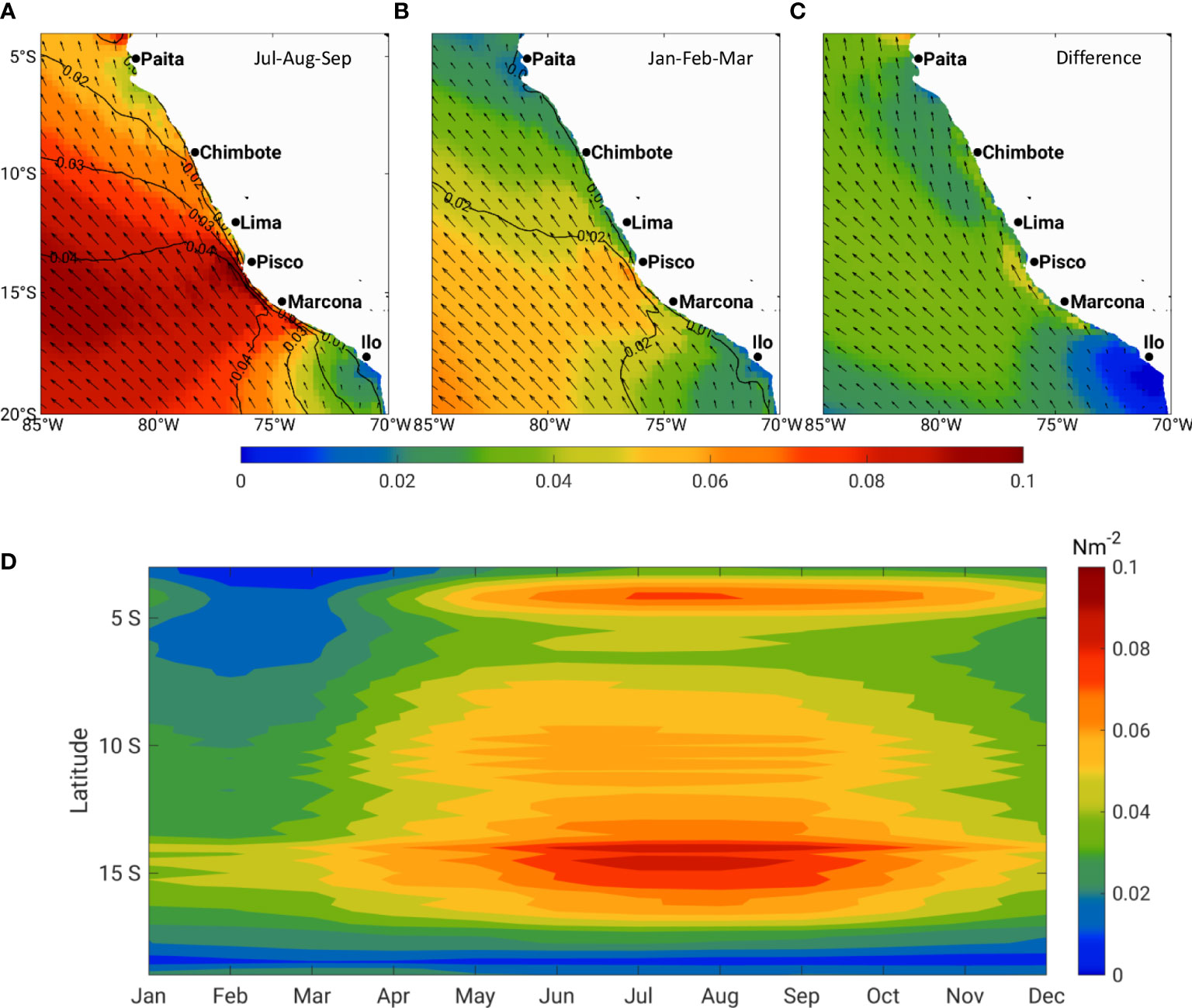
Figure 1 Mean τ (color shaded, N/m²) and direction (arrows, every third vector shown) and corresponding variability in terms of standard deviation (isolines) for (A) winter (July–September), (B) summer (January–March), and (C) difference between winter and summer, calculated using ERA5 wind over 1950–2019. Hovmöller diagram of the annual cycle of alongshore wind stress across the PUS (D). The alongshore wind stress is obtained over the first baroclinic Rossby radius distance from the coastline.

The results of Sydeman et al. (2014) support Bakun’s hypothesis by performing a meta-analysis of the results of various studies on the upwelling-favorable winds over EBUSs. They synthesized the results of 22 published studies in the period of 1990–2012, and their result confirms Bakun’s hypothesis in the Humboldt current system. This was supported by both observational and simulated data.

Most recently, Rykaczewski et al. (2015), using the result of 21 models, demonstrated that projected changes in upwelling-favorable winds are not exclusively due to the enhanced surface temperature contrast between the land and adjacent ocean. They suggested an alternate hypothesis; anthropogenic changes in the intensity of upwelling-favorable winds will be associated with shifts in the seasonal development and geographic positioning of the four major atmospheric high-pressure systems.

At the same time, the proximity of the PUS to the Eastern Pacific and its dominant modes of climate variability (i.e., ENSO and IPO) may hinder the detection of anthropogenic climate change signals. ENSO cycles are semi-regular with a periodicity of 3–7 years and have rapidly varying and long-lasting effects on the PUS ecosystems (Chavez et al., 2003; Taylor et al., 2008; Dewitte et al., 2012; Espinoza-Morriberon et al., 2017; Chamorro et al., 2018). The IPO is not necessarily independent of the ENSO. It shows a basin-wide horseshoe-like pattern that is virtually symmetric about the equator with 15–20 years of oscillation (Meehl and Hu, 2006; Parker et al., 2007; Ding et al., 2013; Henley et al., 2015 and Meehl et al., 2016). The IPO phase transitions have large influences on the wind field over the PUS.

The temporal and spatial variations of the wind field are largely affected by several local factors such as coastline geometry and orography, coastal breeze, atmosphere stability, and small-scale air–sea interactions (Renault et al., 2016). Overall, these factors tend to weaken the wind speed toward the coast, which is known as the wind drop-off phenomenon (Capet et al., 2004; Renault et al., 2012; Desbiolles et al., 2014, and Renault et al., 2015). The combination of mountain orography with a cape shape coastline has a large influence on the wind drop-off (Renault et al., 2015). This transitional area is approximately several 10 km wide and features a significant divergence in the offshore transport driven by the alongshore winds (Boe et al., 2011). The upwelling associated with the divergence of the offshore transport is known as Ekman pumping/suction and covers a larger area compared with the coastal upwelling. Thus, it is considered almost equally important as coastal upwelling for the regional marine ecosystem.

Understanding long-term variations and trends of the wind field, as a primary driver of the coastal upwelling, and their connections to the dominant modes of climate variability (e.g., ENSO and IPO) are of great importance for understanding historical changes in the PUS. So far, there have been attempts to study the PUS utilizing modeling and observational data analysis on seasonal to decadal timescales. However, given the systematic biases in the models and lack of long-term observation-based data sets with sufficiently high resolution, the model’s results on a multi-decadal timescale are subject to large uncertainty.

This study aims to analyze the wind stress field as the primary atmospheric forcing for upwelling across the PUS using 70 years of wind data provided by the European Centre for Medium-Range Weather Forecasts (ECMWF). We put special emphasis on the impacts of the IPO and the ENSO as primary modes of regional climate variability. We additionally investigate SST and the surface wind field co-variabilities across the region. In addition, we provide a detailed overview of the mean state, the seasonal cycle, and the long-term trends of the surface winds, which are of great importance for marine ecosystem communities.

The paper is organized as follows: materials and methods are described in Section 3. Section 4 presents the results, and Section 5 is dedicated to discussions and conclusions.

2 Materials and methods

2.1 Data

Among other available reanalysis products, the ERA5 product is used mainly due to its spatial resolution (0.25°×0.25°) and extended temporal coverage (1950–2020; Hersbach et al., 2020). The ERA5 surface level wind field and sea surface temperature (SST) products for the period of 1950–2019 are used. The data sets consist of two major reanalysis periods. Over 1950–1978, it was reconstructed from the assimilation of early satellite-derived data and reprocessed conventional observations (Bell et al., 2020). In contrast, vast amounts of historical observations are used after 1979, which are available a few days behind real time (Hersbach et al., 2018). ERA5 hourly products with global coverage are publicly accessible on a 0.25° × 0.25° grid. In this study, the daily mean values of wind components were computed from the hourly data.

The time series of the ENSO index (NINO 3.4) was taken from the climate prediction center of the National Oceanic and Atmospheric Administration¹ (NOAA), which was obtained from the 3-month running mean of monthly SST. The IPO index was also taken from the NOAA Physical Sciences Laboratory (PSL)².

2.2 Data analysis

The daily τ is calculated using the bulk formula:

where ρ is the air density (1.2 kg.m⁻³), $C_D^N$ is the neutral drag coefficient (Trenberth et al., 1990), and U₁₀ is the wind velocity at 10 m height above the sea surface.

Considering the impacts of wind speed on the drag coefficient is sometimes essential to accurately estimate momentum flux into the ocean over the coastal area (Brodeau et al., 2017; Bonino et al., 2022). Since the momentum flux associated with the wind is of central importance for the upwelling process in EBUSs, we used the approach of Trenberth et al. (1990), which is based on the drag coefficient varying by wind speed. This method is widely used by marine researchers.

Theory suggests that the coastal upwelling is bounded to a coastal zone in the order of the first baroclinic Rossby radius of deformation (R_i). We consider the wind over 100 km from the coastline, which is within the range of R_i across the PUS. The temporal evolution of the τ at the 100 km coastal band is calculated by zonal averaging at each latitude.

The monthly, seasonal, and annual mean of the τ and the corresponding anomaly of monthly and annual τ with the reference period of 1981–2010 are calculated. The climatological cycle of τ is calculated as well.

The anomaly of mean monthly SST is calculated using ERA5 products for 1950–2019. To estimate the wind-stress-curl-driven upwelling, we computed the curl of τ divided by the Coriolis parameter (f) as follows:

where τ_x, τ_y, f, Ω, and φ are zonal and meridional wind stresses, the Coriolis parameter, the angular speed of the earth, and the latitude, respectively. The climatological cycle for 1950–1979 and 1990–2019 is calculated. These two periods are compared to investigate the long-term trend of wind stress.

To understand the SST and surface wind field co-variability, we implement joint Empirical Orthogonal Function (EOF) analysis using ERA5 wind and SST from NOAA satellite OIv2 measurements (Kutzbach, 1967; Reynolds et al., 2007). Before conducting the EOF analysis, the climatological annual cycle was subtracted from each variable. Then, given the fact that wind and SST have different physical units and scales, we normalized them with the areal average of the standard deviation of monthly anomalies over the entire domain (85°W–70°W, 20°S–2°S). In this way, the EOF modes and their principal components (PCs) can be interpreted as the co-variability of the normalized surface wind field and SST in space and time, respectively.

3 Results

Here, we discuss the long-term mean, seasonal cycle, and interannual variability of wind stress (speed) off Peru. We also address the impacts of dominant modes of regional climate variability on the wind field. We discuss also the SST-wind stress co-variability and the long-term trend of the wind.

3.1 Long-term mean

The long-term mean and variability of wind stress (τ) are shown in Figure 2. The variability is expressed as the standard deviation of daily mean wind stress. A distinct maximum τ of approximately 0.08 N/m² is observed off Pisco, which is reduced seaward. The strong τ off Pisco–Marcona is attributed to the local effect of coastal geometry and headland. The τ shows a high variation in the Pisco–Marcona area with a standard deviation of approximately 0.03 N/m². The variability is reduced across the northern and southern coasts.

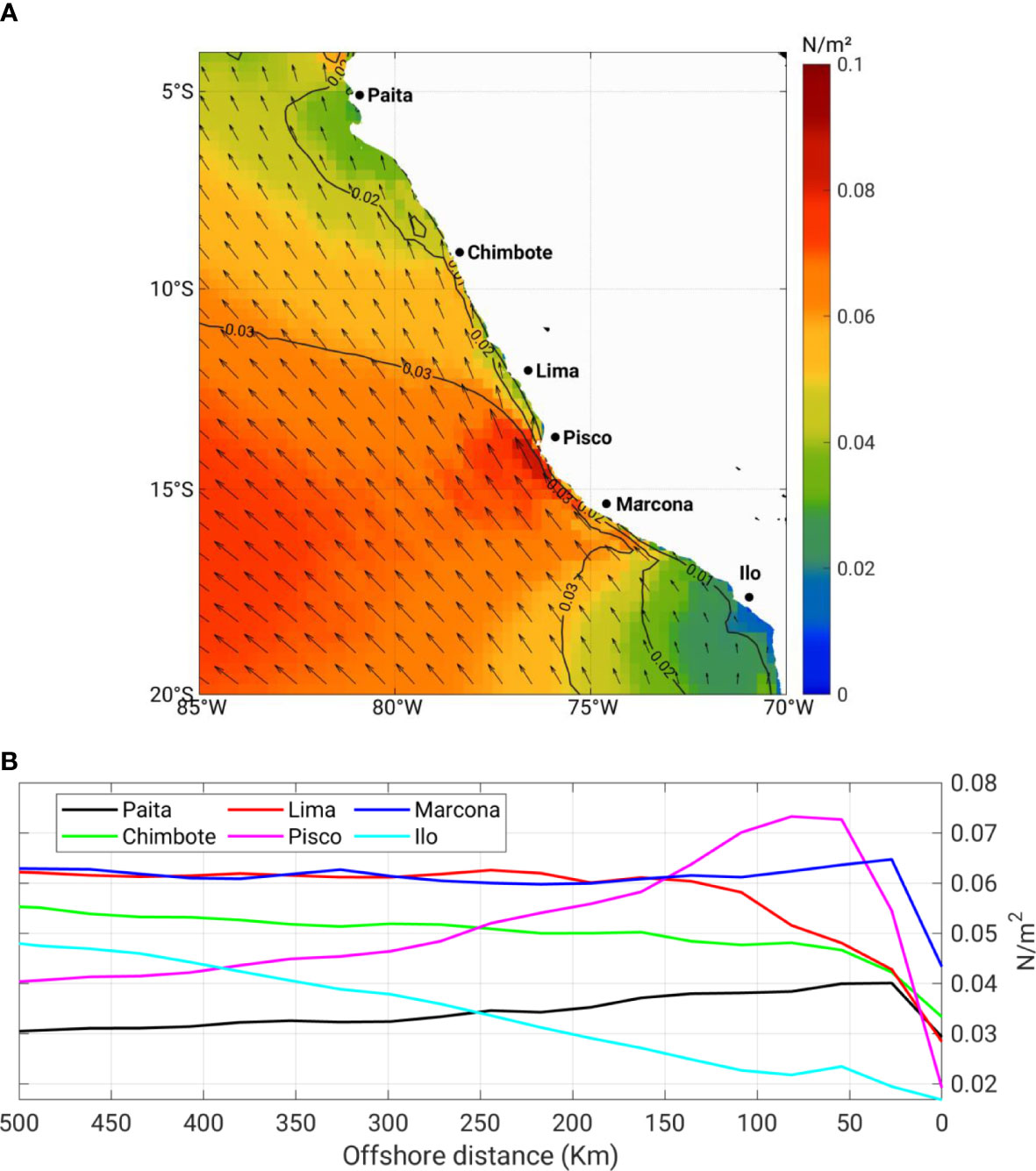
Figure 2 (A) Mean surface τ (color shading; N/m²), direction (arrows, every third vector shown), and its variability (contours; N/m²) across the Peruvian upwelling system. The variability was computed as the standard deviation of daily mean values. (B) Zonal profiles of the long-term mean τ_y for different upwelling cells across the PUS. The curves were obtained from the meridional average over a 1.0° band from the coastline to 500 km offshore distance in a zonal direction.

The alongshore component of τ shows a large variation in seaward (i.e., zonal) direction across different cells (Figure 2B). Due to the headland effect of the coastline, there is a strong wind close to the coastline of the Pisco and Marcona cells, with a steep reduction toward the land. The wind off Paita shares several similarities with that off Pisco but with a smaller magnitude. This may come down to the similar orographic and headland pattern in these two upwelling cells. Unlike the central and northern portions of the HUS, τ profile shows a stepwise enhancement with the coastal distance in the sector south of Marcona.

3.2 Seasonality

In austral summer (January–March) concurrent with the southernmost position of the intertropical convergence zone, τ experiences its seasonal minimum in the entire PUS with values of approximately 0.02–0.05 Nm⁻² in the coastal band. The standard deviation is almost uniform, approximately 0.01–0.02 Nm^-2 in the coastal area and enhanced seaward (Figure 1). The τ is more intensified in the austral autumn (April–June) and reaches the seasonal maximum in winter (July–September). Except in the southernmost portion of the HUS, the intensity of τ exceeds 0.04 Nm⁻² over the entire region in winter. It reaches approximately 0.1 Nm⁻² in the Pisco and Marcona cells. A positive seaward gradient in the τ is evident near the coast, which is more pronounced at the Pisco and Marcona. The offshore gradient becomes steeper in the Austral winter. It is important to highlight the fact that the presence of distinct maximum τ off the Pisco and Marcona cells persists throughout the year.

The annual cycle of the alongshore τ over the coastal zones with a width of R_i shows a high seasonal variation with a seasonal maximum in Austral winter (July–September) and a seasonal minimum in Austral summer (January–March). The seasonal pattern shows a non-uniform geographical distribution with a strong seasonal peak off Pisco–Marcona (13°–16°S) diminishing north- and southward (Figure 1).

3.3 ENSO events

As mentioned in previous studies (Chavez et al., 2003; Taylor et al., 2008; Dewitte et al., 2012; Espinoza-Morriberon et al., 2017; Chamorro et al., 2018), the Pacific El Niño and La Niña events exert profound impacts on the wind field in the HUS. The mean τ during El Niño and La Niña events in 1950–2019 is calculated using monthly mean and plotted in Figure 3. The criterion for selecting El Niño and La Niña events is the Nino3.4 SST anomalies. When the SST anomaly is higher (cooler) than >0.5°C and persistent for longer than 5 consecutive months, it is considered El Niño (La Niña). During the El Niño, the magnitude of τ shows higher values concerning the long-term mean, particularly along the coastal area, with a maximum of ~0.09 Nm⁻² in the Pisco upwelling cell (Figures 3A, C). On the contrary, the La Niña events are associated with reduced τ mainly in the central and northern parts (Figures 3B, D). The higher τ during the El Niño does not mean stronger upwelling and productivity. The deeper thermocline and thicker warmer water cause weaker upwelling and less nutrients and consequently lower primary production. On the contrary, during La Niña, the thermocline is shallower concerning normal conditions, which causes more nutrient supply to surface waters and higher primary production.

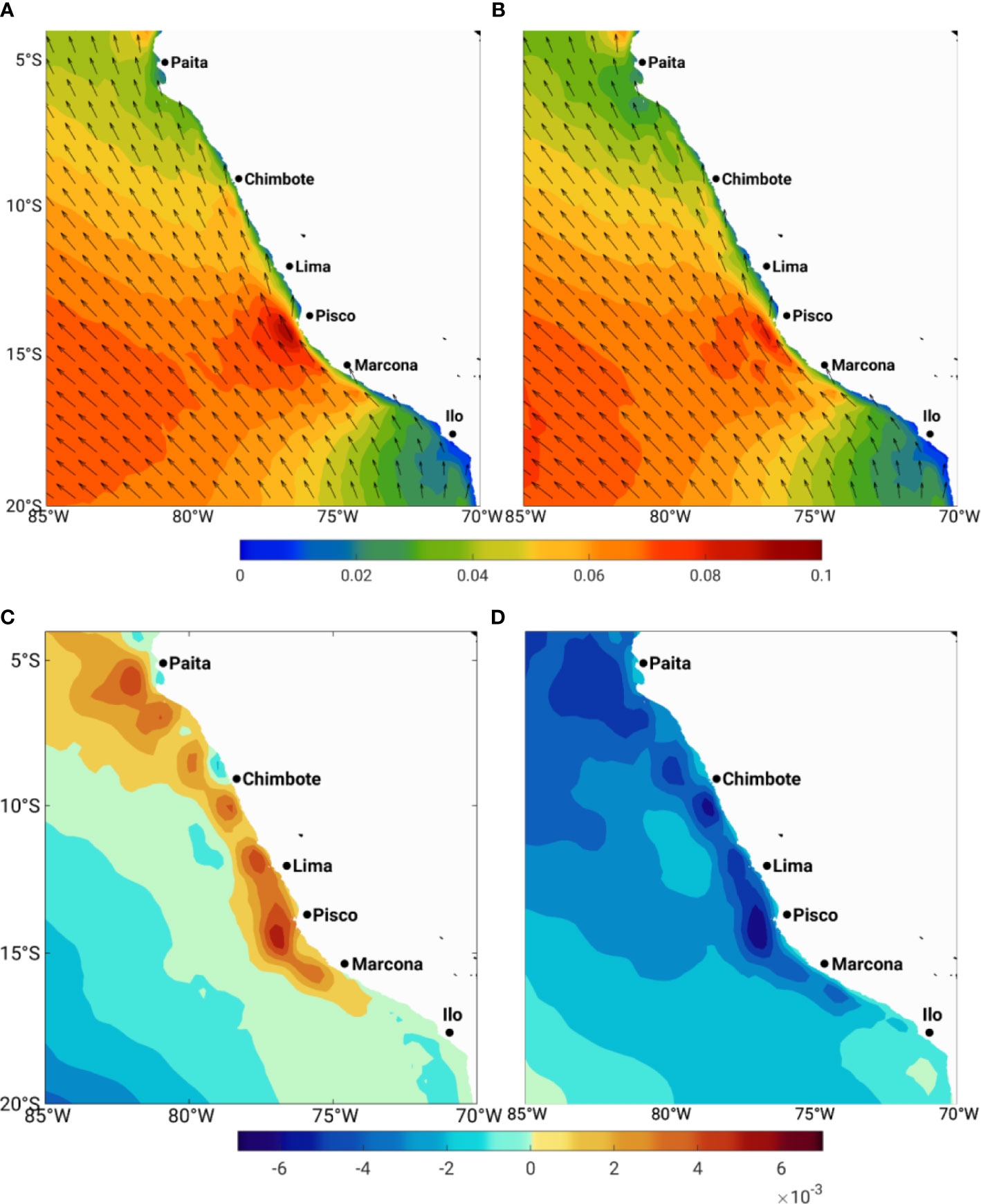
Figure 3 Mean τ (N/m²) for El Niño and direction (arrows, every third vector shown) (A) and its difference from the mean state (C), and La Niña and direction (arrows, every third vector shown) (B) and its difference from mean state (D) off Peru. It is obtained from ERA5 wind data from 1950 to 2019.

3.4 Coastal domain

The time evolution of yearly mean alongshore τ anomalies over the 100-km coastal band is displayed in Figure 4. It shows fluctuations on interannual to decadal time scales. A year-to-year oscillation with more signatures in the central and southern sectors of the PUS is obvious, which is likely associated with the ENSO events. Robust positive (equatorward) anomalies in 1983, 1995, 1998, 2002, 2010, and 2015 coincide with pronounced El Niño events. Moreover, a transition from negative to positive anomalies was evident around 1997. A mirror-like pattern is observed around 2015. However, the center of large positive and negative anomalies during these two events does not appear at the same location. It might be connected to the asymmetric behavior of the ENSO and the IPO. During 1997–2015, the anomaly of τ is positive over the entire coastal domain. This situation is not only dominated in the coastal domain but also appears in the offshore area (not shown here). In addition, there is a relatively weak decadal negative anomaly period for 1972–1983, which is followed by another negative in 1984–1995 after a positive signal in 1983–1984. These systematic decadal changes resemble the transition phase of the IPO.

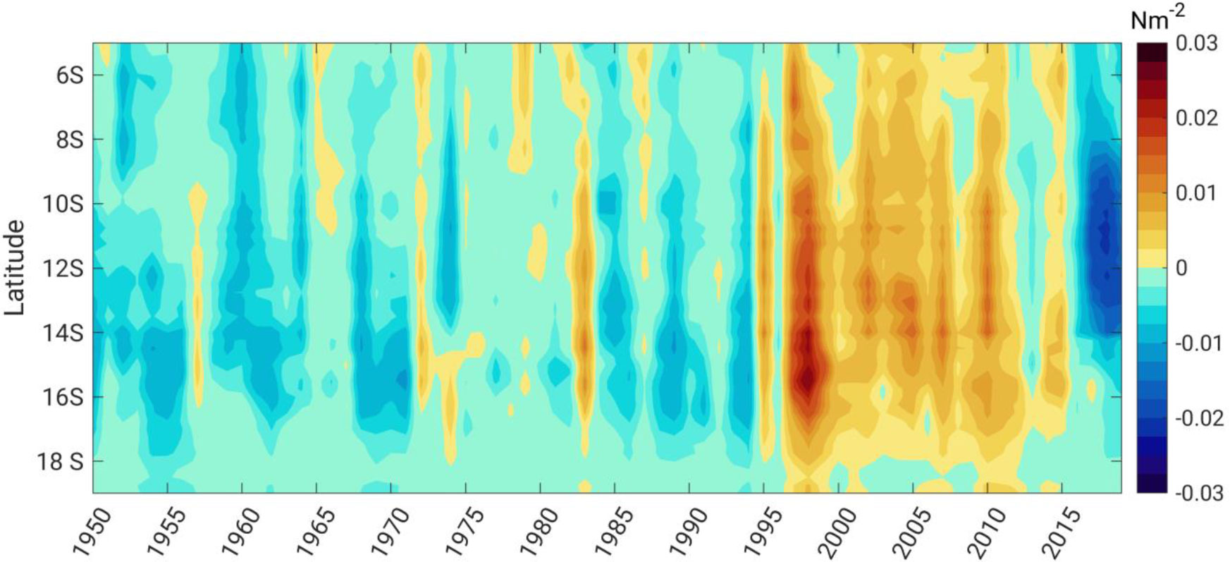
Figure 4 Hovmöller diagram of the yearly mean of alongshore wind stress anomaly over the 100 km coastal band across the PUS. Note that the long-term mean was subtracted before computing the yearly mean.

We applied low pass filters (1- and 5-year running average) to the time series of monthly mean alongshore τ anomalies over the coastal stripe of the Peruvian coast (5S–18S) (Figure 5). The presence of fluctuations in interannual and interdecadal timescales in the time series is evident. The interannual fluctuation of the wind stress is in phase with ENSO cycles. The same is true for the long-term fluctuations of τ and the IPO cycle, but they are out of phase. The pronounced shift from negative to positive τ anomalies in 1996 and from positive to negative in 2015 is apparent in the time series, which is in good agreement with IPO phase transitions. The negative phase of the IPO, which is a basin-wide La Niña-like pattern, is observed concurrent with the positive wind stress anomalies. This is also true for the period from 1975 to 2019.

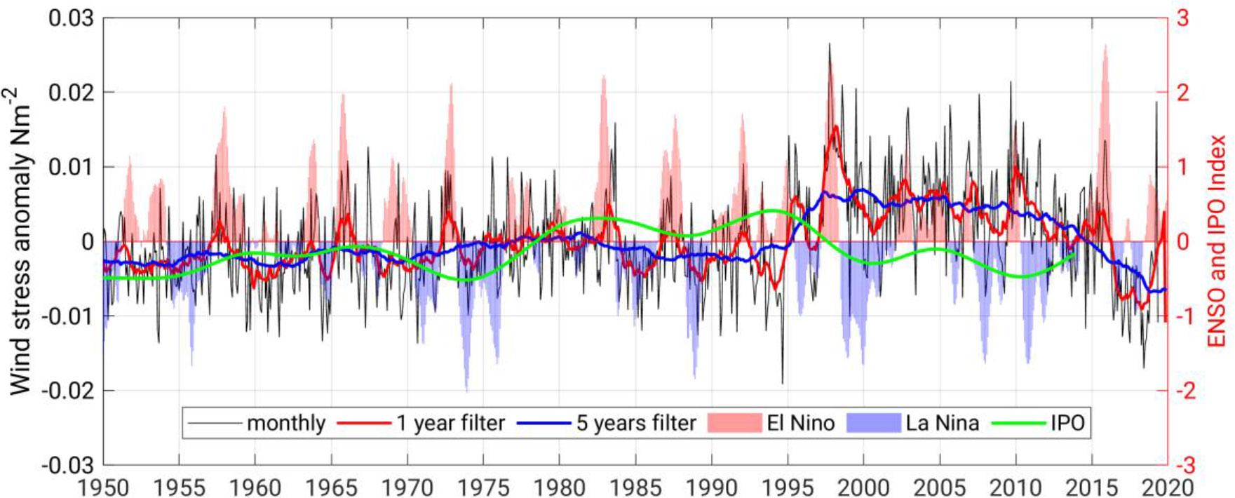
Figure 5 Anomaly of mean monthly (black curves), 1-year (red curve), and 5-year (blue curve) running means of alongshore wind stress across the PUS (coastal stripe over 5S–18S). The time series of the IPO index is shown by green lines. Red and blue shadings indicate El Niño and La Niña events, respectively. Note that alongshore wind stress is averaged over a coastal distance of 100 km.

The linear correlation between the time series is also examined. The correlation coefficient of monthly τ and ENSO is approximately 0.28. Considering the entire period, the correlation coefficient of monthly τ and the IPO is not statistically significant. Therefore, the time series of IPO is divided into two periods; the first period is 1950–1978, and the second period is 1979–2015. The monthly τ anomalies show a small correlation of approximately 0.09 with the first period (1950–1978). In contrast, it is anti-correlated with the second period of IPO with a correlation coefficient of approximately −0.36. The 1-year filtered data have correlation coefficients of 0.27, 0.22, and −0.57 with ENSO and with the first and second periods of IPO, respectively. The 5-year filtered data show a high negative correlation coefficient with the second period of IPO as −0.73 and 0.32 with the first period of IPO (Table 1).

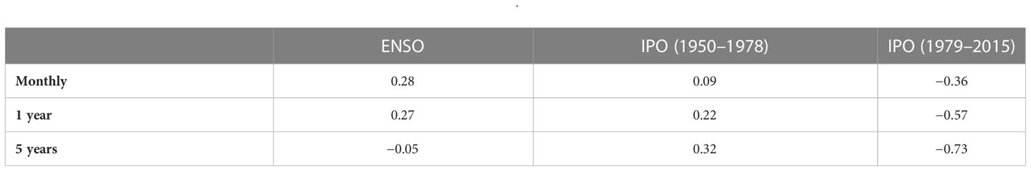
Table 1 Correlation coefficients between time series presented in Figure 5.

To investigate the co-variation of the rotation wind stress and SST, the cross-correlation between monthly mean anomalies of SST and curl(τ)/f is examined (Figure 6). Since the dominant driver of upwelling near the coastal band of about the first baroclinic Rossby radius of deformation is the alongshore wind-driven upwelling (Bordbar et al., 2021), we do not show the correlation over the coastal zone. The higher value is obtained with curl(τ)/f leading by 1 month. The curl(τ)/f is proportional to the offshore vertical transport. Since the main driver of upwelling near the coast is along-shore wind-driven upwelling, we only discuss the aforementioned correlation offshore (>100km off coast). It is shown that the curl(τ)/f, and SST is widely anti-correlated: implying that the enhanced curl(τ)/f is very likely followed by SST cooling. A higher correlation is observed off the upwelling cells.

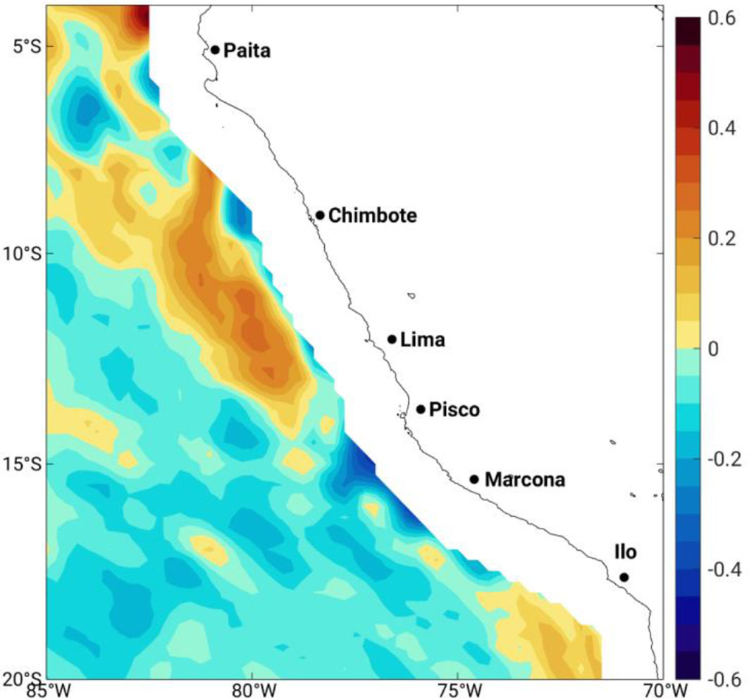
Figure 6 Spatial pattern of the correlation coefficient between anomalies of monthly SST and curl(τ)/f. Please note that curl(τ)/f is leading SST by 1 month.

To understand the coherent variation in surface wind and SST variability, we conducted joint wind-SST EOF analysis using the monthly SST and wind anomalies (Figure 7). In this way, the co-variability of the surface wind and SST is reflected in the spatial pattern of the EOFs. Here, we show the results of our analysis for the first four EOF modes. The remaining modes appear less significant, with the percentage of explained variability typically<3.5%. The first mode (Figure 7A) explains more than 47% of the total variability. It features northwesterly/southeasterly anomalies in the surface wind, almost the same magnitude over the entire domain. The pronounced phase transition occurred around 1995 (Figure 7E), which was nearly coincident with the phase transition of the IPO. The correlation of PC1 with the IPO is approximately 0.42. However, the SST variation in this mode is small relative to that for the wind. The second and third modes seem to be related to the ENSO fluctuations and explain more than 28% of the total variability (Figures 7B, C). The corresponding PCs display fluctuations on interannual timescales (Figures 7F, G). The pronounced peaks in 1982–1983, 1987–1988, 1997–1998, and 2015–2016 in the second PC reminds the strong El Niño events. The correlation between the second PC and Nino3.4 index is approximately 0.60. The wind anomaly associated with the second mode is small compared with other modes. The warming during the El Niño-like phase is associated with the local deepening of the thermocline and elevated sea level driven by upper ocean heat content transported from the western tropical Pacific. Thus, the local wind plays rather a minor role in this mode. However, the third mode, which seems to be ENSO related, suggests a cooling associated with equatorial winds with more signature near the coast. A close connection between the spatial pattern of SST and wind is viewed in the fourth mode. However, this mode explains only 4.3% of the total variability.

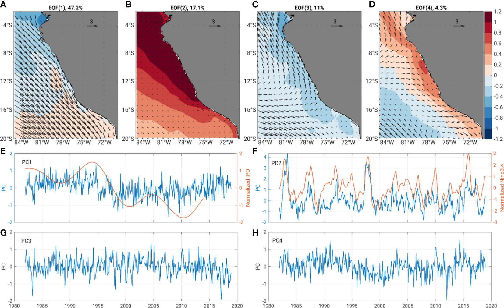
Figure 7 The results of joint wind-SST EOF analysis over the PUS. The spatial patterns of EOF1-4 are shown in panel (A–D). The explained variability by each EOF is shown on the top of panels (A–D). The time series of the corresponding PCs are displayed in panel (E–H). The red curves in panels (E, F) represent the normalized time series of the IPO and Niño3.4 index. We used the monthly mean SST and surface wind from OISST and ERA5 data sets from 1982 to 2019, respectively. The climatological monthly mean values were subtracted before computing the EOFs.

To investigate the influence of El Niño and La Niña on the meridional wind stress, we regressed the monthly mean wind stress onto the monthly ENSO index. It shows higher coefficients off the upwelling cells with a maximum of 0.42 in the Pisco area (Figure 8). This coefficient is particularly larger off the Pisco cell. We additionally applied the regression for the El Niño and La Niña episodes separately. The coefficients are 0.61 and 0.28 for El Niño and La Niña, respectively. The El Niño and La Niña events are decomposed based on the SST anomalies over the Nino3.4 index. The anomalies larger (smaller) than 1.0 (−1.0) are considered El Niño (La Niña) events. During El Niño, wind over the coastal zones is intensified, which is more pronounced off Pisco, Lima, Chimbote, and Paita. The weakening of the wind over the coastal zone is evident during La Niña. However, the impact of La Niña appears to be not mirror-like of El Niño. For example, wind over the central and southern portion of the PUS appears to be anti-correlated with the Nino3.4 SST during La Niña. In contrast, the wind over these sectors is marginally affected by the Nino3.4 SST during El Niño. It reminds the asymmetric features of ENSO cycles. Overall, coastal upwelling is more affected during warm (i.e., El Niño) than cold (i.e., La Niña) episodes.

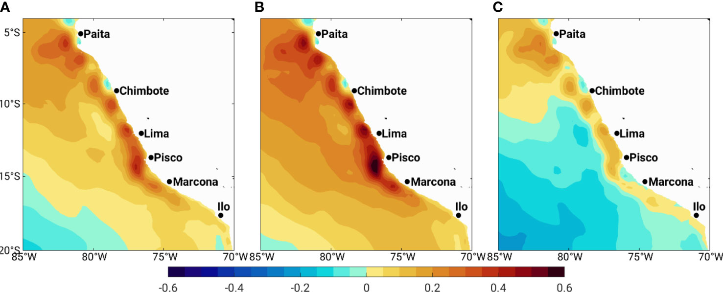
Figure 8 Spatial pattern of the regression coefficient (N/m²C) between meridional wind stress and ENSO (A), El Niño (B), and La Niña (C) events. In the regression, the predicted parameter is wind stress.

3.5 Long-term trend

The long-term trend of meridional wind stress over the coastal domain and offshore areas shows a positive trend. The climatological mean over the periods of 1950–1979 and 1990–2019 and the difference between the two periods are shown in Figure 9. The distribution of trend (Figure 9C) shows positive values in almost all areas except the northernmost of the domain (above 5°S) with the maximum value in the Pisco area. The long-term wind intensification across the PUS can be largely attributed to the strengthening and southwest migration of the Pacific Subtropical Anticyclone (Ancapichún and Garcés-Vargas, 2015). Detailed information on the connection between the Pacific subtropical anticyclone and wind-driven upwelling across the PUS would be very beneficial for improving regional decadal prediction, which is beyond the current study.

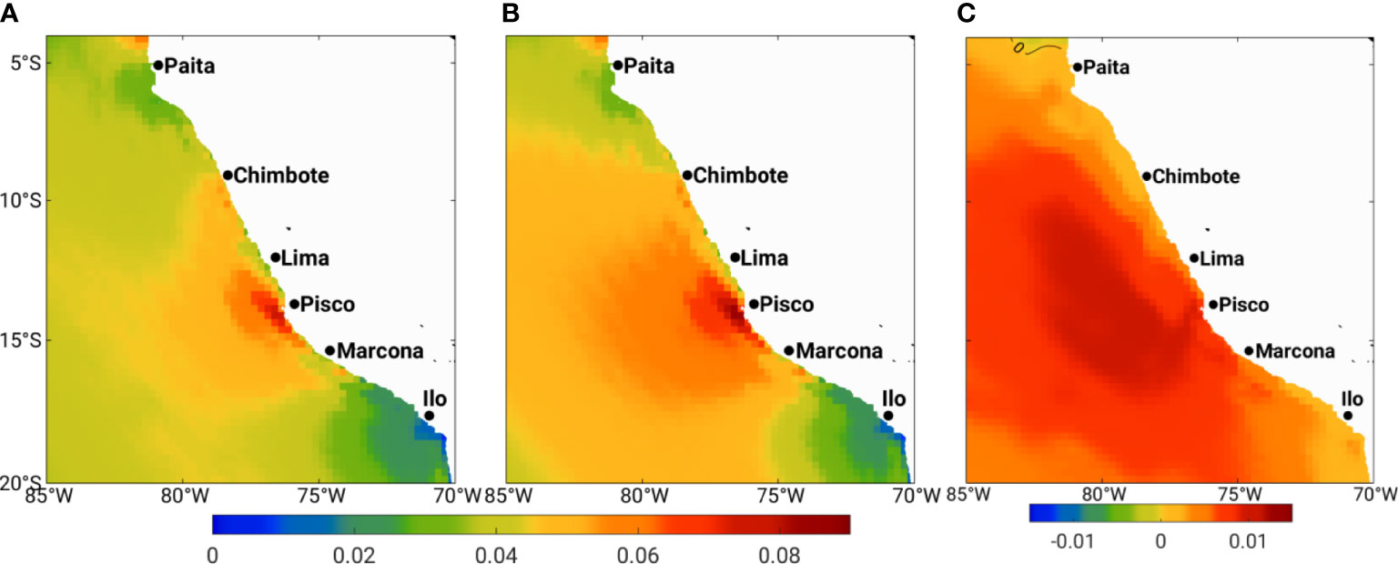
Figure 9 The climatology of the meridional wind stress (N/m²) over the entire study area for the period of 1950–1979 (A), 1990–2019 (B), and the difference between two periods, 1990–2019 minus 1950–1979 (C), calculated using ERA5 wind data. The isoline on (C) shows zero wind stress.

In addition, the trend of the meridional wind stress over the coastal zone is calculated. First, the linear trend for the austral winter (July–September) wind stress over the coastal band (100 km) is computed. Given the phase locking of the ENSO cycle, the winter-time wind stress is slightly affected by the ENSO-related oscillations. This shows a positive trend in the entire coastal domain with higher values off the Pisco upwelling cell (Figure 10). The meridional wind stress shows a long-term upward trend of approximately ~0.001 Nm⁻² per decade. Second, the impact of ENSO is subtracted from the monthly wind stress using linear regression. Again, the result shows an upward trend, which is comparable with the previous trend.

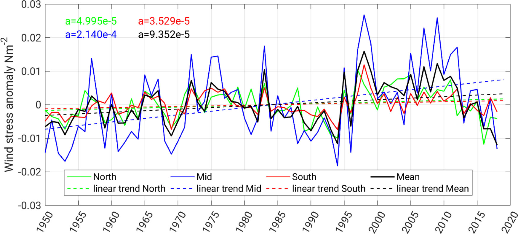
Figure 10 The yearly mean anomaly of the meridional wind stress for winter (July–September) over the coastal 100-km domain. The red, blue, green, and black lines represent the wind stress over the northern, central, and southern portions of the domain, respectively. Black lines indicate the wind averaged over the entire domain. The dashed lines are the linear trend. The linear trend coefficients (Nm⁻²/year) are given with similar colors.

4 Discussions and conclusions

Using the ERA5 reanalysis, we assessed wind stress’ temporal and spatial variations in the Peruvian Upwelling System (PUS) over the last seven decades. The long-term mean and seasonal cycle of wind stress were shown and discussed. On the long-term average, wind over the central PUS is intensified, which can be attributed to the headland effect. In general, the coastal and offshore winds over the southern portion of the PUS undergo more variability than the northern portion. The exception is the wind off the Paita upwelling cell in the northern portion of the PUS, which features a large variation. ENSO cycles exert profound impacts on the wind across the entire PUS. El Niño episodes feature intensified winds with more signature off Pisco. Interestingly, the wind anomaly during La Niña is not the opposite of that for El Niño, highlighting the asymmetric feature of the ENSO cycle. Our findings show a semi-regular variation on the decadal timescale and beyond, closely followed by the Interdecadal Pacific Oscillation cycles. For example, the transition of IPO from the negative to a positive phase in the late 1970s was concurrent with the weakening of the winds across the PUS. In contrast, the IPO phase reversal in the late 1990s was accompanied by the strengthening the PUS winds, which lasted for almost two decades. However, the ERA5 time span (~70 years) is insufficient to discuss the detailed structure of wind anomaly associated with the IPO. Our analysis indicates a long-term intensification of wind over the entire PUS. This intensification is more pronounced in the upwelling zones, consistent with previous studies, and very likely associated with the intensification of the South Pacific Anticyclone.

In addition, we conducted the joint wind-SST Empirical Orthogonal Function. The first mode is on a decadal timescale, explains more than 40% of variability, and is more related to the wind than SST. The wind anomaly associated with this mode is directed northwesterly/southeasterly and almost uniform across the entire domain. The associated principal component (PC) fluctuations are almost in phase with the IPO. This further highlights the teleconnection between climate variability over the extratropical Pacific and wind variability across the BUS. The second and third modes and their PCs share many similarities with ENSO cycles. In general, local wind variability tends to be more affected by the IPO, whereas the SST appears more related to the ENSO. The wind anomaly during El Niño is equatorward. However, the SST anomaly is pronounced and negative. It is likely due to the deepening of the thermocline and eastward propagation of upper ocean heat content during El Niño.

Data availability statement

The original contributions presented in the study are included in the article/supplementary material. Further inquiries can be directed to the corresponding author.

Author contributions

VM is the head of the project and designed the study. SY performed the whole data analysis and all authors contributed to the writing and revision. All authors contributed to the article and approved the submitted version.

Acknowledgments

This study was conducted within the frame of the CUSCO project sponsored by the Federal Ministry of Education and Research (BMBF) with the reference number CUSCO-03F0813E. The ERA5 data sets were obtained from ECMWF. We appreciate the reviewer for his/her constructive comments and suggestions, which helped to improve the manuscript.

Conflict of interest

The authors declare that the research was conducted in the absence of any commercial or financial relationships that could be construed as a potential conflict of interest.

Publisher’s note

All claims expressed in this article are solely those of the authors and do not necessarily represent those of their affiliated organizations, or those of the publisher, the editors and the reviewers. Any product that may be evaluated in this article, or claim that may be made by its manufacturer, is not guaranteed or endorsed by the publisher.

Footnotes

1. ^ https://origin.cpc.ncep.noaa.gov/products/analysis_monitoring/ensostuff/ONI_v5.php
2. ^ https://psl.noaa.gov/data/timeseries/IPOTPI/

References

Ancapichún S., Garcés-Vargas J. (2015). Variability of the southeast pacific subtropical anticyclone and its impact on sea surface temperature off north-central Chile. Cienc. Marinas 41 (1), 1–20. doi: 10.7773/cm.v41i1.2338
Bakun A. (1990). Global climate change and intensification of coastal ocean upwelling. Science 247, 198–201. doi: 10.1126/science.247.4939.198
Bakun A., Black B. A., Bograd S. J., García-Reyes M., Miller A. J., Rykaczewski R. R., et al. (2015). Anticipated effects of climate change on coastal upwelling ecosystems. Curr. Clim. Change Rep. 1, 85–93. doi: 10.1007/s40641-015-0008-4
Barros V.B., C. B. Field, D. J. Dokken, M. D. Mastrandrea, K. J. Mach, T. E. Bilir, et al(2014). Climate change 2014: impacts, adaptation, and vulnerability. part b: regional aspects. Contribution Working Group II to Fifth Assess. Rep. ofthe Intergovernmental Panel Climate Change (Cambridge; New York, NY), 688.
Bell B., Hersbach H., Berrisford P., Dahlgren P., Horányi A., Muñoz Sabater J., et al. (2020) ERA5 hourly data on single levels from 1950 to 1978 (preliminary version) (Copernicus Climate Change Service (C3S) Climate Data Store (CDS). Available at: https://cds.climate.copernicus-climate.eu/cdsapp#!/dataset/reanalysis-era5-single-levels-preliminary-back-extension?tab=overview (Accessed 25-01-2021).
Belmadani A., Echevin V., Codron F., Takahashi K., Junquas C. (2013). What dynamics drive future wind scenarios for coastal upwelling off Peru and Chile? Clim. Dyn 43, 1893–1914. doi: 10.1007/s00382-013-2015-2
Boe J., Hall A., Colas F., McWilliams J., Qu X., Kurian J., et al. (2011). What shapes mesoscale wind anomalies in coastal upwelling zones? Clim. Dyn. 36, 2037–2049. doi: 10.1007/s00382-011-1058-5
Bonino G., Iovino D., Brodeau L., Masina S. (2022). The bulk parameterizations of turbulent air-sea fluxes in NEMO4: the origin of Sea surface temperature differences in a global model study. Geoscientific Model. Dev. Discussions, 1–20.
Bordbar M. H., Mohrholz V., Schmidt M. (2021). The relation of wind-driven coastal and offshore upwelling in the benguela upwelling system. J. Phys. Oceanogr. 51, 3117–3133. doi: 10.1175/JPO-D-20-0297.1
Brodeau L., Barnier B., Gulev S. K., Woods C. (2017). Climatologically significant effects of some approximations in the bulk parameterizations of turbulent air–sea fluxes. J. Phys. Oceanography 47 (1), 5–28.
Capet X. J., Marchesiello P., McWilliams J. C. (2004). Upwelling response to coastal wind profiles. Geophys. Res. Lett. 3, L13311. doi: 10.1029/2004GL020123
Chamorro A., Echevin V., Colas F., Oerder V., Tam J., Quispe-Ccalluari C. (2018). Mechanisms of the intensification of the upwelling-favorable winds during El niño 1997–1998 in the Peruvian upwelling system. Climate Dynamics 51, 3717–3733. doi: 10.1007/s00382-018-4106-6
Chavez F. P., Messié M. (2009). A comparison of eastern boundary upwelling ecosystems. Prog. Oceanogr. 83, 80–96. doi: 10.1016/j.pocean.2009.07.032
Chavez F. P., Ryan J., Lluch-Cota S., Miguel Ñiquen C. (2003). From anchovies to sardines and back: multidecadal change in the pacific ocean. Science 299 (5604), 217–221. doi: 10.1126/science.1075880.
Desbiolles F., Blanke B., Bentamy A., Grima N. (2014). Origin of fine-scale wind stress curl structures in the benguela and canary upwelling systems. J. Geophys. Res. 119 (11), 7931–7948. doi: 10.1002/2014JC010015
Dewitte B., Vazquez-Cuervo J., Goubanova K., Illig S., Takahashi K., Cambon G., et al. (2012). Change in El nino flavours over 1958-2008: implications for the long-term trend of the upwelling off Peru. Deep-Sea Res. Pt. II 77–80, 143–156. doi: 10.1016/j.dsr2.2012.04.011
Ding H., Greatbatch R., Latif M., Park W., Gerdes R. (2013). Hindcast of the 1976/77 and 1998/99 climate shifts in the pacific. J. Climate 26, 7650–7661. doi: 10.1175/JCLI-D-12-00626.1
Echevin V., Colas F., Chaigneau A., Penven P. (2011). Sensitivity of the northern Humboldt current system nearshore modeled circulation to initial and boundary conditions. J. Geophys. Res. 116, C07002. doi: 10.1029/2010JC006684
Espinoza-Morriberon D., Echevin V., Colas F., Tam J., Ledesma J., Vasquez L., et al. (2017). Impacts of El niño events on the Peruvian upwelling system productivity. J. Geophys. Res. Oceans 122, 5423–5444. doi: 10.1002/2016JC012439
García-Reyes M., Sydeman W. J., Schoeman D. S., Rykaczewski R. R., Black B. A., Smit A. J., et al. (2015). Under pressure: climate change, upwelling, and Eastern boundary upwelling ecosystems. Front. Mar. Sci. 2. doi: 10.3389/fmars.2015.00109
Guillen O. (1983). Condiciones oceanognificas y sus fluctuaciones en el pacifico sur oriental. FAO Fish Rep. 3, 607–658.
Henley B., Gergis J., Karoly D., Power S., Kennedy J., Folland C. (2015). A tripole index for the interdecadal pacific oscillation. Climate Dynamics 45, 3077–3090. doi: 10.1007/s00382-015-2525-1
Hersbach H., Bell B., Berrisford P., Biavati G., Horányi A., Muñoz Sabater J., et al. (2018) ERA5 hourly data on single levels from 1979 to present (Copernicus Climate Change Service (C3S) Climate Data Store (CDS) (Accessed 11.09.2019).
Hersbach H., Bell B., Berrisford P., Hirahara S., Horányi A., Muñoz-Sabater J., et al. (2020). The ERA5 global reanalysis. Q. J. R. Meteorol. Soc 146 (2020), 1999–2049. doi: 10.1002/qj.3803
Jacox M. G., Moore A. M., Edwards C. A., Fiechter J. (2014). Spatially resolved upwelling in the California current system and its connections to climate variability. Geophys. Res. Lett. 41, 3189–3196. doi: 10.1002/2014GL059589
Kutzbach J. E. (1967). Empirical eigenvectors of sea-level pressure, surface temperature and precipitation complexes over north America. J. Appl. Meteorol. Climatol. 6 (5), 791–802. doi: 10.1175/1520-0450(1967)006<0791:EEOSLP>2.0.CO;2
Meehl G. A., Hu A. (2006). Megadroughts in the Indian monsoon region and southwest north America and a mechanism for associated multi-decadal pacific sea surface temperature anomalies. J. Climate 19, 1605–1623. doi: 10.1175/JCLI3675.1
Meehl G., Hu A., Teng H. (2016). Initialized decadal prediction for transition to positive phase of the interdecadal pacific oscillation. Nat. Commun. 7, 11718. doi: 10.1038/ncomms11718
Montecinos A., Purca S., Pizarro O. (2003). Interannual-to-interdecadal sea surface temperature variability along the western coast of south America. Geophys. Res. Lett. 30, 1570. doi: 10.1029/2003GL017345
Narayan N., Paul A., Mulitza S., Schulz M. (2010). Trends in coastal upwelling intensity during the late 20th century. Ocean Sci. 6, 815–823. doi: 10.5194/os-6-815-2010
Oyarzún D., Brierley C. M. (2019). The future of coastal upwelling in the Humboldt current from model projections. Clim. Dyn 52, 599–615. doi: 10.1007/s00382-018-4158-7
Parker D., Folland C., Scaife A., Knight J., Colman A., Baines P., et al. (2007). Decadal to multidecadal variability and the climate change background. J. Geophys. Res. 112, D18115. doi: 10.1029/2007JD008411
Renault L., Deutsch C., McWilliams J. C., Frenzel H., Liang J. H., Colas F. (2016). Partial decoupling of primary productivity from upwelling in the California current system. Nat. Geosci. 9 (7), 505–508. doi: 10.1038/ngeo2722
Renault L., Dewitte B., Marchesiello P., Illig S., Echevin V., Cambon G., et al. (2012). Upwelling response to atmospheric coastal jets off central Chile: a modeling study of the October 2000 event. J. Geophys. Res. 117, C02030. doi: 10.1029/2011JC007446
Renault L., Hall A., McWilliams J. C. (2015). Orographic shaping of US West coast wind profiles during the upwelling season. Clim. Dyn. 46, 273–289. doi: 10.1007/s00382-015-2583-4
Reynolds R. W., Smith T. M., Liu C., Chelton D. B., Casey K. S., Schlax M. G., et al. (2007). Daily high-resolution blended analyses for sea surface temperature. J. Climate 20, 5473–5496. doi: 10.1175/2007JCLI1824.1
Rykaczewski R. R., Dunne J. P., Sydeman W. J., García-Reyes M., Black B. A., Bograd S. J. (2015). Poleward displacement of coastal upwelling-favorable winds in the ocean’s eastern boundary currents through the 21st century. Geophys. Res. Lett. 42, 6424–6431. doi: 10.1002/2015GL064694
Sydeman W. J., García-Reyes M., Schoeman D., Rykaczewski R. R., Thompson S. A., Black B. A., et al. (2014). Climate change and wind intensification in coastal upwelling ecosystems. Science 345, 77–80. doi: 10.1126/science.1251635
Taboada F. G., Stock C. A., Griffies S. M., Dunne J., John J. G., Small R. J., et al. (2019). Surface winds from atmospheric reanalysis lead to contrasting oceanic forcing and coastal upwelling patterns. Ocean Modeling 133, 79–111. doi: 10.1016/j.ocemod.2018.11.003
Taylor M. H., Wolff M., Mendo J., Yamashiro C. (2008). Changes in trophic flow structure of independence bay (Peru) over an ENSO cycle. Prog. Oceanogr. 79 (2-4), 336–351. doi: 10.1016/j.pocean.2008.10.006
Trenberth K., Large W., Olson J. (1990). The mean annual cycle in global ocean wind stress. J. Phys. Oceanogr. 20, 1742–1760. doi: 10.1175/1520-0485(1990)020<1742:TMACIG>2.0.CO;2
Keywords: Humboldt Upwelling System, Eastern Boundary Upwelling Systems (EBUS), climate change, coastal alongshore winds, Interdecadal Pacific Oscillation (IPO), El Niño Southern Oscillation (ENSO)
Citation: Yari S, Mohrholz V and Bordbar MH (2023) Wind variability across the North Humboldt Upwelling System. Front. Mar. Sci. 10:1087980. doi: 10.3389/fmars.2023.1087980
Received: 02 November 2022; Accepted: 30 June 2023;
Published: 19 July 2023.
Edited by:
Francisco Machín, University of Las Palmas de Gran Canaria, SpainReviewed by:
Giulia Bonino, Foundation Euro-Mediterranean Center on Climate Change (CMCC), ItalyEduardo Zorita, Helmholtz Centre for Materials and Coastal Research (HZG), Germany
Copyright © 2023 Yari, Mohrholz and Bordbar. This is an open-access article distributed under the terms of the Creative Commons Attribution License (CC BY). The use, distribution or reproduction in other forums is permitted, provided the original author(s) and the copyright owner(s) are credited and that the original publication in this journal is cited, in accordance with accepted academic practice. No use, distribution or reproduction is permitted which does not comply with these terms.
*Correspondence: Sadegh Yari, sadegh.yari@io-warnemuende.de