Substantial Sub-Surface Chlorophyll Patch Sustained by Vertical Nutrient Fluxes in Fram Strait Observed With an Autonomous Underwater Vehicle

Highlights

– AUV allows for the observation of a phytoplankton patch associated with a front in Fram Strait.

– A frontal jet, symmetric, inertial/centrifugal as well as gravitational and shear instabilities might induce mixing at a shallow front within the surface ocean.

– Instability analyses indicate that the high chlorophyll patch is likely sustained by vertical nutrient fluxes.

Introduction

Sea ice retreat in the Arctic Ocean is dramatically changing the ocean’s light regime with drastic implications for the ecosystem. Satellite observations indicate an increase in Arctic Ocean net primary production by 30% between 1998 and 2012 (Arrigo and van Dijken, 2015) and by as much as 57% between 1998 and 2018 (Lewis et al., 2020). This is mainly attributed to increases in photosynthetically active radiation (PAR), which increases the limiting role of nutrients for primary production (Tremblay et al., 2008; Tremblay and Gagnon, 2009; Taylor et al., 2013). However, satellite vision is limited to the near-surface ocean, and cannot detect standing stocks of subsurface-chlorophyll. Model projections on the future Arctic ecosystem predict that primary production increases may occur along the Atlantic- and Pacific-water inflow pathways and along the continental slopes, where stratification weakens due to reductions in sea ice melt (Slagstad et al., 2015). These projections further indicate, that central Arctic regions away from the boundaries may not become significantly more productive. There, the effect of enhancing PAR levels is countered by increasing stratification due to enhanced ice melt and thermal warming. On a pan-Arctic scale, stratification regulates vertical mixing and nutrient fluxes into the sunlit surface layer (euphotic zone) (e.g., Doney, 2006; Randelhoff et al., 2020) and is therefore a key parameter needed to adequately project the state of the future Arctic ecosystem. Vertical mixing and other processes regulating stratification, however, occur on small scales, are not easily measured with traditional sampling methods, and are therefore not sufficiently understood. This is especially true under a changing Arctic icescape, that is characterized by increased mobility and variability (Serreze et al., 2007; Stroeve et al., 2007).

The marginal ice zone (MIZ) is becoming increasingly important under a continuously northward progressing seasonal sea ice edge. Strong and Rigor (2013) determined the MIZ to widen by 13 km decade^–1 between 1979 and 2011. Physical processes at the MIZ and their coupling to biological activity are complex and occur on small scales induced by strong gradients in water masses, light availability, surface stress, fronts, and meanders (Niebauer and Alexander, 1985; Smith et al., 1985; Engelsen et al., 2002; Perrette et al., 2011). In Fram Strait satellite-based studies found that phytoplankton growth is promoted by sea ice melt in the MIZ (seeding, stratification), while in the open ocean south of the MIZ it is governed by thermal warming (Cherkasheva et al., 2014). In a third regime, near the coast of Svalbard, a suppression of phytoplankton growth goes along with the presence of ice in early summer. Fram Strait is the major Arctic gateway, where warm inflowing Atlantic water (AW) encounters outflowing Polar water (PW) along with the south-ward sea ice export. Interactions between the swift West Spitsbergen Current, topographic irregularities, water mass gradients, sea ice and winds contribute to strong fronts and strong mesoscale activity that occur there (Hattermann et al., 2016; von Appen et al., 2016; Wekerle et al., 2017). Furthermore, a model study by Schourup-Kristensen et al. (2021) found that mesoscale processes vary on seasonal time scales and control phytoplankton growth in this region. Long-term observational efforts using oceanographic moorings are in place to monitor transports across Fram Strait (Beszczynska-Möller et al., 2012), and numerous shipboard expeditions regularly occupy Fram Strait for multi-disciplinary surveys (Nöthig et al., 2020). However, the spatial coverage needed to survey and understand mesoscale features and their multi-disciplinary impact is generally not achieved with traditional surveys. von Appen et al. (2018) surveyed a filament in Fram Strait with high-resolution CTD (conductivity temperature depth) profiles and shipboard current profilers, and were able to characterize hydrographic frontal features and their associated small-scale motion. They further found the accumulation of high chlorophyll near the center of the front in 20–30 m water depth. A biogeochemical characterization of this filament showed the strong link between plankton community structure and the physical processes at this particular feature (Fadeev et al., 2021), and underline the importance of small-scale interdisciplinary sampling to understand sea ice, ocean and ecosystem dynamics. Based on an autonomous underwater vehicle (AUV)-survey, Wulff et al. (2016) highlighted the role of the sea ice edge in combination with wind-induced drift, as a possible trigger for vertical mixing and nitrate fluxes into the euphotic zone.

In this paper, we contribute findings from a dedicated experiment in Fram Strait in summer 2016, combining AUV missions with ship- and zodiac-based CTD surveys. The AUV was equipped with a suite of physical and biogeochemical sensors, and performed one transect across a front between warm AW and cold PW. The experiment was aimed at gaining insights on the importance of mesoscale features for the Fram Strait ecosystem via setting the hydrographic and nutrient (nitrate) conditions that led to subsurface-chlorophyll features, such as the one discussed here. We discuss water mass properties, stratification, velocity shear and assess the potential of vertical nutrient fluxes through different types of instabilities.

Data and Methods

Experimental Setup and Data

During the Polarstern cruise PS99.2 in July/August 2016 a coordinated experiment including satellite, shipboard, zodiac and AUV-based measurements for a targeted bio-physical interaction study at a frontal system in Fram Strait was conducted (Figure 1A). Due to the transient nature of frontal features, our experiment depended heavily on a large-scale overview of both the front and the sea ice by means of satellite infrared images (channel 3 data of the AVHRR/3 instrument on the NOAA 15 satellite). However, frequently occurring fog and overcast skies limited the usability of the images and only one cloud free image could be taken on July 6, 2016 (Figure 1B) – six days prior to our experiment, conducted on July 12th. To find the exact location and orientation of the front, we used the ship’s thermosalinograph (TSG) and monitored the temperature, salinity and fluorescence, while transiting through the study region as suggested by the satellite infrared image. We identified a front with fairly warm waters of 7–8°C degrees in the south-east and a much colder water mass of about 2°C degrees in the north-west (Figure 1C) and determined the orientation of the front to be aligned at approximately 63° true north (dashed line Figure 1C). We will use “T” for “true north” throughout the manuscript.

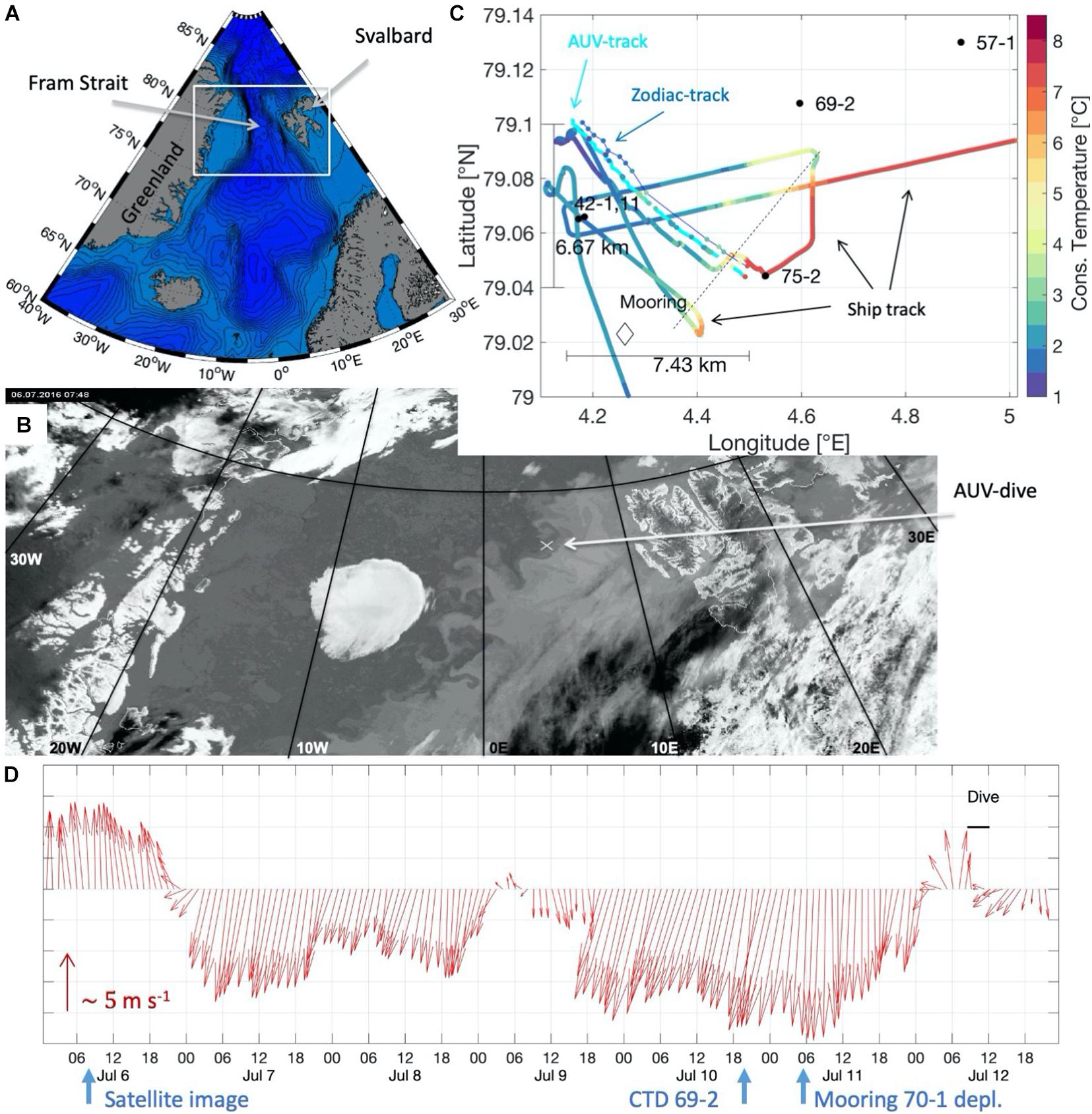
Figure 1. (A) Topographic map of the Nordic Seas and Fram Strait. The study region is marked with a white box. (B) Infrared image taken on 6 July, 7:48 UTC of Fram Strait (channel 3 data of the AVHRR/3 instrument on the NOAA 15 satellite). The approximate location of the AUV-dive is marked by the white cross. (C) Sea surface temperature measured by the ship’s thermosalinograph at 5 m depth, and by the AUV and zodiac at 1 m depth. The AUV-track is marked in cyan, the zodiac-track is marked in blue. Black dots give shipboard CTD-station locations with station numbers. The black diamond indicates the position of the mooring. (D) One hour-averaged wind direction (arrow pointing into the down-wind direction) and wind speed (relative arrow length). The timing of the satellite image, the CTD station 69-2 and the mooring deployment 70-1 are indicated below the plot. The black bar indicates the time of the dive.

The AUV dive pattern was designed to cross the front perpendicularly, undulating between the surface and 60 m depth on a zig-zag patch, collecting high-resolution profile data along a 10 km-long transect (Tippenhauer et al., 2018). The AUV was operated using a constant propeller rotation (rpm) resulting in a speed of approximately 1.5 m s^–1 with an average heading 333°T. The dive started at 79.04°N, 4.5°E within the 7–8°C warm AW, crossed the front in a north-westward direction, and ended at around 79.1°N, 4.15°E, on the cold side of the front (cyan line in Figure 1C). On a parallel transect, approximately 400 m north of the AUV track (blue line in Figure 1C), we operated a small, handheld CTD from a zodiac (SBE19plus, Tippenhauer et al., 2018). At the same time, the ship recorded the sea surface temperature (Soltwedel and Rohardt, 2017) along a parallel transect south of the AUV (Figure 1C). All oceanographic parameters were computed using the TEOS-10 GSW toolbox (McDougall and Barker, 2011). We exclusively use absolute salinity and conservative temperature in this study.

Atmospheric parameters are recorded continuously onboard Polarstern by a meteorological observation system (König-Langlo, 2016). Prevailing winds 5 days before the dive were north-easterly with variable strength, as shown in Figure 1D.

Instruments

Polarstern’s TSG system is a SEACAT SBE21 coupled with a Digital Oceanographic Thermometer SBE38 (Seabird Electronics). The water intake is located 5 m below the surface. Additionally, a FerryBox (-4H-JENA engineering GmbH) measures near-surface chlorophyll a concentrations. The ship’s CTD was equipped with the standard SBE911plus setup including double sensors for temperature and conductivity, with an additional SBE43 for oxygen and a WET Labs ECO-AFL/FL for fluorescence observations (Tippenhauer et al., 2017). The AUV is a 4.7 m long Bluefin 21 vehicle (Bluefin Robotics, operated by AWI) equipped with a SBE49 FastCAT CTD probe (Seabird Electronics). During this campaign, the AUV carried an upward looking Acoustic Doppler Current Profiler (ADCP) 300 kHz Workhorse Monitor (Teledyne RD Instruments) and a turbulence profiler (Rockland Scientific, MicroPod System) for velocity shear. Unfortunately, we could not derive turbulent dissipation rates due to broadband noise contamination. The algorithm for noise reduction developed for previous studies (Tippenhauer et al., 2015) for a different AUV-turbulence-profiler system could not be applied, due to the more broadband nature of the noise here. In the future an improved mounting might solve this issue. As the water depth in the study was deeper than the vehicle’s Doppler Velocity Log, the accuracy of the navigation data was reduced. During the dive we tracked the AUV path acoustically, such that the method described in Wulff and Wulff (2015), for correcting the navigation data, could be applied in post processing. This provides us with more accurate positions of the AUV, compared to positions estimated by dead reckoning only. For processing the ADCP data, we used a modified version of the SACDP processing toolbox originally by GEOMAR. The AUV is further equipped with an upward-looking sensor for photosynthetically active radiation (PAR, Irradiance, Satlantic, Canada), a nitrate sensor (Deep Ocean SUNA, Seabird), a dissolved oxygen sensor (electrochemical, fast responding profiling version, SBE43) and a fluorometer (C7 c, Turner Designs) to determine fluorescence of chlorophyll a, as a proxy for biomass. Water samples collected by the vehicle’s water sample collector (Wulff et al., 2010) were analyzed for nutrient concentrations (nitrate, nitrite, silicate, and phosphate). Sample-derived nitrate concentrations were used to calibrate the raw signal of the SUNA sensor. The raw fluorescence measurements of the C7 fluorometer were not calibrated with sample material of this specific dive, as the sample collector did not take samples within the chlorophyll maximum region, but in a region with rather homogenous chlorophyll concentrations. The derived calibration curve thus does not stretch over a sufficient range to be suitable for calibration purposes. For this reason, the chlorophyll a concentrations presented in this paper were calculated based on a calibration from a previous dive in 2013. Nonetheless, it should be pointed out that the fluorometer was saturated within the maximum fluorescence area, a phenomenon that we had not observed before using identical fluorometer settings.

Dive Pattern and Data Interpolation

The dive pattern was designed to include different phases to measure different parameters. The zig-zag pattern was chosen to record properties such as temperature, salinity, chlorophyll a, nitrate and oxygen in the water column in high-resolution. In-between the individual “Sawtooth’s” of the zig-zag pattern, segments along constant pressure were introduced to record the velocity structure above the AUV using the upward looking ADCP. For the PAR data, every second to third ascend of the AUV was performed as a so-called float-maneuver, where the propulsion of the AUV was turned off, resulting in a horizontal float to the surface, due to the residual buoyancy of the vehicle. This phase of the dive is necessary as the PAR sensor data is reliable only if the sensor is oriented perpendicular to the incoming light.

As this dive pattern results in a rather special data set with irregular spacing in all dimensions, careful evaluation and interpolation is necessary. After sensor calibration and correction of the position as described in Wulff and Wulff (2015), the data was manually checked and divided into different dive phase segments. Then, the hydrographic data from the down- and up-casts were first interpolated onto a regular pressure grid, and subsequently interpolated on a regular horizontal spacing. For all considerations that require hydrographic and velocity data, both were interpolated on the same grid in a third step. This is necessary as the velocity data are available only for those segments in-between down- and up-casts, as the AUV was able to record the velocity above it only during those dive-phases. This grid however, is not regular in the horizontal, since the dive pattern was not regular. The spacing varies between 256 and 1,055 m. Those gridded data were used to compute all derived quantities that will be introduced in the following section.

Conducting frontal studies with comparably slow vehicles as gliders or AUVs always includes the problem of a potential distortion from the planned path. In the study of Carpenter et al. (2020) an autonomous glider, planned to dive on an east-west oriented track was forced on a southward path due to strong currents. Also, for our study, it cannot be ruled out that the currents might have altered the planned dive track. However, our AUV was moving through the water with approximately 1.5 m s^–1, while we encountered maximum ocean currents of 0.3 m s^–1, and we therefore neglect the effect of a drifting feature in this study.

Analysis of Frontal Processes

To understand the frontal processes, we analyzed the stratification and the velocity field and derived quantities such as the Richardson number (Ri), which relates the strength of stratification to velocity shear. Direct observations of turbulent kinetic energy dissipation rates are not available for this study due to technical problems. We therefore assess potential mixing processes and instabilities around the front based on geostrophic velocities and vorticity-based instability criteria. The direct velocity observations were rotated into along-front and cross-front components and vertically averaged in 4 m bins. The along-front component is then compared to the geostrophic velocities derived from 4 m vertically-averaged properties, by integrating the geostrophic shear from the lowest layer (55 m depth), assuming zero velocity. The buoyancy-frequency N² (where N² = db/dz,withb = −gρ_θ/ρ₀) was vertically averaged over 4 m bins and, combined with the total shear Sh² = (du/dz)² + (dv/dz)², provides the Richardson Number Ri = N²/Sh².

Generally, shear instabilities can arise when the velocity shear exceeds the fluid stratification, with the necessary condition of a local Ri of less than 0.25. Other forms of instabilities can also develop under various conditions. Gravitational instabilities occur if the stratification is unstable (N² < 0), resulting in vertical convection. Inertial or centrifugal instability arise due to the instability of fluid parcels to horizontal perturbations, when the equilibrium between different forces in the initial state (geostrophic or cyclostrophic balance) becomes unstable. If a horizontal velocity perturbation is advected in meridional direction, it can be either reinforced or dampened by the Coriolis force, depending on the direction and amplitude of the perturbation. If the Coriolis force reinforces the perturbation, an inertial instability forms (Haine and Marshall, 1998); Smyth and Carpenter, 2019). Symmetric instabilities can form in a situation with stable stratification (N² > 0) and a two-dimensional flow (such as at a front), with a vertical (dv/dz) and cross-frontal velocity gradient (dv/dx). The cross-frontal velocity gradient can stabilize or destabilize the flow. If symmetric instability occurs, convection is no longer vertical as is the case for gravitational instability. Due to thermal wind shear in a stratified, rotating fluid, convection will be slantwise and lead to an exchange in the vertical and horizontal at the same time (Haine and Marshall, 1998). This slantwise convection will leave a stably stratified water column and restore the potential vorticity to zero.

Mathematically, these instabilities can be characterized based on potential vorticity. In a stably stratified flow, inertial and symmetric instabilities can develop if the Ertel Potential Vorticity PV (q) and the Coriolis parameter (f) have opposite signs (Thomas et al., 2013; Peng et al., 2020):

where $\widehat{\mathbf{\text{k}}}$ is the upward unit vector, u is the velocity vector, and b = −gρ_θ/ρ₀ again the buoyancy, with g – the acceleration due to gravity, ρ_θ – the potential density, and ρ₀ = 1026 kg m^–3 the reference density. By decomposing q into the vertical (q_ζ) and the baroclinic (q_bc) components it can be distinguished whether the conditions allow for symmetric or for inertial/centrifugal instabilities (Peng et al., 2020). The vertical (q_ζ) and the baroclinic (q_bc) components are defined following Peng et al. (2020):

where the term dv/dx describes the change of the along-front velocity component across the front while db/dx describe the change of the density field across the front. The term dv/dz describes the vertical shear of the along-front velocity component and N² = db/dz is again the square of the buoyancy frequency. Symmetric instability (SI) is expected if |fq_bc| > fq_ζ with fq_ζ > 0 (cyclonic absolute vorticity), while inertial/centrifugal instabilities are expected if fq_ζ < 0 (anticyclonic absolute vorticity). Inertial/centrifugal instabilities derive their energy from lateral shear, whereas symmetric instabilities grow at the expense of vertical shear.

Results

Water Masses at the Front

The roughly 10 km-long AUV transect across a strong front separating AW from PW was characterized by a complex water mass structure with wide ranges in temperature (−2 to 7°C), salinity (33–35), chlorophyll-a (0–10 μg L^–1), nitrate (0–10 μmol L^–1) and oxygen saturation (90–115%) (Figure 2). For easier orientation, we use the kilometer-scales at the top of Figure 2A to point out relevant features along the transect. The surface showed a complex water mass distribution and was dominated by two fronts. The first was located about 1 km into the transect (km-1, right blue arrow top of Figure 2), where the temperatures decreased sharply from 7 to 2°C. The second front was located near km-6 (left blue arrow top of Figure 2), with warmer (1°C) water extending from the surface down to about 20 m at km-8. Surface waters carried temperatures of about 1°C, underlain by near-freezing PW (red contour in Figure 2A). This cold layer was thickest near the interface between PW and the warm AW reaching down to 45 m between km-2 and km-4. Here, the temperature changed from below 1 to 7°C, over a distance of less than 1,000 m. On the warm side of the front (km-0 to 2), the water column was well mixed down to 45 m (Figure 2A). West of km-3, the water was colder, fresher and more stratified (Figure 2). However, this front was density-compensated, as there was also a strong salinity gradient (Figure 2B). Towards the western end of the transect (km-9), the cold and fresh layer thinned and was confined to depths between 25 and 35 m. The water below this cold layer was less stratified, warmer and more saline. Physical properties in temperature-salinity space (Figure 3) indicate that two water masses have just recently come into contact. The AW with densities of 27.1–27.6 kg m^–3 (potential density with reference to 0 dbar) being warmer than 3°C and the modified AW and surface PW with densities of 26.0–27.8 kg m^–3 and temperatures below 3°C (Figure 3). The densest waters of more than 27.6 kg m^–3 were found on either side of the front at about 50 m (marked by black and cyan boxes in Figures 2, 3). These two water masses are similar in temperature and salinity but spatially separated, indicating that they have not been in contact before, as they show no sign of mixing (Figure 3). The water masses with the two temperature extremes (AW of 8°C and near-freezing PW) throughout the section, had a density of less than 27.6 kg m^–3. The TS-diagram shows that mixing between these two water masses occurs at their interface (cabbeling, marked with two black arrows and a blue box in Figure 3), creating denser water of more than 27.6 kg m^–3. This water subducted and was found deeper in the water column (blue box Figures 2, 3).

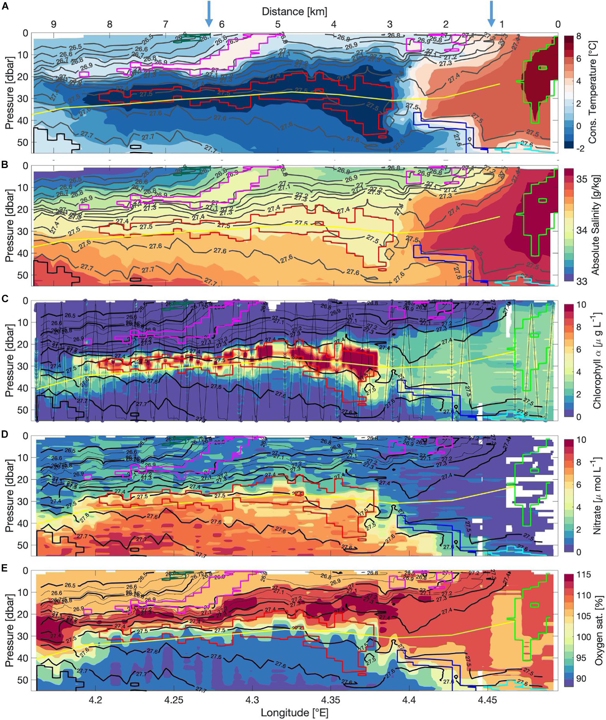
Figure 2. (A) Conservative temperature (°C), (B) absolute salinity (g/kg), (C) chlorophyll a (μg L^–1), (D) nitrate (μ mol L^–1) and (E) oxygen saturation (%). Black contour lines indicate potential density. Individual AUV-profiles are marked in black with a scatter plot showing the single-point measurements in panel (C). Yellow line indicates the euphotic depth. Blue arrows at the top of panel (A) indicate the position of the two fronts. Colored contour line-boxes indicate different water masses [green – Atlantic Water, red – Polar Water, yellow, green and magenta – different types of surface waters, black and cyan – different types of colder and slightly fresher Atlantic Water, blue – mixed water originating from cabbeling (compare Temperature-salinity-diagram in Figure 3)].

Figure 3. Temperature-salinity-properties along the AUV-transect. Colors indicate the pressure (dbar) of the individual measurements. Black contour lines indicate potential density (reference 0 dbar). Colored boxes indicate different water masses (green – Atlantic Water, red – Polar Water, yellow, green and magenta – different types of surface waters, black and cyan – different types of colder and slightly fresher Atlantic Water, blue – mixed water originating from cabbeling. Mixing occurred along the 27.6 isopycnal indicated by the two black arrows. Same colored-boxes are used to indicate the location of these water masses along the section in Figures 2, 4. The thick black line indicates the freezing point temperature.

Biogeochemistry of the Front

A patch of extraordinary high chlorophyll a concentrations exceeding 10 μg L^–1 (Figure 2C) dominated the chlorophyll distribution along the AUV-transect. The patch was observed inside the cold, stratified water lens with nitrate concentrations of 2–6 μmol L^–1 (Figure 2D). Above this patch in the upper 25 m, the nitrate concentration was less than 2 μmol L^–1. Below 25 m, concentrations increased to 6–9 μmol L^–1 underneath the chlorophyll a patch just below the euphotic depth (yellow contour in Figure 2) where the stratification was weaker. The euphotic depth is defined as the level where the light decreases to 1% of the light available at the surface. The euphotic depth derived from the AUV-based PAR sensor occupied the 30–40 m depth range (Figure 2). At the eastern edge of the section (km-0 to 2), chlorophyll a concentrations of 2–4 μg L^–1 were found down to 55 m depth, thus, to at least 20 m below the euphotic depth. The nitrate concentration there was close to 0 μmol L^–1 (Figure 2D). The oxygen saturation field contrasted that of nitrate, with the lowest concentrations found within the high-nitrate dome, indicative of higher water mass age. Just above the chlorophyll maximum as well as on the warm side of the front (km-1), the water was supersaturated with oxygen (Figure 2E). The supersaturation just above the chlorophyll maximum and below the pycnocline indicates active photosynthesis and the shielding effect of the pycnocline preventing outgassing (Anderson, 1969; Shulenberger and Reid, 1981), consistent with previous long-term Glider observations off the Washington coast (Perry et al., 2008). The remarkable feature among the distribution of biogeochemical properties along the transect is thus the 5–10 m-thick band of high chlorophyll, located immediately above the euphotic depth. The upper part of the elevated dome of nitrate ends abruptly at the euphotic depth which indicates nitrate supply and utilization, further underlined by supersaturated oxygen levels.

Dynamics of the Front

The warmer eastern side of the front (km-0 to 2) was characterized by weak stratification, with buoyancy-frequencies (N²) close to zero almost throughout the water column (Figure 4A). When resolved in 1 m bins (not shown), gravitationally unstable stratification with negative N² was found at the interface of the PW and AW water masses, indicating the effect of cabbeling (blue box Figure 3 and magenta color at km-3 in Figure 4A). Further, gravitationally unstable regions in the 1 m binned data were found near km-8.5 at 33 m, around km-9 at 26 m, and around km-6, between 5 and 20 m water depth (not visible in the Figure 4A as this figure shows 4 m resolution). Comparably strong stratification was observed in a band above the cold water patch, deepening from 10 m at km-2 to 20 m at km-7/8. A second and weaker band was found at 10 m in between km-7 and km-8.

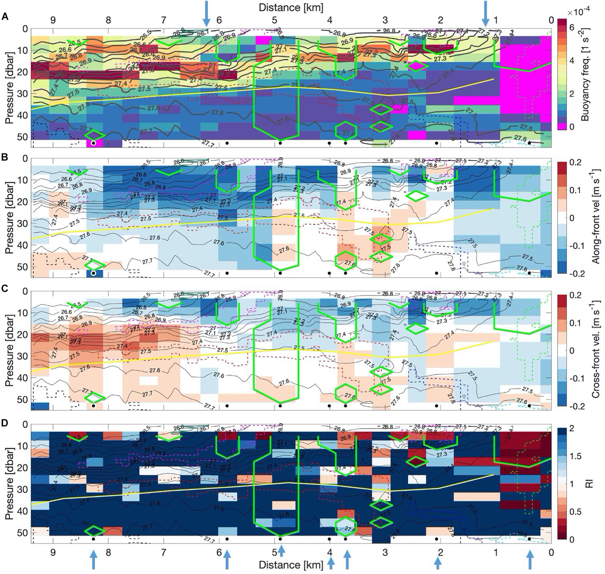
Figure 4. (A) Buoyancy-frequency N² (s^–2) from upward and downward profiles of the AUV computed over 4 m bins, (B) Along-front velocity component (ms^–1) computed over 4 m bins. Blue colors indicate south-westward velocities (out of the page). Red colors indicate north-eastward velocities (into the page). (C) Cross-front velocity component (ms^–1) computed over 4 m bins. Red colors indicate north-westward velocities (towards the left of the plot). Blue colors indicate south-eastward velocities (towards the right of the plot). (D) Richardson Numbers (colored circles) computed over 4 m bins. All: Black contour lines indicate potential density. Yellow line indicates the euphotic depth. Colored, dashed contour line-boxes indicate different water masses (compare Figures 2, 3). The thick green contour line indicating areas with negative Ertel potential vorticity. Blue arrows at the top indicate the position of the two fronts. The black dots at 53 m and the blue arrows mark the locations of the single profiles shown in Figure 5.

The along-front velocity component indicates that the surface layer moved almost homogeneously in down-front direction (i.e., south-westward, out of the page, blue colors in Figure 4B). The strongest down-front flow with more than 0.2 m s^–1 was observed above the band of high stratification indicative of a frontal jet. Below the frontal jet as well as within the AW region, weaker south-westward flow of around 0.1 m s^–1 was observed (blue colors in Figure 4B). Up-front velocities were only observed between km-2 and km-6 mostly below 20 m and at the western edge of the section at 20 m and at 45 m water depth. Cross-frontal velocities in the surface layer were generally weak (mostly below 0.1 m s^–1) and oriented south-eastward, leading to flattening of density contours and hence to weakening of the surface fronts (blue colors in Figure 4C). Below this, even weaker velocities of less than 0.05 m s^–1 were observed. Only at the western side of the front between 15 and 30 m, comparably strong velocities occurred towards the north-west reaching 0.15 m s^–1 (i.e., down-gradient flow). Within or slightly below this down-gradient flow, the stratification was weak or close to being gravitationally unstable (Figure 4A).

To gain insight into possible mixing events, we screened the data for the sensitivity to the various forms of instabilities described in the data and methods-section. We present a subset of the data in Figure 5. In particular we contrast the geostrophic flow derived from thermal wind with the observed velocity (top of Figure 5, panels 1–7), relate the shear with stratification (panels 8–14), and present the vertical, baroclinic, and total potential vorticity (panels 15–21). First, we assess whether the flow is in geostrophic balance or whether it is ageostrophic. In geostrophic balance the flow exhibits a balance between the Coriolis force and the pressure gradient force. In absence of this balance, the flow becomes ageostrophic, wherein other forces also become important, such as friction. The along-front velocities were mostly not in geostrophic balance (top of Figure 5 panels 1–7). On the warm side of the front, the flow was close to geostrophic balance at the surface, but not below 10 m, where the difference between geostrophic and measured velocities increased with depth (Figure 5 panel 7). Further to the west, observed and geostrophic velocities differed in direction but were both weak. At km-4 the observed velocities were comparably strong and not geostrophically balanced (Figure 5 panel 4), while the flow was closest to geostrophic balance throughout all of the transect at km-4.9, with a frontal jet above 20 m (Figure 5 panel 3). The down-front velocities extended to km-8 and 30 m depth although geostrophic velocities indicated weaker down-front or even up-front velocities (Figure 5 panels 3-1). Concluding this section we note, that the flow is mostly not geostrophically balanced, which implies that other forces such as wind must have played a role in creating the observed patterns.

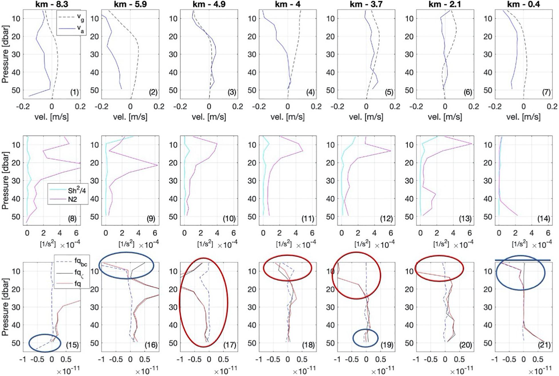
Figure 5. Selected profiles of the (1–7) geostrophic v_g and observed along-front velocity v_a, (8–14) stratification N² and total Sh²/4, for easier comparison with the critical Richardson number (Ri = 1/4 or, equivalently, N² = Sh²/4). (15–21) The vertical (fq_ζ), baroclinic (fq_bc), and total potential vorticity (fq)component. The locations of the single profiles used here, are marked in Figure 4 with a black dot at 53 m and a blue arrow.

To assess the likelihood for shear instabilities we relate the shear with stratification (middle of Figure 5, panels 8–14). Whenever the Sh²/4 curve exceeds the N² curve, shear instabilities may potentially occur. This is the case only on the warm side of the front between 20 m and 40 m depth (Figure 5 panel 14) as well as at km-5.9 at the surface (Figure 5 panel 9). In areas where N² is negative, gravitational instabilities will form and lead to convective mixing, such as on the warm side of the front between 20 m and 40 m depth (Figure 5 panel 14). Hence, gravitational instabilities are present on the warm side of the front at km-0.4 (Figure 5 panel 14) and shear instabilities might occur at km-5.9 at the surface (Figure 5 panel 9). Thus, shear instabilities might occur, but play only a minor role. Instead, other types of instabilities might be more relevant, which we assess in the following.

The different components of the vorticity provide a measure for the rotative forces within the flow, which arise due to gradients in the density and velocity field. Different forms of instabilities can occur if the Ertel potential vorticity is negative, as described in the methods-section. Areas with negative Ertel potential vorticity are indicated with a green contour in Figures 4A–D. In Figure 5 (panels 15–21), circles mark those locations where symmetric (blue) and inertial/centrifugal (red) instabilities are possible. Symmetric instabilities are indicated on the warm side of the front at km-0.4 and at km-5.9 above 20 m (Figure 5 panel 21 and 16). Furthermore, below 40 m at km-3.1 (not shown in Figure 5), at km-3.7 and at km-8.3 (Figure 5 panel 19 and 15). Vorticities close to zero might be a sign of past symmetric instabilities, which might be the case at km-4, km-5.9 (Figure 5 panel 18 and 16), and km-7.5 (not shown in Figure 5). Indications for inertial/centrifugal instabilities in the upper 20 m were found at km-2.1, km-3.7, and km-4 (Figure 5 panel 18–20), while they were found throughout the upper 50 m at km-4.9 (Figure 5 panel 17). At most of the other locations the layer below 20 m was characterized by Ertel potential vorticities of just above zero, and thus not directly indicative of an instability.

Overall, we found numerous indications for symmetric and inertial/centrifugal instabilities at several locations along the front. Gravitational and shear instabilities were present, but play a minor role. The different types of instabilities discussed here are illustrated in Figure 6. Apart from exceeding the instability thresholds described above, the vorticity was regularly near-zero between km-5 and km-8 below 30 m. This could be a sign of previous symmetric instabilities that would set the vorticity to zero but would not break down the stratification, due to the slantwise circulation of symmetric instabilities (Haine and Marshall, 1998). Such a slantwise circulation would result in vertical mixing and thus induce vertical fluxes from the high-nutrient reservoir below the pycnocline into the sunlit layer above. This could therefore provide a key contribution to fuel the substantial chlorophyll patch as well as to potentially sustain active growth throughout the summer.

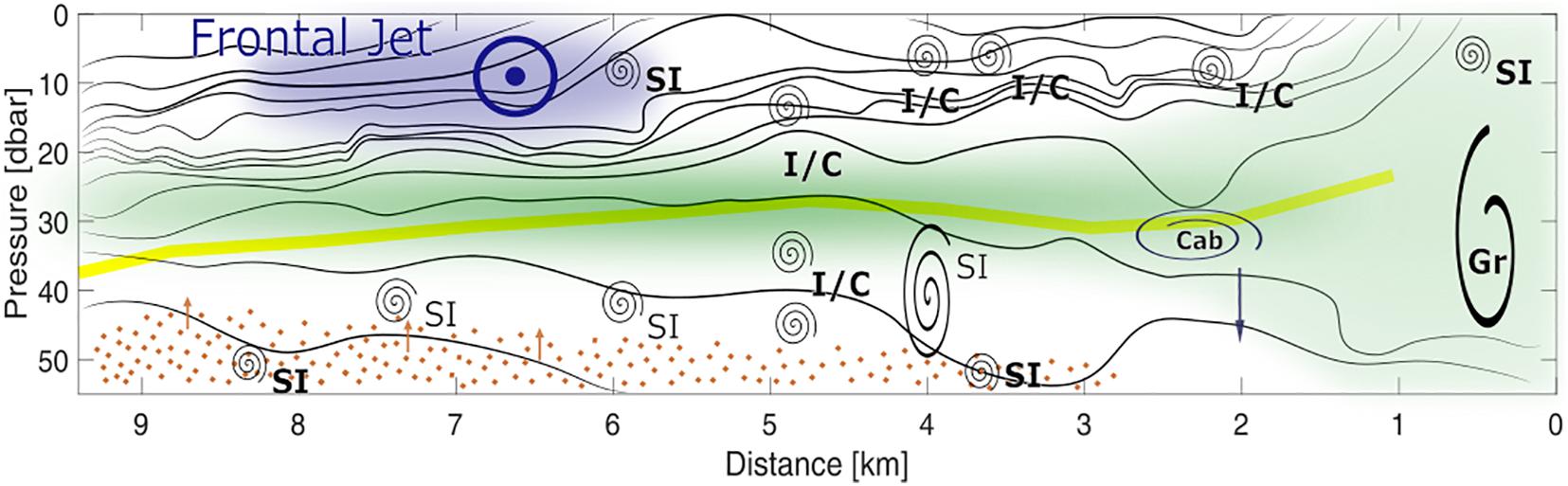
Figure 6. Schematic illustrations of the major observed features and processes. Black lines – density contours, green patch – phytoplankton patch, yellow line – euphoric depth, blue patch – frontal jet coming out of the page, brown dots and arrows – nitrate and nitrate flux. The spirals indicate mixing in general while distinct mixing processes are indicated by text with Gr – gravitational instability, cab – cabbeling with the arrow indicating densification and sinking, I/C – inertial/centrifugal instabilities, and SI – symmetric instabilities. Bold text indicates where the required conditions were met while normal font indicates locations where the vorticity was close to zero which might be a sign of previously past symmetric instabilities.

Discussion

The AUV-observations revealed a complex physical and biogeochemical water column structure on small scales and highlight the role of vertical nitrate fluxes to sustain sub-surface phytoplankton blooms. Apparently, the spring bloom had already depleted the surface water nitrate by the time of our survey in early July 2016, and was shielded from the deeper nitrate reservoir by strong stratification. With the euphotic zone reaching only down to 30 m, the small-scale processes reported here thus seem to provide a mechanism needed to support phytoplankton growth later in the season.

Subsurface chlorophyll maxima (SCM) are observed throughout the Arctic Ocean (Brown et al., 2015). Besides SCM depths of 60 m in the Canada Basin, depths around 30 m have been reported for most Arctic shelf regions, such as on the Chukchi Sea shelf (Brown et al., 2015) or the Kara Sea (Demidov et al., 2018). Once the spring bloom depletes the upper ocean nutrients, the chlorophyll maximum deepens until it reaches a depth range that allows sustained production, dependent on the nutricline and light availability (i.e., euphotic depth). Conditions may be less favorable in regions receiving enhanced input of suspended particles and dissolved substances such as CDOM from large rivers, where most of the PAR is absorbed in the upper few meters of the water column (Soppa et al., 2019). Changing Arctic conditions associated with changes in stratification and the upper ocean freshwater reservoir have led to increases in the observed (McLaughlin and Carmack, 2010) and projected (Steiner et al., 2016) depth of the nutricline, and thus the depth of SCM. Our AUV observed the SCM at around 30 m within the patch of cold PW, which agrees with the base of the euphotic depth, as measured by the AUV’s PAR sensor. The low-chlorophyll western edge of the transect indicates a deeper euphotic layer down to 40 m as opposed to the 30 m in the high-chlorophyll patch, which may be due to a self-shading effect of the SCM.

Strong north-easterly winds of more than 10 m s^–1 prevailing for 2.5 days before the experiment, may have intensified the front (via Ekman transport and frontogenesis), which was aligned at 63°T. These sustained winds may have caused an increase in baroclinicity and developed an ageostrophic frontal jet, which provided an environment susceptible for instabilities and mixing to flux nitrate into the euphotic layer. At the time of our survey, it is likely that the front had already started to relax (i.e., to flatten density contours) as winds decreased and shifted to south-easterly.

Conditions underneath some parts of the observed phytoplankton patch were favorable for different forms of instabilities, which supports the assumption that nitrate may be injected into the euphotic layer to sustain the plankton patch. Instabilities might have occurred there earlier, when the wind was stronger or might still occur intermittently. The weak stratification of the water column also indicates that mixing was either intermittent or not strong enough to entirely remove the stratification. In the case of symmetric instabilities, slantwise convection would flux nutrients upwards without eroding vertical stratification. West of km-3 mixing did not completely destabilize the water column and mix down phytoplankton cells, as observed on the eastern side of the front (Figure 2C). However, the lower rim of the phytoplankton patch is less sharp compared with the upper rim, indicating that some phytoplankton cells may have been mixed into deeper waters (Figure 2C). Intermittent nitrate injections into the sunlit layer might thus explain the extraordinarily high chlorophyll a values as derived from the AUV’s fluorometer.

The growth and subsequent temporal evolution of this high chlorophyll patch remains unknown, but likely partially depended on the physical evolution of the front. Water samples from this high chlorophyll a layer were not collected, and therefore, we have no information about plankton diversity, primary production rates, nutrient composition, or carbon uptake. However, based on the water mass assessment (Figure 3), we can assume that the planktonic species at the cold and warm sides of the front are distinct from each other, as these water masses had not previously mixed. Such a distinction of plankton communities was shown at a filament in Fram Strait based on an extensive water sampling program as part of a multi-disciplinary study (Fadeev et al., 2021).

In order to gain insights regarding spatial and temporal extent of the front and the phytoplankton patch, we investigate complementary datasets comprised of a parallel zodiac transect and nearby ship-based CTD profiles and mooring deployments. Although at a lower resolution, the zodiac section reflected those features shown by the AUV transect, indicating that the front extended over a distance of at least 400 m (not shown). One ship-based CTD-profile collected 7.5 km north-east of the AUV-track (Figure 1) 1 day before the AUV-dive, showed an SCM of more than 15 μg L^–1 between 14 and 18 m depth (Figure 7B. Station PS99/069-2 at 79.1°N, 4.6°E collected on 10 July 2016). This SCM was located at the top of a cold water mass with temperatures of −1.55°C extending down to about 40 m (Figure 7A). This profile showed the same properties as observed in our AUV-section on the cold side of the front (Figure 2A, west of km-3). These complementary observations hence imply that the front extended far beyond the zodiac section and at least 7.5 km up-front, with a cold layer 5 m shallower and a chlorophyll maximum confined to a narrower band than compared to the AUV section. The chlorophyll measured from water samples (Nöthig et al., 2018) collected with the shipboard CTD from 17 m, however, only showed concentrations of 4.76 μg L^–1 (Figure 7B, filled circles). As a standard procedure, sensor-based CTD profiles are processed from the downcast only, while actual water samples are collected during the upcast. The time passed between up- and downcast depends on the water depth and might be substantial. We therefore compare the laboratory-measured chlorophyll a value with the downcast-profile, as well as with the point-measurement, when the CTD sampling bottles were closed during the upcast (Figure 7B empty circles). For instance, at station 69-2 the average value for all bottles closed at 17 m depth is 4.78 μg L^–1 and thus in very good agreement with the laboratory value of 4.76 μg L^–1, although strikingly different from the downcast value of 15 μg L^–1. This discrepancy can thus result from missing the thin chlorophyll patch or from lateral displacement of this small-scale feature relative to the ship. The samples taken within the SCM at station 42-11 and 57-1 also missed the maximum chlorophyll concentration (Figure 7B), which underlines the difficulties in accurately capturing the biomass in regions characterized by strong mesoscale activity.

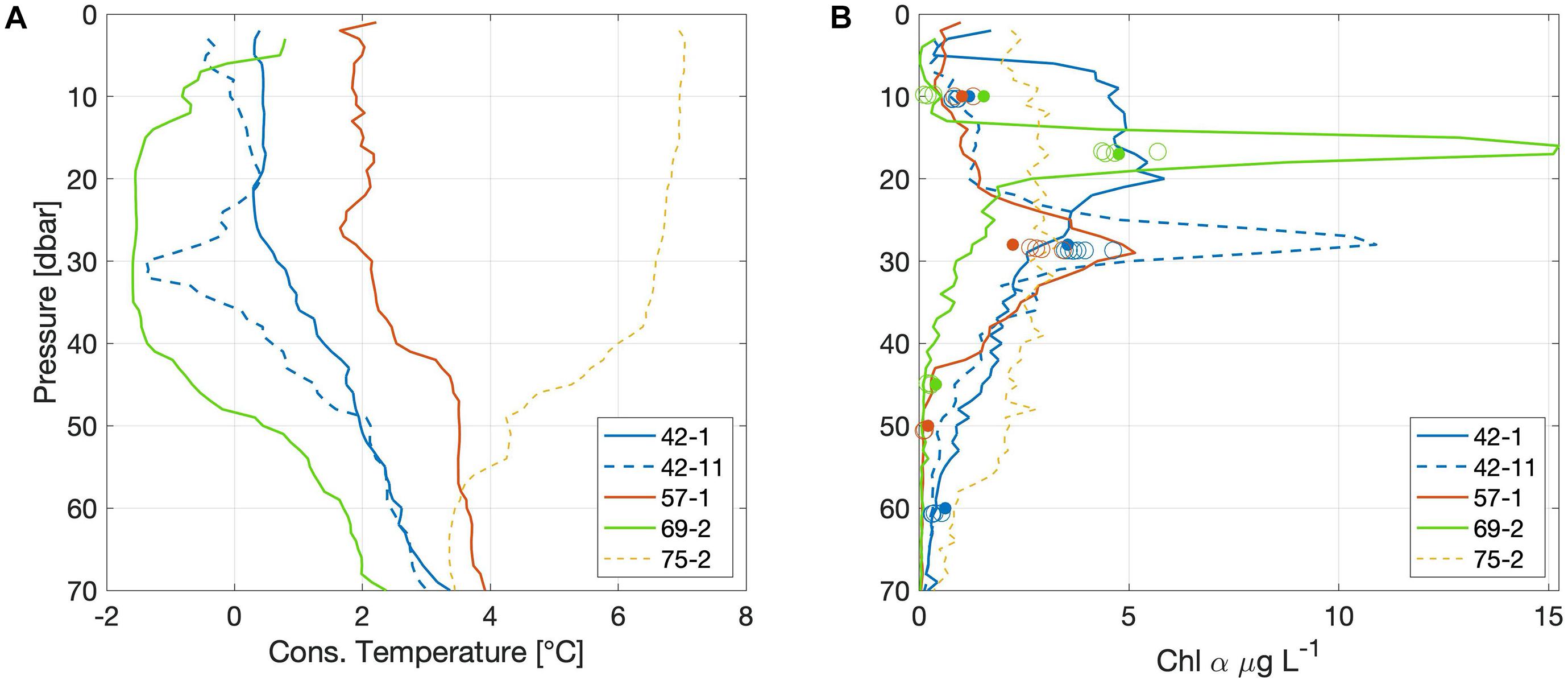
Figure 7. Profiles of (A) conservative temperature (°C), and (B) chlorophyll a (μg L^–1) from CTD-stations close to the AUV-dive location. Chlorophyll a concentration observed with the CTD sensor during the down- (continuous and dashed lines) and upcasts (empty circles, showing values associated with bottle data from selected depths), as well as concentrations measured from water samples (filled circles). Legends indicate station numbers and are shown in the map in Figure 1.

Additional spatial and temporal context of the front and the chlorophyll patch can be gained from a mooring deployed 5 km south of the AUV section (HG-IVS, PS99/0070-1 deployed at 79.023°N, 4.26°E on 11 July 2016, Figure 1C). This location also showed the presence of cold waters of −1.56°C at about 40 m, which remained present until 1.5 days after the dive. Thus, we assume the front extended another 5 km into the down-front direction. Finally, a mooring-based fluorometer installed at 28 m recorded (saturated) chlorophyll a values of more than 30 μg L^–1. In summary, three different fluorometers (two of them recorded saturated values) measured a subsurface phytoplankton patch with high chlorophyll a concentrations, extending over at least 14 km and over a period of at least 2 days. Observations such as these would be missed by satellites and traditional ship surveys. For example, Nöthig et al. (2020) analyzed a 25 year-long record of biological observations in Fram Strait, and found that the data are mainly driven by seasonal and spatial variability, rather than following a clear temporal trend. Here, we reiterate the importance of mesoscale processes, which are especially pronounced near fronts, meanders, or eddies as often found near the MIZ. Already in the 1980s, Niebauer and Alexander (1985) reported on observations of subsurface high chlorophyll patches due to interleaving water masses at the Bering Sea ice edge. Considering the increasing role of MIZ processes in a changing Arctic Ocean, and the importance of the Arctic ecosystem for carbon export, our findings underline the necessity for more coordinated 4-dimensional experiments, to better understand the physical and biogeochemical processes that are known to occur on scales too small to be captured in traditional surveys.

Summary and Conclusion

This paper presents results from a 10 km-long high-resolution AUV transect across a front separating warm AW from cold PW in Fram Strait as part of a coordinated frontal experiment carried out during an RV-Polarstern campaign in 2016. The AUV carried a CTD and biogeochemical sensors that captured a patch of substantial chlorophyll biomass centered around a depth of 30 m within a tongue of cold PW. The patch was located below the depth of maximum stratification, at the interface between high-nutrient water below, and nutrient-depleted water above this layer. The euphotic depth (i.e., 1%-PAR level) as determined with the AUV, was located within the phytoplankton patch around 30 m. These observations provide an example of an Arctic subsurface chlorophyll-maximum, featuring substantial chlorophyll concentrations in a thin (5–10 m) and narrow (5 km) band, that is easily missed by satellites or traditional ship-board surveys. The data gathered supports the hypothesis that the patch was fueled by nitrate fluxes into the euphotic layer, which can potentially sustain high productivity throughout the summer. Our observations indicate the importance of small-scale bio-physical processes in driving primary production near fronts. Frontal processes such as found in Fram Strait or near the MIZ are becoming increasingly important in a changing Arctic Ocean, and thus will require enhanced measurement efforts to observe and understand these features. In particular, vertical mixing processes are difficult to observe but are crucial to understand the increasing impact of vertical heat fluxes on the seasonal sea ice retreat, as well as to understand how nutrient fluxes may contribute to enhanced primary production in the future Arctic Ocean ecosystem.

Data Availability Statement

The data used throughout this study is available at https://doi.org/10.1594/PANGAEA.863804, https://doi.org/10.1594/PANGAEA.887855, https://doi.org/10.1594/PANGAEA.873153, https://doi.org/10.1594/PANGAEA.871949, and https://doi.org/10.1594/PANGAEA.896071.

Author Contributions

ST and TW designed and implement the study, performed the laboratory, and data analyses. ST drafted the manuscript with contributions from all authors. All authors contributed to the article and approved the submitted version.

Funding

This study is part of the project Frontiers of Arctic Marine Monitoring (FRAM) funded by the Bundesministerium für Bildung und Forschung (BMBF) and the project PEANUTS (grant number 03F0804A), co-sponsored by BMBF and the Natural Environment Research Council (NERC) within the Changing Arctic Ocean (CAO) program.

Conflict of Interest

The authors declare that the research was conducted in the absence of any commercial or financial relationships that could be construed as a potential conflict of interest.

Publisher’s Note

All claims expressed in this article are solely those of the authors and do not necessarily represent those of their affiliated organizations, or those of the publisher, the editors and the reviewers. Any product that may be evaluated in this article, or claim that may be made by its manufacturer, is not guaranteed or endorsed by the publisher.

Acknowledgments

We thank the members of the AUV team from AWI for their engagement during all phases of planning, preparing, testing, and improving, during as well as after the cruise. We thank Gerd Rohardt and Andreas Wisotzki for CTD data processing. We thank Janine Ludszuweit, Jonas Hagemann, Tim Küber and Florian Krauß for spending hours in the cold on the zodiac taking hand-CTD profiles. We thank Eva-Maria Nöthig, Torsten Kanzow, and Ralph Timmermann for helpful discussions. We also thank one reviewer and JC for improving this study through very helpful and constructive feedback.

References

Anderson, G. C. (1969). Subsurface chlorophyll maximum in the northeast pacific ocean. Limnol. Oceanogr. 14, 386–391. doi: 10.4319/lo.1969.14.3.0386
Arrigo, K. R., and van Dijken, G. L. (2015). Continued increases in arctic ocean primary production. Progr. Oceanogr. 136, 60–70. doi: 10.1016/j.pocean.2015.05.002
Beszczynska-Möller, A., Fahrbach, E., Schauer, U., and Hansen, E. (2012). Variability in atlantic water temperature and transport at the entrance to the arctic ocean, 1997–2010. ICES J. Mari. Sci. 69, 852–863. doi: 10.1093/icesjms/fss056
Brown, Z. W., Lowry, K. E., Palmer, M. A., van Dijken, G. L., Mills, M. M., Pickart, R. S., et al. (2015). Characterizing the subsurface chlorophyll a maximum in the chukchi sea and canada basin. Deep Sea Res. Part II Top. Stud. Oceanogr. 118, 88–104. doi: 10.1016/j.dsr2.2015.02.010
Carpenter, J. R., Rodrigues, A., Schultze, L. K. P., Merckelbach, L. M., Suzuki, N., Baschek, B., et al. (2020). Shear instability and turbulence within a submesoscale front following a storm. Geophys. Res. Lett. 47:e2020GL090365. doi: 10.1029/2020GL090365
Cherkasheva, A., Bracher, A., Melsheimer, C., Köberle, C., Gerdes, R., Nöthig, E. M., et al. (2014). Influence of the physical environment on polar phytoplankton blooms: a case study in the Fram Strait. J. Mari. Syst. 132, 196–207. doi: 10.1016/j.jmarsys.2013.11.008
Demidov, A. B., Gagarin, V. I., Vorobieva, O. V., Makkaveev, P. N., Artemiev, V. A., Khrapko, A. N., et al. (2018). Spatial and vertical variability of primary production in the Kara Sea in July and August 2016: the influence of the river plume and subsurface chlorophyll maxima. Polar Biol. 41, 563–578. doi: 10.1007/s00300-017-2217-x
Engelsen, O., Hegseth, E. N., Hop, H., Hansen, E., and Falk-Petersen, S. (2002). Spatial variability of chlorophyll-a in the marginal ice zone of the barents sea, with relations to sea ice and oceanographic conditions. J. Mari. Syst. 35, 79–97. doi: 10.1016/s0924-7963(02)00077-5
Fadeev, E., Wietz, M., von Appen, W.-J., Iversen, M. H., Nöthig, E.-M., Engel, A., et al. (2021). Submesoscale physicochemical dynamics directly shape bacterioplankton community structure in space and time. Limnol. Oceanogr. 66, 2901–2913. doi: 10.1002/lno.11799
Hattermann, T., Isachsen, P. E., von Appen, W. J., Albretsen, J., and Sundfjord, A. (2016). Eddy-driven recirculation of Atlantic water in Fram Strait. Geophys. Res. Lett. 43, 3406–3414. doi: 10.1002/2016gl068323
Haine, T., and Marshall, J. (1998). Gravitational, symmetric, and baroclinic instability of the ocean mixed layer. J. Phys. Oceanogr. 28, 634–658. doi: 10.1175/1520-0485(1998)028<0634:gsabio>2.0.co;2
König-Langlo, G. (2016). Meteorological Observations During POLARSTERN Cruise PS99.2 (ARK-XXX/1.2). Alfred Wegener Institute, Helmholtz Centre for Polar and Marine Research. Bremerhaven: PANGAEA, doi: 10.1594/PANGAEA.863804
Lewis, K. M., van Dijken, G. L., and Arrigo, K. R. (2020). Changes in phytoplankton concentration now drive increased arctic ocean primary production. Science 369, 198–202. doi: 10.1126/science.aay8380
McDougall, T. J., and Barker, P. M. (2011). Getting Started With TEOS-10 and the Gibbs Seawater (GSW) Oceanographic Toolbox. SCOR/IAPSO WG127, 28.
McLaughlin, F. A., and Carmack, E. C. (2010). Deepening of the nutricline and chlorophyll maximum in the Canada Basin interior, 2003–2009. Geophys. Res. Lett. 37:L24602.
Niebauer, H. J., and Alexander, V. (1985). Oceanographic frontal structure and biological production at an ice edge. Contin. Shelf Res. 4, 367–388. doi: 10.1016/0278-4343(85)90001-9
Nöthig, E. M., Ramondenc, S., Haas, A., Hehemann, L., Walter, A., Bracher, A., et al. (2020). Summertime chlorophyll a and particulate organic carbon standing stocks in surface waters of the fram Strait and the Arctic Ocean (1991–2015). Front. Mari. Sci. 7:350. doi: 10.3389/fmars.2020.00350
Nöthig, E. M., Nadine, K., and Christiane, L. (2018). Chlorophyll a Measured on Water Bottle Samples During POLARSTERN Cruise PS99.2 (ARK-XXX/1.2). Alfred Wegener Institute, Helmholtz Centre for Polar and Marine Research. Bremerhaven: PANGAEA, doi: 10.1594/PANGAEA.887855
Randelhoff, A., Holding, J., Janout, M., Sejr, M. K., Babin, M., Tremblay, J. É, et al. (2020). Pan-arctic ocean primary production constrained by turbulent nitrate fluxes. Front. Mari. Sci. 7:150.
Peng, J. -P., Holtermann, P., and Umlauf, L. (2020). Frontal instability and energy dissipation in a sub-mesoscale upwelling filament. J. Phys. Oceanogr. 50, 2017–2035. doi: 10.1175/JPO-D-19-0270.1
Perrette, M., Yool, A., Quartly, G. D., and Popova, E. E. (2011). Near-ubiquity of ice-edge blooms in the Arctic. Biogeosciences 8:515. doi: 10.5194/bg-8-515-2011
Perry, M. J., Sackmann, B. S., Eriksen, C. C., and Lee, C. M. (2008). Seaglider observations of blooms and subsurface chlorophyll maxima off the Washington coast. Limnol. Oceanogr. 53, 2169–2179. doi: 10.4319/lo.2008.53.5_part_2.2169
Schourup-Kristensen, V., Wekerle, C., Danilov, S., and Völker, C. (2021). Seasonality of mesoscale phytoplankton control in eastern fram strait. J. Geophys. Res. Oceans 126:e2021JC017279. doi: 10.1029/2021JC017279
Serreze, M. C., Holland, M. M., and Stroeve, J. (2007). Perspectives on the arctic’s shrinking sea-ice cover. Science 315, 1533–1536. doi: 10.1126/science.1139426
Shulenberger, E., and Reid, J. L. (1981). The Pacific shallow oxygen maximum, deep chlorophyll maximum, and primary productivity, reconsidered. Deep Sea Res. Part A Oceanogr. Res. Papers 28, 901–919. doi: 10.1016/0198-0149(81)90009-1
Slagstad, D., Wassmann, P. F., and Ellingsen, I. (2015). Physical constrains and productivity in the future Arctic Ocean. Front. Mari. Sci. 2:85.
Smith, S. L., Smith, W. O., Codispoti, L. A., and Wilson, D. L. (1985). Biological observations in the marginal ice zone of the East Greenland Sea. J. Mari. Res. 43, 693–717. doi: 10.1357/002224085788440303
Smyth, W., and Carpenter, J. (2019). Instability in Geophysical Flows. Cambridge: Cambridge University Press, doi: 10.1017/9781108640084
Soltwedel, T., and Rohardt, G. (2017). Continuous Thermosalinograph Oceanography Along POLARSTERN Cruise Track PS99.2 (ARK-XXX/1.2). Alfred Wegener Institute, Helmholtz Centre for Polar and Marine Research. Bremerhaven: PANGAEA, doi: 10.1594/PANGAEA.873153
Soppa, M. A., Pefanis, V., Hellmann, S., Losa, S. N., Hölemann, J., Martynov, F., et al. (2019). Assessing the influence of water constituents on the radiative heating of laptev sea shelf waters. Front. Mar. Sci. 6:221. doi: 10.3389/fmars.2019.00221
Steiner, N. S., Sou, T., Deal, C., Jackson, J. M., Jin, M., Popova, E., et al. (2016). The future of the subsurface chlorophyll-a maximum in the Canada Basina model intercomparison. J. Geophys. Res. Oceans 121, 387–409. doi: 10.1002/2015JC011232
Stroeve, J., Holland, M. M., Meier, W., Scambos, T., and Serreze, M. (2007). Arctic sea ice decline: faster than forecast. Geophys. Res. Lett. 34:L09501. doi: 10.1029/2007GL029703
Strong, C., and Rigor, I. G. (2013). Arctic marginal ice zone trending wider in summer and narrower in winter. Geophys. Res. Lett. 40, 4864–4868. doi: 10.1002/grl.50928
Taylor, R. L., Semeniuk, D. M., Payne, C. D., Zhou, J., Tremblay, J. É, Cullen, J. T., et al. (2013). Colimitation by light, nitrate, and iron in the Beaufort Sea in late summer. J. Geophys. Res. Oceans 118, 3260–3277. doi: 10.1002/jgrc.20244
Thomas, L. N., Taylor, J. R., Ferrari, R., and Joyce, T. M. (2013). Symmetric instability in the gulf stream. Deep Sea Res. 91, 96–110. doi: 10.1016/j.dsr2.2013.02.025
Tippenhauer, S., Dengler, M., Fischer, T., and Kanzow, T. (2015). Turbulence and finestructure in a deep ocean channel with sill overflow on the mid-Atlantic ridge. Deep Sea Res. Part I Oceanogr. Res. Papers 99, 10–22. doi: 10.1016/j.dsr.2015.01.001
Tippenhauer, S., Torres-Valdés, S., Fong, A. A., Krauß, F., Huchler, M., and Wisotzki, A. (2017). Physical Oceanography During POLARSTERN Cruise PS99.2 (ARK-XXX/1.2). Alfred Wegener Institute, Helmholtz Centre for Polar and Marine Research. Bremerhaven: PANGAEA, doi: 10.1594/PANGAEA.871949
Tippenhauer, S., Wulff, T., Lehmenhecker, S., and Hagemann, J. (2018). Autonomous Underwater Vehicle PAUL Observations During POLARSTERN Cruise PS99.2. Bremerhaven: PANGAEA, doi: 10.1594/PANGAEA.896071
Tremblay, J. É, and Gagnon, J. (2009). The Effects of Irradiance and Nutrient Supply on the Productivity of Arctic Waters: A Perspective on Climate Change. In Influence of Climate Change on the Changing Arctic and Sub-Arctic Conditions. Dordrecht: Springer, 73–93.
Tremblay, J. É, Simpson, K., Martin, J., Miller, L., Gratton, Y., Barber, D., et al. (2008). Vertical stability and the annual dynamics of nutrients and chlorophyll fluorescence in the coastal, southeast Beaufort Sea. J. Geophys. Res. Oceans 113:C07S90. doi: 10.1029/2007JC004547
von Appen, W. J. V., Schauer, U., Hattermann, T., and Beszczynska-Möller, A. (2016). Seasonal cycle of mesoscale instability of the West Spitsbergen Current. J. Phys. Oceanogr. 46, 1231–1254. doi: 10.1175/jpo-d-15-0184.1
von Appen, W. J., Wekerle, C., Hehemann, L., Schourup-Kristensen, V., Konrad, C., and Iversen, M. H. (2018). Observations of a submesoscale cyclonic filament in the marginal ice zone. Geophys. Res. Lett. 45, 6141–6149.
Wekerle, C., Wang, Q., von Appen, W. J., Danilov, S., Schourup-Kristensen, V., and Jung, T. (2017). Eddy-resolving simulation of the Atlantic water circulation in the fram strait with focus on the seasonal cycle. J. Geophys. Res. Oceans 122, 8385–8405. doi: 10.1002/2017jc012974
Wulff, T., Lehmenhecker, S., and Hoge, U. (2010). Development and operation of an AUV-based water sample collector. Sea Technol. 51, 15–19.
Wulff, T., Bauerfeind, E., and von Appen, W. J. (2016). Physical and ecological processes at a moving ice edge in the Fram Strait as observed with an AUV. Deep Sea Res. Part I Oceanogr. Res. Papers 115, 253–264. doi: 10.1016/j.dsr.2016.07.001
Keywords: turbulent mixing, autonomous underwater vehicle (AUV), nitrate, flux, front, chlorophyll, physical-biogeochemical interactions, submesoscale
Citation: Tippenhauer S, Janout M, Chouksey M, Torres-Valdes S, Fong A and Wulff T (2021) Substantial Sub-Surface Chlorophyll Patch Sustained by Vertical Nutrient Fluxes in Fram Strait Observed With an Autonomous Underwater Vehicle. Front. Mar. Sci. 8:605225. doi: 10.3389/fmars.2021.605225
Received: 11 September 2020; Accepted: 30 August 2021;
Published: 23 September 2021.
Edited by:
Frédéric Cyr, Northwest Atlantic Fisheries Centre, Fisheries and Oceans Canada, CanadaReviewed by:
Daniel Bourgault, Université du Québec à Rimouski, CanadaJeffrey Carpenter, Helmholtz Centre for Materials and Coastal Research (HZG), Germany
Copyright © 2021 Tippenhauer, Janout, Chouksey, Torres-Valdes, Fong and Wulff. This is an open-access article distributed under the terms of the Creative Commons Attribution License (CC BY). The use, distribution or reproduction in other forums is permitted, provided the original author(s) and the copyright owner(s) are credited and that the original publication in this journal is cited, in accordance with accepted academic practice. No use, distribution or reproduction is permitted which does not comply with these terms.
*Correspondence: Sandra Tippenhauer, Sandra.Tippenhauer@awi.de