Optimal Planting Distance in a Simple Model of Habitat Restoration With an Allee Effect

1. Introduction

Over the past century, many ecosystems worldwide and the valuable services they provide have been lost and degraded as a result of anthropogenic stressors, such has habitat loss, over-exploitation, and climate-change (Leemans and De Groot, 2003). Coastal habitats are especially threatened natural systems and have drastically declined in coverage and condition across the globe (Worm et al., 2006; Halpern et al., 2008). The magnitude of ecosystem degradation and the associated loss of biodiversity and ecosystem functions, such as the protection of shorelines from flooding and storm events in coastal systems (Barbier et al., 2011), generated a pressing need for conservation strategies that actively combat this decline. Ecological restoration is one conservation intervention used to combat habitat loss. It aims to repair or otherwise enhance the structure and function of an ecosystem that has been impacted by disturbance or environmental change. In recent years, restoration has emerged as an important conservation tool for improving the recovery of degraded lands and to counteract habitat and biodiversity loss (Jordan et al., 1990; Dobson et al., 1997; Young, 2000; Young et al., 2005; Suding, 2011). As restoration resources are economically limited, it is of utmost importance to guarantee the efficiency of ecological restoration (Aronson et al., 2006; Suding, 2011; Zhang et al., 2018).

One central aspect influencing the efficiency and success of restoration projects is the spatial design of the outplanted propagules. The long-held paradigm in restoration projects has been to plant propagules in dispersed arrangements to minimize competitive interactions. In contrast, ecological theory emphasizes the importance of positive species interactions, such as facilitation, for ecosystem stability, expansion, and recovery from disturbance. According to the stress-gradient hypothesis (Bertness and Callaway, 1994; Stachowicz, 2001; He et al., 2013; Silliman and He, 2018), positive interactions are particularly important and are measurably more influential in situations of high physical stress, such as the recolonization of bare substrate. In the case of high physical stress, positive interactions help lessen abiotic stress by making the local habitat more suitable. For example, salt marshes plants with neighbors do better in high flow and oxygen stressed areas, as neighbor plants help ameliorate wave stress and low oxygen in soils (Silliman et al., 2015). These ideas would suggest using clumped restoration designs that maximize positive interactions, in particular in situations of high physical stress (Halpern et al., 2007; Gedan and Silliman, 2009; Renzi et al., 2019).

These ideas were confirmed in recent field experiments which showed that the restoration success can be significantly enhanced in planting configurations that place propagules next to, rather than at a distance from, each other. For salt marshes, for example, an experiment by Silliman et al. (2015) found that in coastal wetland restoration clumped configurations are more favorable than dispersed configurations. Planting seedlings in tight rather than loose clusters while keeping the initial number of propagules constant led to higher survival rates and densities, more biomass and increased expansion rates. Similar results were found in mangrove restoration where a clumped design resulted in significantly lower mortality when compared with a uniform design (Bakrin Sofawi et al., 2017). Further, incorporating positive interactions enhances the plant growth in seagrass restoration (Valdez et al., 2020). Clumped planting arrangements are also beneficial for the restoration of woodland, for example planting designs for eucalypts where conspecifics are close to each other improved seed production (McCallum et al., 2019). These experimental studies confirmed that small adjustments in restoration design that harness positive species interactions result in significantly enhanced restoration success with no added cost.

On the other hand, planting propagules in too large clumps may waste restoration resources because restoration efforts are concentrated in smaller spatial localities. At some point the benefits of having larger and larger clumps should be outweighed by the slower and slower spread of those clumps at their edges, as the growth rate of clumps is directly related to their edge to area ratio. Thus, given the constraint of limited restoration efforts there should be an optimal planting distance that both is able to harness positive species interactions but at the same time is maximally spreading out the treated area. In this study, we propose to apply mathematical modeling to explore these questions quantitatively.

Mathematical models have proven to be useful tools to assess the impact of restoration efforts on the ecosystem state and biodiversity (Dobson et al., 1997). To date, modeling of ecological restoration has mostly focused on quantitative models and on matching the behavior of a selected species or ecosystems, for example using agent-based models (e.g., Sleeman et al., 2005 for coral reef restoration) or data-driven forecasting models (e.g., Benjamin et al., 2017 also for corals). However, a simple conceptual modeling study that explores the joint effect of different initial planting configurations and growth functions is still missing.

Here, we develop a simple mathematical model in the form of a reaction-diffusion system to investigate the optimal design in spatial habitat restoration. We model the growth and spatial spread of a single population starting from different initial conditions that represent clumped and dispersed planting configurations and consist of one or more patches of maximal population density, surrounded by bare substrate. We study the spatial coverage of the recovering ecosystem from the different initial conditions and investigate how it is influenced by positive species interactions, which are incorporated into the model in form of a weak or strong Allee effect (Courchamp et al., 1999). Using the developed model, we assess whether clumped or dispersed configurations perform better in our models and qualitatively compare the simulation outcomes with the experimental results in a coastal wetland from Silliman et al. (2015).

Our main finding is that restoration efficiency crucially depends on the assumed time horizon, that is, on whether or not traveling fronts starting from initial plantings have already merged. When competition was the only interaction in our model, that is when using logistic growth, dispersed configurations always performed better for short time horizons. In contrast, when the model included an Allee effect (i.e., positive species interactions) we observed that intermediate density is optimal for planting configurations. This supports the experimental results that dispersed configurations are not favorable when interactions other than competition are present. Our study provides new avenues for improving the efficiency of restoration campaigns and highlights the value of mathematical modeling for optimizing the configuration of habitat restoration.

2. Methods

2.1. Diffusive Single-Species Model

We model the growth and spatial spread of a population of organisms planted at the start of the restoration process in a one-dimensional habitat. The dynamics are captured in form of a basic reaction-diffusion model (Murray, 1993; Ryabov and Blasius, 2008)

where u = u(t, x) is the population density at time t and location x, the “reaction” f(u) describes the population growth at a specific location and the “diffusion” $\Delta u={\partial }_x^{2}u(t,x)$ models the dispersal from and to this location with diffusion strength D.

We compare two conceptual growth functions: logistic growth, capturing the effect of intraspecific competition among planted individuals,

as well as a growth function including an Allee effect, which we consider as a proxy for additionally positive species interactions (Courchamp et al., 1999),

Implicitly, the carrying capacity of the population density was set to K = 1, meaning that u is expressed in fractions of the carrying capacity. Further, the intrinsic growth rate r as well as the diffusion constant D are set to 1, non-dimensionalizing the equation and justifying the omission of units. The parameter a is the Allee threshold; population densities below the threshold have negative growth rates (Supplementary Figure 1). Setting a = 0 gives a weak Allee effect and a > 0 results in a strong Allee effect. We chose a = 0.1 in the latter case. Note that several growth function definitions exist to model a weak and strong Allee effect (Courchamp et al., 1999). We merely chose a simple function that exhibits small values close to u = 1 and small (even negative in the case of the strong Allee effect) values close to u = 0. We expect that similar results will be obtained for qualitatively similar growth functions.

Since u is a density, the total population size P_t at time t is computed by integrating over the whole area. We used a one-dimensional area, −L ≤ x ≤ L, representing for example the coastline in a marine restoration project. Consequently, the total population size is

At the border of the simulated area we use Neumann (no-flux) boundary conditions

However, the precise boundary conditions are not of great importance since the habitat size was always chosen large enough so that the population did not reach the boundaries within the simulated time frame. The models were numerically solved with the Matlab pdepe solver.

2.2. Initial Conditions

To represent the initial plantings, we used step functions that at each location x take either the value u(x) = 0 (bare substrate) or u(x) = 1 (carrying capacity of the population density), as shown in Figure 1.

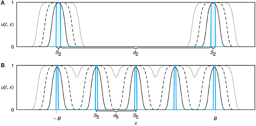
Figure 1. Sketch of the modeled restoration design for a multi-patch set up of n = 2 (A) and n = 5 (B) patches. Initial conditions of planted propagules are shown in cyan. Patches are distributed equidistantly with inter-patch distance d_n. With increasing number of patches we reduce both the patch width S_n, keeping the initial total population size nS_n constant, and the distances between the patches d_n, ensuring that edges of the outer patches remain at the same locations ±B for all configurations. The solid, dashed, and dotted lines show simulated spatial profiles of the growing and expanding population at subsequent time points.

2.2.1. Single-Patch Set-Up

We started by examining the behavior of a single patch of propagules planted at the center of the habitat. Formally, this is the initial condition

where S is the initial width of the patch. Thus, the initial total population size equals P₀ = S. For the simulations of a single patch system we varied the patch widths in the range 0.05 ≤ S ≤ 10 and we used the habitat size of L = 50 throughout.

To evaluate the influence of the initial width S on the development of the patches, we defined the absolute and relative growth rate. The absolute growth rate until time t is

If the absolute growth rate is positive, it describes how much larger the total population has become from the start until time t. If it is negative, it describes how much the population has shrunk until time t. We deliberately chose the slightly cumbersome term “absolute growth rate” to distinguish it from more common notions of growth rate and especially the relative growth rate.

The relative growth rate accounts for the fact that resources are limited in restoration projects due to the initial effort. It divides the absolute growth rate by the initial width (corresponding to the initial population size), that is

For example, if two patches increased by the same amount within a given time frame, the patch with the smaller initial population size (and therefore fewer used resources) would have a higher relative growth rate.

2.2.2. Multi-Patch Set-Up

Next, we generalized our model to a configuration with multiple patches of initial plantings (Figure 1). We designed the planting configuration in such a way that the invested restoration resources (the total initial population size P₀) were fixed and divided equally into n equidistant initial planting patches of width S_n = P₀/n. As a second constraint, in the multi-patch setting we kept the outer borders of the initial restoration region (−B, B) fixed. Single patches (the case n = 1) were placed at the center of the domain as described before. For n ≥ 2, the patches were placed such that the outer edges of the patches furthest left and right were at position x = −B and x = B. Hence, the distance between two patches is always given as $d_n=\frac{2·B-P_0}{n-1}$ and thus, both the initial patch width S_n and the inter-patch distance d_n are decreasing functions of n. This set-up allows to mimic the clumped and dispersed configuration as described in the field experiment by Silliman et al. (2015).

Comparing different numbers of patches n, we denoted the total population size at time t by P_t(n) to emphasize the dependence on the different initial configurations. As parameter values in the multi-patch set-up we used an initial total population size of P₀ = 10 and an initial restoration region of B = 100 throughout, varied the number of patches from n = 1 to n = 15 and increased the total habitat size to L = 250 so that edge effects did not play any role.

Note that the total population size P_t(n), and thus the simulated planting success, always depends on the chosen time horizon t. In order to measure the efficiency of the restoration efforts in a time-independent fashion, we also computed the discounted total population size. Discounting is often used in economics and describes that yields in the future are less valuable than present yields. It is computed in the form of a population-size weighted time integral

Here, ρ is the discounting factor which can be understood as a “negative interest rate”. The larger ρ, the more the population size in the beginning is weighted and the less the population size in the end influences P_ρ(n). The discounted population size only depends on the number n of patches in the initial conditions and thus indirectly on the initial planting distance. We chose ρ = 0.1 and ρ = 0.5. To make the results for the different discounting factors comparable we used the discounted sizes relative to the configuration with one patch, i.e., P_ρ(n)/P_ρ(1).

3. Results

3.1. Single-Patch Set-Up

The spatio-temporal development of a single, newly planted patch is illustrated in Figure 2 for different growth functions and patch widths. In general, we can distinguish three characteristic growth phases: 1. “flattening,” 2. “regrowth,” and 3. “traveling fronts.” In the first (flattening) phase, the diffusion term dominates, outweighing the local growth term f(u) due to the sharp spatial gradient between the patch (representing the initial planting) and the surrounding area (representing the bare substrate). As a consequence, the population density decreases within the patch and increases in the area close to it. In this stage, the population either goes extinct (Ryabov and Blasius, 2008) or it may survive the initial decline. If the planted population does not go extinct it can enter the second and third growth phase. In the second phase (regrowth), the spatial variations equalize and the effect of diffusion is less intense. Consequently, the influence of the local growth function becomes more important, yielding a rising population density. Once the full population density u = 1 is reached again in the center of the patch, a traveling front is established on each side of the patch and the third growth phase is initiated. In this phase, the population spatially expands with nearly constant velocity. This spreading velocity can be analytically described as the asymptotic speed c of a traveling front for each of the three growth functions, yielding $c=\sqrt{2rD}$ for purely logistic growth and $c=\sqrt{2rD}(1/2-a)$ in the presence of an Allee effect (Lewis and Kareiva, 1993; Murray, 1993; Ryabov and Blasius, 2008). Thus, the spatial spreading velocity of the planted population is highest for a population with logistic growth and lowest in the presence of a strong Allee effect.

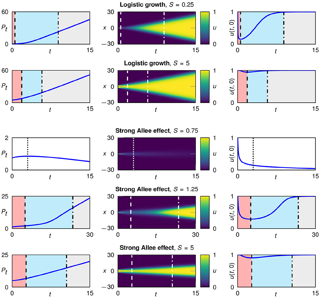
Figure 2. Typical development of a population starting from single patch initial conditions with different widths, for logistic growth f_L(u) (rows 1 and 2) and the strong Allee effect f_A(u) with a = 0.1 (rows 3–5). Plotted are the total population size over time (left), the spatio-temporal development in color coding (middle column) and the population density in the center of the patch (right). In the case of logistic growth the population survives for all patch widths; for the strong Allee effect, populations with a very narrow initial patch go extinct. A surviving population undergoes three characteristic growth phases: 1. flattening (red), 2. regrowth (blue), and 3. traveling fronts (gray).

The initial patch width S plays a central role for the growth dynamics. In particular, the duration of the first and the second growth phase crucially depends on S. The narrower the patch, the stronger is the influence of diffusion on both sides in relation to the whole patch. Consequently, for smaller initial patches the flattening happens faster and the first phase is shorter. Further, the population density in the center of the patch decreases more, leading to a prolonged second phase. This is illustrated in Figure 2, first and second row.

For logistic growth and the weak Allee effect (a = 0) all populations survive the flattening growth phase irrespective of the initial patch width. In contrast, in the case of a strong Allee effect, a minimal initial patch width is needed for survival, while populations on narrow initial patches go extinct (Figure 2, third row). The patches that survive go through the three growth phases (Figure 2, fourth and fifth row). When logistic growth is used or a weak Allee effect is present, the local growth term f(u) is positive as long as the population density u is positive (and smaller than the capacity). Therefore, the strong decrease of the population density in very narrow patches is not critical. If, in contrast, the local growth term includes a strong Allee effect, the growth rate f(u) becomes negative for small population densities. For very narrow patches the population density can then fall below the Allee threshold and consequently the population goes extinct.

In Figure 3, we summarize the simulated population growth rates as a function of the initial patch width S for the three characteristic growth functions. To this end, we computed the absolute and relative growth rates, Equations (5, 6), for a fixed time horizon and analyzed the influence of the initial patch width. For logistic growth, the absolute growth rate g_abs is always positive and approximately equal for all patch widths (Figure 3A). For short time spans, e.g., t = 1, wider patches have higher absolute growth rates than narrower ones but this effect vanishes for longer time horizons. For t = 20, for example, all patches wider than S ≈ 1 have almost equal values of g_abs. Since there is little variation of the absolute growth rates with the patch width, narrower patches have higher relative growth rates (Figure 3D). In terms of restoration efforts, narrow patches thus give a better “return on investment” when logistic growth is assumed.

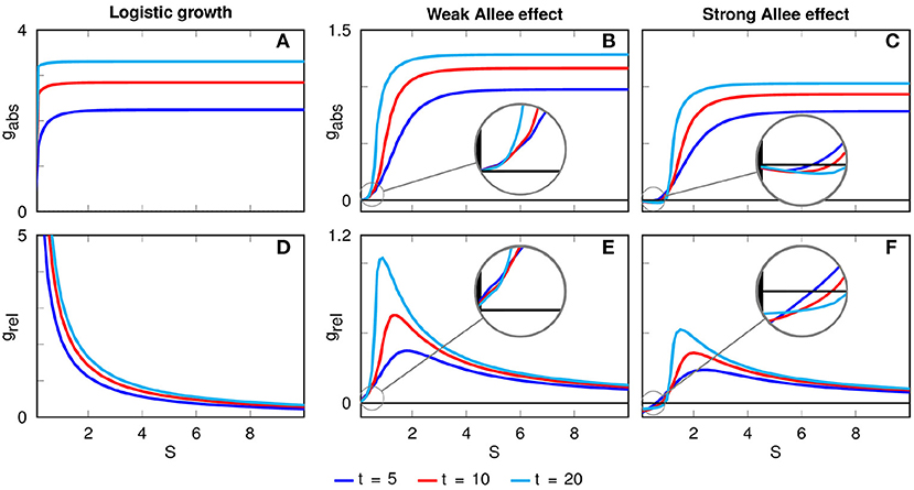
Figure 3. Absolute (A–C) and relative (D–F) growth rates as functions of the patch width S for different time horizons. For logistic growth, the relative growth rate decreases with the initial patch width. In the presence of an Allee effect, there is an optimal patch width of maximal relative growth which depends on the considered time horizon. In the case of a strong Allee effect, the absolute and relative growth rates become negative for very narrow patches, leading to the extinction of the population on those patches.

In the presence of a weak Allee effect, the absolute growth rate is also always positive, but the differences between narrow and wide initial patches are more pronounced than in the case of logistic growth (Figure 3B). Particularly, there is an offset at very small widths before the absolute growth rate rises for intermediate widths and becomes constant for larger widths (Figure 3B). The offset is caused by the shape of the weak Allee effect's growth function (Supplementary Figure 1B): The stronger flattening of very narrow patches leads to small population densities u which have comparatively lower values in the local growth term f(u). Very similar forms of the absolute growth rate are obtained for the case of a strong Allee effect. The main difference is that now g_abs can be negative for small S (Figure 3C), leading to the extinction of populations on very narrow initial patches.

The second row in Figure 3 depicts the dependence of the relative growth rate g_rel on the initial patch width S. While for logistic growth g_rel is always decaying with S, in the case of a weak and strong Allee effect we obtain pronounced peaks of g_rel at intermediate values of S, indicating optimal patch widths. This optimal patch width S_opt depends on the considered time horizon. For example, for the time points t = 5, t = 10 and t = 20 in the case of a weak Allee effect we find S_opt(t = 5) = 1.8, S_opt(t = 10) = 1.3, and S_opt(t = 20) = 0.9, while for a strong Allee effect we obtain S_opt(t = 5) = 2.3, S_opt(t = 10) = 2.0, and S_opt(t = 20) = 1.5. Notice that the optimal width decreases with the time horizon for both weak and strong Allee effect, i.e., when longer time spans are considered narrow patches are recovering and the lower initial effort (that is, the initial patch width) is paying off.

3.2. Multi-Patch Set-Up

The spatio-temporal development of a multi-patch set-up is illustrated in Figure 4 for different growth functions and patch numbers. As in the case of a single-patch set-up, also for a configuration with multiple initial patches the planted population can always survive in a system with logistic growth or weak Allee effect, but may go extinct in the case of a strong Allee effect. This is explained by the fact that the initial width of each patch decays as S_n = P₀/n with the number of patches. We already found in the single-patch set-up that populations do not survive on narrow initial patches when a strong Allee effect is present. This translates into the extinction in configurations with many, and therefore narrow, patches. A main point to keep in mind is that the total initial population size P₀ is fixed. The extinction of configurations with many patches is thus primarily caused by the patch widths S_n being too narrow and is only indirectly linked to the number of patches n.

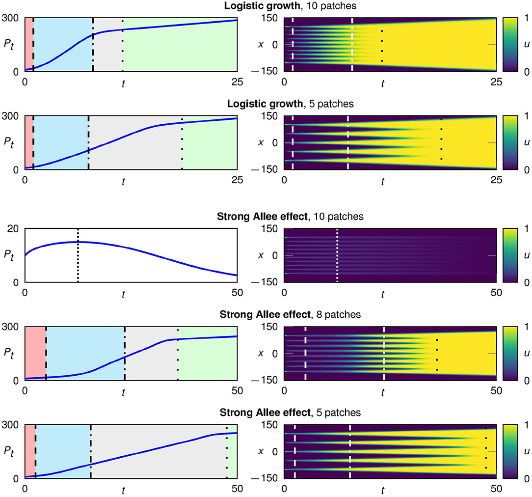
Figure 4. Typical development in configurations starting with multiple initial patches for logistic growth f_L(u) (rows 1 and 2) and the strong Allee effect f_A(u) with a = 0.1 (rows 3–5). We plot the total population size over time (left) and the spatio-temporal development in color coding (right). In the case of logistic growth, the population survives for all spatial configurations. In contrast, for a strong Allee effect, populations starting from a configuration with many and therefore very narrow patches go extinct. A surviving population undergoes four characteristic growth phases: 1. flattening of each patch (red), 2. regrowth of each patch (blue), 3. traveling fronts for each patch (gray), and 4. expansion of the merged patch (green).

As shown in Figure 4, surviving populations go through four growth phases. At the start, the n patches develop separately from each other and we re-encounter the three growth phases 1. “flattening,” 2. “regrowth,” and 3. “traveling fronts” for each patch. In the third growth phase, the system now consists of 2n traveling fronts, which continue to spread until they eventually merge into one big patch with only two fronts remaining. This starts the fourth growth phase “expansion of the merged patch.” Due to the reduction from 2n traveling fronts to only two traveling fronts, after the transition to the fourth growth phase the speed of the population growth, i.e., the changing rate of the total population size P_t(n), is strongly reduced (left column of Figure 4).

Figures 5A–C shows the time dependence of the total population size P_t(n) for several configurations. While all configurations begin with the same initial population size P₀, the total population size as well as the speed of growth start to differ quickly. However, once the patches have merged, the further growth of the total population size P_t is independent of the number of initial patches n. This holds for all three growth functions. For each configuration, the transition into the fourth growth phase is clearly visible as a kink (a sudden change of the graph's slope) in the respective growth curve. Note that due to the different asymptotic propagation speeds of traveling fronts, the time span needed to reach the fourth growth phase differs between the growth functions f(u). For logistic growth, the fronts asymptotically travel faster, hence the merging occurs earlier than for the weak and strong Allee effect.

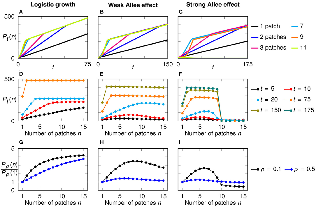
Figure 5. Time dependence and growth dynamics in a configuration with multiple initial patches for logistic growth (left), weak Allee effect (middle), and strong Allee effect (right). (A–C) Temporal development of the total population size for different numbers n of initial patches, with a fixed total initial population size P₀ = 10. A kink in the growth curves indicates the point of merging. (D–F) Total population size after a fixed time horizon in dependence of the number of initial patches. For each model, only time horizons up to the merging of the configuration with two patches are selected. (G–I) Discounted population size relative to the discounted population size for one initial patch in dependence of the number of patches, shown for two discounting rates.

In Figures 5D–F, we plot the total population size P_t(n) as a function of the number of initial patches n at selected time points. Thereby, it becomes transparent that for each growth function f(u) we considered, there are two stages in the growth dynamics: before the merging (short-term behavior) and after the merging (long-term behavior).

We first study the short-term behavior. In the first three growth phases, before the occurrence of any mergings, we can assume that the patches develop separately from each other. Since they all have the same width S_n, they grow with the same speed. Hence the growth of the total population size until time t is n times the absolute growth rate of each patch, that is n·g_abs(S_n, t), with g_abs being the absolute growth rate of a single initial patch (Equation 5). Using the relations g_rel(S_n, t) = g_abs(S_n, t)/S_n and S_n = P₀/n this can be rewritten as P₀ · g_rel(S_n, t). That is, before the merging of the traveling fronts the absolute growth of the multi-patch configuration is proportional to the relative growth rate, Equation (6), of a single patch system.

Assume now that the population follows logistic growth. In the previous section we showed that in a single-patch configuration with logistic growth narrow patches always perform better and have higher relative growth rates, while the absolute growth rate is more or less independent of S (Figures 3A,D). From this we can deduce that multi-patch configurations with a larger number of smaller patches grow faster and initially can achieve higher total population sizes. That is, in a system with logistic growth the total population size P_t(n) should scale with the number of initial patches n for short time horizons (Figure 5D).

This is quite different from the initial growth behavior in the presence of an Allee effect. In this case we found that a single-patch configuration exhibits a pronounced peak of g_rel for intermediate values of S (Figures 3E,F). Thus, for short time spans also a multi-patch system should exhibit highest growth rates for intermediate initial patch sizes and thus intermediate number of patches. This theory is confirmed in the numerical simulations which reveal a unimodal dependency of the total population size P_n(t) as a function of n for time instances before the merger of traveling fronts (Figures 5E,F). The optimal number of patches that maximizes growth rates depends on the time horizon and by comparison with Figures 3E,F indeed is directly related to the optimal patch width derived in the single-patch set-up.

Next we consider the growth behavior for larger time horizons, in the time after the merging of initial patches. In this regime the whole initial restoration region between −B and B is fully populated. Thus, the further growth is only dependent on how far the two outer initial patches have spread. This is measured by the absolute growth rate g_abs(S, t). That is, after the merging of the traveling fronts the absolute growth of the multi-patch configuration is proportional to the absolute growth rate, Equation (5), of a single patch system.

Again, we first assume that the populations follow logistic growth. In Figure 3A, we showed that the absolute growth rate of single patch systems is almost independent of the patch width when t is large. Therefore, the differences between the configurations, that were present for shorter time spans, vanish; all configurations, except the single patch, reach the same total population size (Figure 5D). The lower values for the case n = 1 are explained by the structural disadvantage of a single patch in the center of the simulated area in our chosen initial conditions regarding the long-term behavior: All other configurations start their outwards growth from two sides at x = ±B while the single patch begins at the center.

For the weak and strong Allee effect, the configuration with two patches performs best in the long run (Figures 5E,F) since the absolute growth rate in a single patch system decreases with smaller widths (Figures 3B,C). The decrease of P_t(n) with increasing n for a fixed but large enough time point t is less pronounced for the weak Allee effect than for the strong Allee effect. This is a reflection of the less distinct change in the absolute growth rate for small widths.

Regarding the discounted population size, the most dispersed configuration performs best when using logistic growth while an intermediate number of patches is optimal when an Allee effect is present (Figures 5G–I). These results are in line with the short-term behavior. This is natural since discounting puts more weight on the beginning. While the exact time point t was relevant in the comparison of the total population sizes P_t(n), now the discounting factor ρ determines which configuration is optimal.

4. Discussion

In this study we proposed a simple mathematical model that predicts the success of a plant restoration based on the planting configuration. We consider a standard logistic growth model that inherently includes competitive interactions among individuals and compare this to models that include positive interactions among individuals in which the growth of neighbors promotes the growth and survival of conspecifics. This is integrated into the models in the form of an Allee effect which describes an inverse, density dependence where population growth is positively correlated with density, at least at low population sizes like those found in the beginning of a restoration effort. We found that the optimal planting strategy depends on the type of interactions that take place among individuals, which in turn are related to environmental stress. Thereby, intermediate clumping is likely to maximize plant spread under medium and high stress conditions (high occurrence of Allee effects) while dispersed designs maximize growth under low stress conditions where competitive interactions dominate.

Our results coincide with the findings of a salt-marsh restoration experiment by Silliman et al. (2015). In this experiment only two planting arrangements were compared: the clumped and the dispersed configuration, where the first performed better. In our simulation, the configurations ranged from one wide patch (very clumped) to 15 narrow patches (very dispersed), aiming for a conceptual exploration rather than an exact replication of the experimental results. Our analysis of a model with logistic growth showed that the most dispersed configuration performed best in the short run in contrast to the experimental results. This suggests that positive species interactions, as expressed in our model by an Allee effect, are a crucial component to explain the findings by Silliman et al. (2015). Using simulations that included a weak or strong Allee effect, we found that population growth was optimized for an intermediate number of patches. Further increases in the number of patches, representing more dispersed configurations, only reduced the population growth. This simulation result is in line with the experimental finding that the restoration success was smaller in the dispersed than in the clumped configuration. In our simulations, the most clumped configuration yields the highest population density for short time spans when an Allee effect is present if the initial population size is chosen appropriately (Supplementary Figure 2). Our observation of reduced growth for over-clumped configurations (which was not investigated in the field experiment) can be explained by the fact that spreading of planted patches is only possible from the edges of the patch. Planting designs that were too clumped reduced the number of patches, and thus, the spreading potential.

These results are in line with other studies from the literature, which identified the Allee effect as an important factor for the invasion of plants. For example, Davis et al. (2004) suggested that an Allee effect limits the invasive spread of a salt marsh species and a model by Murphy and Johnson (2015) associated a reduced Allee effect with invasion success. The presence of an Allee effect also drastically changes spreading characteristics of invading species (Gastner et al., 2011). Finally, our results are largely confirmed in a recent field experiment by Duggan-Edwards et al. (2020) who investigated optimal configurations for a salt marsh restoration.

Our findings highlight the importance of positive species interactions for allowing establishment and maximizing population growth from a large number of small initial plantings—a typical configuration in restoration campaigns. The Allee effect expresses the fact that per capita population growth rates are reduced for small population densities. This means that positive interactions from conspecifics are needed to improve survival and reproductive success of an individual or population (Courchamp et al., 1999). This state of a small initial population density and a negative growth rate in the absence of other positive interactions (i.e., high physical stress) is exactly the situation that one should expect for freshly planted populations after restoration. In contrast, competitive interactions should become important only after successful establishment, that is, after the restoration effort already has succeeded. There are many examples for such facilitative mechanisms. In saltmarsh systems, for example, there are positive interactions between vegetation and the surrounding sediments. Plants dissipate wave energy which helps to mitigate wave-induced erosion stress and to shelter from destruction by storm events (Barbier et al., 2011). The reduction of hydrological energy stimulates sediment deposition, enhancing plant survival at higher elevations (Bouma et al., 2009; Silliman et al., 2015; Duggan-Edwards et al., 2020). Further positive interactions between neighboring plants can occur due to alleviation of physical stress due to anoxia. Here the positive feedback is provided in the form or oxygen diffusing from shallow roots into sediments which then becomes available to neighboring plants (Howes et al., 1986).

The Stress Gradient Hypothesis predicts that neighbors are more likely to cooperate with each other as biotic or abiotic stress increases in a system. This theory has been tested in numerous field studies and there is strong support for it as general rule in ecology (He et al., 2013). Although our model did not include stress, we did vary the contribution of positive species interactions by varying the strength of the Allee effect (none, weak, and strong). Given the stress gradient hypothesis, this can be considered as a proxy for environmental stress in the system, with a strong Allee effect signifying high stress and a low Allee effect low stress. With this correlation, we can then make predictions about what type of interactions restoration managers could expect among outplants across a stress gradient and accordingly how to design their planting arrangements to maximize growth rates (Figure 6). Our conceptual study shows that under low stress managers should use fully dispersed planting configurations while under intermediate or high stress, i.e., when when positive interactions likely play a significant role, managers should plant in medium sized clumps. This conclusion is supported by field data for salt-marshes from Silliman et al. (2015) which showed that in the high intertidal, where oxygen is plentiful, plants did better in dispersed than in clumped configurations. However, in the low intertidal, where flooding impedes oxygen diffusing into soil, clumped plants grew 200% more and expanded at greater rates since plants benefited from neighbors oxygenating the soils via translocation of air to their roots. Note that the nature of interactions shifts not only across the stress gradient but also with time. That is, even under conditions of high environmental stress, once a few years have passed, clumps grow into large areas and the foundation species reduces stress—the clones are likely to start to compete more than cooperate. Key then is a new step in restoration planning where managers map out and model stress and intraspecific interactions in their system across the planting zone to determine the optimal mixed method planting design for their area.

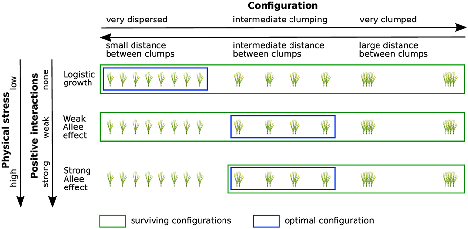
Figure 6. Conceptual visualization of the performance of clumped and dispersed restoration designs in relation to the strength of positive interactions. Green boxes indicate surviving configurations, blue boxes indicate the most efficient method of planting for each growth function. If population dynamics follow logistic growth (no positive interactions) optimal restoration is achieved for a dispersed planting configuration with small distances between clumps. In the presence of an Allee effect optimal performance is obtained for intermediate clumping, while too clumped configurations yield bad restoration performance for all growth functions. According to the Stress Gradient Hypothesis positive interactions (e.g., facilitation) become more significant with increasing physical stress. Thus, although it is not explicitly included into our model, the strength of the Allee effect (none, weak, strong) can be considered as a proxy for physical stress, allowing us to draw conclusions on expected restoration success in different stress regimes.

While we modeled an Allee effect with the specific growth function, f(u) = u(u−a)(1−u) with a = 0 and a = 0.1, we assume that our results generally also hold for other specifications of the weak and strong Allee effect. We were able to explain the behavior for the multi-patch set-up in terms of the dynamics of a single-patch system. Hence, we assume that very narrow patches go extinct for growth functions with negative values for small population densities, i.e., a strong Allee effect. Further, we suggest that there is an optimal patch width, resulting in an optimal number of patches, for all growth functions with smaller per capita growth rates at smaller population densities, i.e., growth functions with an Allee effect, instead of narrower patches always performing better as it is the case for logistic growth.

We investigated a planting configuration where a fixed amount of invested restoration resources is divided equally among the initial planting patches. That is, our simulation design implements an important trade-off where planting in a clumped design will necessarily reduce the spatial extent of the restoration as compared to planting with a dispersed design. The potential costs of doing this must be borne by the growth and spatial spread of the population. On the other hand, cost may be borne primarily in the extent to which ecosystem services are created by the restoration, e.g., if the restored habitat enhances faunal survival or biodiversity. This relates to the more general question of how restoration success is quantified. While our study measures restoration success as the total restored population size, in general, restoration success could be based on the relative magnitude and scale of ecosystem services. This is further complicated by the fact that restoration success also depends on time. Our analysis shows that the total population size reached after restoration varies with the investigated time horizon, depending on the characteristic growth phases shown in Figures 2, 4. In particular, growth dynamics in a multi-patch configuration crucially depend on whether or not the traveling fronts starting from individual patches have already merged (as shown in Figure 5). Thus, also our estimation of the restoration success will depend on the considered time horizon. This raises the question how to equate restoration benefits and ecosystem services that come in the distant future to their value in the present. Here we follow the key paradigm in economics and cost-benefit analysis that future goods should be counted for less than present goods. That is, we discounted future population sizes to present population sizes through the use of a discounting rate, which expresses the intuitive notion that “a dollar today is worth more than a dollar tomorrow.” These ideas from ecological economics are sometimes considered as being in conflict to our desire to have restorations that are sustainable and that persist for more than just the short term. This is a subtle and sometimes controversially discussed issue and we refer the reader to the excellent treatment by Broome (1994).

A diffusive single-species model is of course not a perfect description of the environmental and ecological situations in the restoration of ecosystems. It assumes a homogeneous environment, neglects stochastic events and does not feature interactions with other species, such as grazers or ecosystem engineers (e.g., Lewis and Kareiva, 1993). Additionally, there are many other factors that potentially contribute to restoration success. This includes community level processes, interspecies interactions, environmental change and disturbances, but also possible trade-offs between planting configuration and the potential effects of other species, or the rapidity with which restored habitat is colonized by higher organisms. Planting in a dispersed configuration, for example, can be seen as a form of bet hedging under the expectation of patchy disturbances by (e.g.,) physical disturbances, bioturbation, or herbivory. Consideration of such processes, all of which might be relevant for a real-world restoration scenario, is beyond the scope of this study which applies a simple single-population model for addressing the consequences of different initial plantings.

Considering the above mentioned processes, our study provides interesting new avenues for future model studies, for example, by extending our findings to a community level. Another interesting model extension would be to investigate the effects of non-local species interactions. In our model we assumed that the Allee effect acts only locally, i.e., the growth at point x depends only on the population density at this point. An important next step could be to include a term that measures the population density around each point, for example by using a convolution with a kernel. While most single species models that use a kernel focus on density dependent competition (e.g., Britton, 1989; Han et al., 2016), an interesting extension could be to use such a term to model facilitation and to explore its effect on the behavior of clumped and dispersed initial conditions.

Recently there has been a renewed interest in the application of optimal control theory for spatial ecology and the design of marine reserves (Neubert, 2003; Upmann et al., 2021). Our findings suggest that mathematical modeling and theoretical investigations of optimality might play a similar important role in helping to design optimal configurations and enhance the efficiency of spatial restoration efforts. Even though we used a simple conceptual model, our approach could easily be applied to specific systems and calls for integration of this theory into practice.

Data Availability Statement

The original contributions presented in the study are included in the article/Supplementary Material, further inquiries can be directed to the corresponding author/s.

Author Contributions

BB and BS conceived the study. BB and LH designed the model. LH performed the numerical simulations. All authors contributed to the writing.

Funding

This project was funded by German Research Foundation (DFG) in the Research Unit DynaCom Grant Number FOR 2716. Open access publication fees paid by the Carl von Ossietzky University's open access publication fund.

Conflict of Interest

The authors declare that the research was conducted in the absence of any commercial or financial relationships that could be construed as a potential conflict of interest.

Acknowledgments

We thank Hannes Uecker and Thorsten Upmann for helpful discussions.

Supplementary Material

The Supplementary Material for this article can be found online at: https://www.frontiersin.org/articles/10.3389/fmars.2020.610412/full#supplementary-material

References

Aronson, J., Clewell, A. F., Blignaut, J. N., and Milton, S. J. (2006). Ecological restoration: a new frontier for nature conservation and economics. J. Nat. Conserv. 14, 135–139. doi: 10.1016/j.jnc.2006.05.005
Bakrin Sofawi, A., Rozainah, M. Z., Normaniza, O., and Roslan, H. (2017). Mangrove rehabilitation on carey island, malaysia: an evaluation of replanting techniques and sediment properties. Mar. Biol. Res. 13, 390–401. doi: 10.1080/17451000.2016.1267365
Barbier, E., Hacker, S., Kennedy, C., Koch, E., Stier, A., and Silliman, B. (2011). The value of estuarine and coastal ecosystem services. Ecol. Monogr. 81, 169–193. doi: 10.1890/10-1510.1
Benjamin, C. S., Punongbayan, A. T., dela Cruz, D. W., Villanueva, R. D., Baria, M. V. B., and Yap, H. T. (2017). Use of bayesian analysis with individual-based modeling to project outcomes of coral restoration. Restor. Ecol. 25, 112–122. doi: 10.1111/rec.12395
Bertness, M. D., and Callaway, R. (1994). Positive interactions in communities. Trends Ecol. Evol. 9, 191–193. doi: 10.1016/0169-5347(94)90088-4
Bouma, T. J., Friedrichs, M., Van Wesenbeeck, B. K., Temmerman, S., Graf, G., and Herman, P. M. J. (2009). Density-dependent linkage of scale-dependent feedbacks: a flume study on the intertidal macrophyte spartina anglica. Oikos 118, 260–268. doi: 10.1111/j.1600-0706.2008.16892.x
Britton, N. (1989). Aggregation and the competitive exclusion principle. J. Theor. Biol. 136, 57–66. doi: 10.1016/S0022-5193(89)80189-4
Broome, J. (1994). Discounting the future. Philos. Publ. Affairs 23, 128–156. doi: 10.1111/j.1088-4963.1994.tb00008.x
Courchamp, F., Clutton-Brock, T., and Grenfell, B. (1999). Inverse density dependence and the allee effect. Trends Ecol. Evol. 14, 405–410. doi: 10.1016/S0169-5347(99)01683-3
Davis, H., Taylor, C., Civille, J., and Strong, D. (2004). An allee effect at the front of a plant invasion: spartina in a pacific estuary. J. Ecol. 92, 321–327. doi: 10.1111/j.0022-0477.2004.00873.x
Dobson, A., Bradshaw, A., and Baker, A. (1997). Hopes for the future: restoration ecology and conservation biology. Science 277, 515–522. doi: 10.1126/science.277.5325.515
Duggan-Edwards, M. F., Pagés, J. F., Jenkins, S. R., Bouma, T. J., and Skov, M. W. (2020). External conditions drive optimal planting configurations for salt marsh restoration. J. Appl. Ecol. 57, 619–629. doi: 10.1111/1365-2664.13550
Gastner, M., Oborny, B., Ryabov, A., and Blasius, B. (2011). Changes in the gradient percolation transition caused by an allee effect. Phys. Rev. Lett. 106:128103. doi: 10.1103/PhysRevLett.106.128103
Gedan, K. B., and Silliman, B. R. (2009). Using facilitation theory to enhance mangrove restoration. AMBIO 38:109. doi: 10.1579/0044-7447-38.2.109
Halpern, B., Silliman, B., Olden, J., Bruno, J., and Bertness, M. (2007). Incorporating positive interactions in aquatic restoration and conservation. Front. Ecol. Environ. 5, 153–160. doi: 10.1890/1540-9295(2007)5[153:IPIIAR]2.0.CO;2
Halpern, B. S., Walbridge, S., Selkoe, K. A., Kappel, C. V., Micheli, F., D'Agrosa, C., et al. (2008). A global map of human impact on marine ecosystems. Science 319, 948–952. doi: 10.1126/science.1149345
Han, B.-S., Wang, Z.-C., and Feng, Z. (2016). Traveling waves for the nonlocal diffusive single species model with allee effect. J. Math. Anal. Appl. 443, 243–264. doi: 10.1016/j.jmaa.2016.05.031
He, Q., Bertness, M., and Altieri, A. (2013). Global shifts towards positive species interactions with increasing environmental stress. Ecol. Lett. 16, 695–706. doi: 10.1111/ele.12080
Howes, B., Dacey, J., and Goehringer, D. (1986). Factors controlling the growth form of spartina alterniflora: feedbacks between above-ground production, sediment oxidation, nitrogen and salinity. J. Ecol. 74, 881–898. doi: 10.2307/2260404
Jordan, W., Jordan, W. III, Gilpin, M., and Aber, J. (1990). Restoration Ecology: A Synthetic Approach to Ecological Research. Cambridge: Cambridge University Press.
Leemans, R., and De Groot, R. (2003). Millennium Ecosystem Assessment: Ecosystems and Human Well-Being: A Framework for Assessment. Washington, DC: Island Press.
Lewis, M., and Kareiva, P. (1993). Allee dynamics and the spread of invading organisms. Theor. Popul. Biol. 43, 141–158. doi: 10.1006/tpbi.1993.1007
McCallum, K. P., Breed, M. F., Paton, D. C., and Lowe, A. J. (2019). Clumped planting arrangements improve seed production in a revegetated eucalypt woodland. Restor. Ecol. 27, 638–646. doi: 10.1111/rec.12905
Murphy, J., and Johnson, M. (2015). A theoretical analysis of the allee effect in wind-pollinated cordgrass plant invasions. Theor. Popul. Biol. 106, 14–21. doi: 10.1016/j.tpb.2015.10.004
Neubert, M. G. (2003). Marine reserves and optimal harvesting. Ecol. Lett. 6, 843–849. doi: 10.1046/j.1461-0248.2003.00493.x
Renzi, J., He, Q., and Silliman, B. (2019). Harnessing positive species interactions to enhance coastal wetland restoration. Front. Ecol. Evol. 7:131. doi: 10.3389/fevo.2019.00131
Ryabov, A., and Blasius, B. (2008). Population growth and persistence in a heterogeneous environment: the role of diffusion and advection. Math. Model. Nat. Phenomena 3, 42–86. doi: 10.1051/mmnp:2008064
Silliman, B., Schrack, E., He, Q., Cope, R., Santoni, A., Van Der Heide, T., et al. (2015). Facilitation shifts paradigms and can amplify coastal restoration efforts. Proc. Natl. Acad. Sci. U.S.A. 112, 14295–14300. doi: 10.1073/pnas.1515297112
Silliman, B. R., and He, Q. (2018). Physical stress, consumer control, and new theory in ecology. Trends Ecol. Evol. 33, 492–503. doi: 10.1016/j.tree.2018.04.015
Sleeman, J., Boggs, G., Radford, B., and Kendrick, G. (2005). Using agent-based models to aid reef restoration: Enhancing coral cover and topographic complexity through the spatial arrangement of coral transplants. Restor. Ecol. 13, 685–694. doi: 10.1111/j.1526-100X.2005.00087.x
Stachowicz, J. (2001). Mutualism, facilitation, and the structure of ecological communities. BioScience 51, 235–246. doi: 10.1641/0006-3568(2001)051[0235:MFATSO]2.0.CO;2
Suding, K. (2011). Toward an era of restoration in ecology: successes, failures, and opportunities ahead. Annu. Rev. Ecol. Evol. Syst. 42, 465–487. doi: 10.1146/annurev-ecolsys-102710-145115
Upmann, T., Uecker, H., Hammann, L., and Blasius, B. (2021). Optimal stock-enhancement of a spatially distributed renewable resource. J. Econ. Dyn. Control. 123:104060. doi: 10.1016/j.jedc.2020.104060
Valdez, S. R., Zhang, Y. S., van der Heide, T., Vanderklift, M. A., Tarquinio, F., Orth, R. J., et al. (2020). Positive ecological interactions and the success of seagrass restoration. Front. Mar. Sci. 7:91. doi: 10.3389/fmars.2020.00091
Worm, B., Barbier, E., Beaumont, N., Duffy, J., Folke, C., Halpern, B., et al. (2006). Impacts of biodiversity loss on ocean ecosystem services. Science 314, 787–790. doi: 10.1126/science.1132294
Young, T. (2000). Restoration ecology and conservation biology. Biol. Conserv. 92, 73–83. doi: 10.1016/S0006-3207(99)00057-9
Young, T., Petersen, D., and Clary, J. (2005). The ecology of restoration: historical links, emerging issues and unexplored realms. Ecol. Lett. 8, 662–673. doi: 10.1111/j.1461-0248.2005.00764.x
Keywords: restoration, restoration design, optimality, Allee effect, diffusion, mathematical modeling, coastal wetlands
Citation: Hammann L, Silliman B and Blasius B (2021) Optimal Planting Distance in a Simple Model of Habitat Restoration With an Allee Effect. Front. Mar. Sci. 7:610412. doi: 10.3389/fmars.2020.610412
Received: 25 September 2020; Accepted: 28 December 2020;
Published: 22 January 2021.
Edited by:
Romuald Lipcius, College of William & Mary, United StatesReviewed by:
Kevin Alexander Hovel, San Diego State University, United StatesJunping Shi, College of William & Mary, United States
Copyright © 2021 Hammann, Silliman and Blasius. This is an open-access article distributed under the terms of the Creative Commons Attribution License (CC BY). The use, distribution or reproduction in other forums is permitted, provided the original author(s) and the copyright owner(s) are credited and that the original publication in this journal is cited, in accordance with accepted academic practice. No use, distribution or reproduction is permitted which does not comply with these terms.
*Correspondence: Liv Hammann, liv.tatjana.hammann@alum.uni-oldenburg.de; Bernd Blasius, blasius@icbm.de