Dynamics and Origin of Transparent Exopolymer Particles in the Oyashio Region of the Western Subarctic Pacific during the Spring Diatom Bloom
 Yuichi Nosaka
 Youhei Yamashita
 Koji Suzuki
- 1Graduate School of Environmental Science, Hokkaido University, Sapporo, Japan
- 2Faculty of Environmental Earth Science, Hokkaido University, Sapporo, Japan
- 3JST-CREST, Sapporo, Japan
The seasonal biological drawdown of the partial pressure of CO2 (pCO2) in the surface waters of the Oyashio region of the western subarctic Pacific is one of the greatest among the world's oceans. This is attributable to spring diatom blooms. Transparent exopolymer particles (TEPs) are known to affect efficiency of the biological carbon pump, and higher TEP levels are frequently associated with massive diatom blooms. However, TEP dynamics in the Oyashio region remain unclear. We investigated the TEP distribution from three cruises during the spring diatom bloom periods in 2010 and 2011. TEP concentrations varied from <15 to 196 ± 71 μg xanthan gum equiv. L−1 above 300 m and generally declined with depth. Vertical TEP concentrations were significantly related not only to chlorophyll a concentrations but also to bacterial abundance. Average TEP concentrations within the mixed layer (>30 m) were significantly higher during the bloom (155 ± 12 μg xanthan gum equiv. L−1) than in the post-bloom phase (90 ± 32 μg xanthan gum equiv. L−1). In contrast, bacteria abundance within the mixed layer changed little during the bloom to post-bloom phases. These results suggest that the abundance of phytoplankton greatly contributed to dynamics of the TEP distribution. To evaluate the ability of the phytoplankton to produce TEP, an axenic strain of the diatom Thalassiosira nordenskioeldii, which is a representative species of Oyashio blooms, was examined within a batch culture system. Cell abundance-normalized TEP and dissolved organic carbon (DOC) production rates changed simultaneously with growth of the strain. Although these production rates were significantly higher in the stationary phase than in the exponential growth period, values of the TEP/DOC ratio changed little throughout incubation. These findings suggest that TEP production in the Oyashio region may be enhanced by an increase in DOC production from spring diatoms.
Introduction
Transparent exopolymer particles (TEPs) are defined as > 0.4-μm transparent particles that consist of acidic polysaccharides, and are stainable with the dye Alcian blue (Alldredge et al., 1993). These particles are very sticky, so that they can facilitate the aggregation of particles in seawater (e.g., Passow, 2002a; Wurl et al., 2011; Mari et al., 2017). Generally, the presence of TEP may increase the efficiency of the biological carbon pump, because TEP-attached particles sink readily (e.g., Passow, 2002a; Wurl et al., 2011). In contrast, TEPs can decrease the sinking rates of aggregates, because the density of TEPs is lower than that of seawater (Azetsu-Scott and Passow, 2004; Mari et al., 2017). TEPs also can be consumed by heterotrophic organisms, such as bacteria, zooplankton, and fish (e.g., Grossart et al., 1998, 2006; Prieto et al., 2001), indicating that the particles are important in marine food webs. It is known that many marine organisms, including phytoplankton and bacteria, can generate extracellular polysaccharides such as TEPs (Passow, 2002a). However, TEPs and their precursors in seawater can be utilized as organic substrates by heterotrophic organisms (Passow, 2002a). TEP levels in the world's oceans are highly variable (0–14,800 μg xanthan gum equivalent L−1; e.g., Hong et al., 1997; Radić et al., 2005). Higher TEP levels are sometimes associated with blooms of phytoplankton, such as diatoms (e.g., Passow et al., 1995), Phaeocystis spp. (e.g., Hong et al., 1997), dinoflagellates (e.g., Berman and Viner-Mozzini, 2001), cryptophytes (e.g., Passow et al., 1995), and cyanobacteria (e.g., Grossart and Simon, 1997). In particular, diatoms are known to excrete large amounts of polysaccharides, which can form TEPs during their actively growing and/or senescent phases (Mari and Burd, 1998; Passow, 2002b). Using batch cultures, Passow (2002b) reported that TEP production varied widely among phytoplankton species. Fukao et al. (2010) showed that TEP productivity of the diatom Coscinodiscus granii was greater in the exponential growth phase than in stationary and decline periods, whereas those of diatoms Eucampia zodiacus, Rhizosolenia setigera, and Skeletonema sp. were greater in the stationary growth and decline phases than in the exponential growth period. To our knowledge, the relationship between the physiology of diatoms and TEP production remains poorly understood.
In the Oyashio region of the Northwest Pacific, massive diatom blooms occur during spring (e.g., Kasai et al., 1998; Saito et al., 2002; Suzuki et al., 2011). These blooms are generally triggered by water-column stratification during the transition from winter to spring (Kasai et al., 1997). The chlorophyll (Chl) a concentration and primary production integrated within the water column can reach 500 mg Chl a m−2 (Kasai et al., 1998) and 3,200 mg C m−2 d−1 (Isada et al., 2010), respectively. The enormous spring blooms cause an increase in meso- and macro-zooplankton biomass and fishery production in the Northwest Pacific (Sakurai, 2007; Ikeda et al., 2008). Takahashi et al. (2002) reported that the Northwest Pacific including the Oyashio is one of the regions where the seasonal drawdown effect of pCO2 by marine organisms is maximized. This is mainly caused by spring diatom blooms (Midorikawa et al., 2003; Ayers and Lozier, 2012). Honda (2003) reported that among the world's oceans, efficiency of the biological carbon pump was relatively high in the Northwest Pacific. Hence, it can be inferred that the relatively high flux of settling particles in the Northwest Pacific is caused by vigorous primary production of diatoms that aggregate and sink. However, TEP dynamics in the Oyashio region during the spring diatom blooms are still poorly understood, even though they are pivotal in biogeochemical and ecological processes.
The main aims of this study were to understand TEP dynamics in the Oyashio region during the spring diatom bloom periods of 2010 and 2011 and to evaluate the relationship between TEP and other parameters. Those parameters include particulate organic carbon (POC) and dissolved organic carbon (DOC) concentrations, POC and DOC production, and phytoplankton and bacterial abundance. In addition, to understand TEP productivity in greater detail, we examined the characteristics of TEP production of an axenic strain of the Oyashio diatom Thalassiosira nordenskioeldii, which is a representative species of spring blooms (Chiba et al., 2004; Suzuki et al., 2011). This was grown in a batch culture system. The importance of TEP production by this strain was assessed.
Materials and Methods
Research Cruises
Three field campaigns were conducted, 13–23 April 2010, 7–16 June 2010, and 5–13 May 2011 (Figure 1). The FR/V Wakataka-Maru (Fisheries Research Agency of Japan) and R/V Tansei-Maru (JAMSTEC/AORI, University of Tokyo) were used for two cruises in 2010 and a single cruise in 2011, respectively. In April, June, and May, two (A1 and A2), four (J1, J2, J3, and J4) and three (M1, M2, and M3) sampling stations were visited, respectively. In all cruises, incident photosynthetic available radiation (PAR) above the sea surface was continuously measured on deck with a PAR sensor (ML-020P, EKO Instruments Co., Ltd., Japan) every 10 min on average, and values were recorded with a data logger. Seawater sampling at all stations was accomplished using a CTD-CMS equipped with acid-clean Niskin bottles. The samples were corrected from 5, 10, 20, 40, 60, 80, 100, 200, and 300 m depths in April 2010, and from the those depths plus 30, 50, and 150 m layers in June 2010 and May 2011. Nutrients (nitrite plus nitrate, hereafter referred to as nitrate, phosphate, and silicate) were determined with a BRAN + LUEBBE auto-analyzer following manufacturer protocol. Basal depth of the mixed layer was defined as a threshold value of temperature or density from a near-surface value at 10-m depth (ΔT = 0.2°C or Δσθ = 0.03 kg m−3; Montégut et al., 2004).
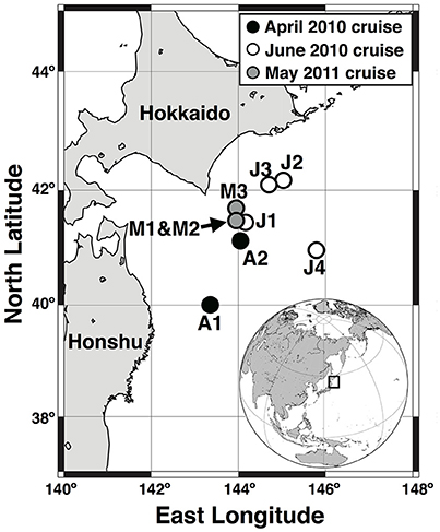
Figure 1. Sampling stations during cruises of April and June 2010 and May 2011, in Oyashio region of western subarctic Pacific.
Phytoplankton Pigments and CHEMTAX Processing
Phytoplankton pigments were analyzed using high-performance liquid chromatography (HPLC). Water samples (500 mL) collected from 5 to 300 m depths were filtered on 25-mm Whatman GF/F filters under a gentle vacuum (< 0.013 MPa). The filter samples were folded, blotted with filter paper, and stored at −80°C. Phytoplankton pigments were extracted with sonication in N, N-dimethylformamide (DMF) according to the protocol of Suzuki et al. (2005). HPLC pigment was analyzed according to the method of Van Heukelem and Thomas (2001), except that the flow rate was 1.2 mL min−1. Details of the analysis method are in Suzuki et al. (2014).
To estimate the contribution of each algal group in the two layers (5–20 and 30–50 m depths) to total Chl a biomass, the pigment data were interpreted by factorization using the CHEMTAX program (Mackey et al., 1996). The initial and final pigment ratios were calculated following the method of Latasa (2007) (Supplementary Table 1). Initial ratios were based on Suzuki et al. (2002, 2005, 2009), who estimated the community composition of phytoplankton in the northwestern Pacific. Prymnesiophytes, pelagophytes, and prasinophytes in our CHEMTAX analysis are synonymous with type 3 haptophytes, type 2 chrysophytes, and type 3 prasinophytes according to Mackey et al. (1996), respectively. Chl a biomass of each algal group was calculated by multiplying in situ Chl a concentrations by the CHEMTAX outputs.
To confirm the development and decline in Chl a concentration from spring to summer, we also examined monthly satellite images of that concentration as observed by a MODIS/Aqua satellite sensor. MODIS/Aqua monthly Chl a data (4-km resolution, OC3M algorithm) for the period February–July 2010 and 2011 were obtained from the Distributed Active Archive Center (DAAC)/Goddard Space Flight Center (GSFC), NASA (http://oceancolor.gsfc.nasa.gov/cgi/l3).
Identification and Cell Abundance of Phytoplankton
Water samples (500 mL) were taken at 5-m depth to count diatoms and coccolithophores, and these samples were fixed with buffered formalin (pH 7.8, 1% final concentration). An aliquot (3–11 mL) of the sample was filtered onto a Nuclepore membrane (1-μm pore size) filter set in a glass funnel (3-mm in diameter at the base) in a vacuum (0.013–0.026 MPa). The filter membrane was rinsed with Milli-Q water to remove salts and immediately dried for 3 h in an oven at 60°C. To identify and count the algal cells, the entire area of the membrane (~7 mm2) was examined by a scanning electron microscope (SEM, VE-8800, Keyence Corp., Japan) at magnification approximately 2,000 ×. Phytoplankton species were identified according to Fukuyo et al. (1990); Tomas et al. (1997), Young et al. (2003), Scott and Marchant (2005), and Round et al. (2007). In our study, the dominant diatom species were defined such that they contributed > 25% to total diatom abundance.
Abundance of Heterotrophic Bacteria
Duplicate water samples (each 2 mL) from 5 to 300 m depths were preserved with paraformaldehyde (0.2% final concentration) and stored at −80°C until analysis on land. An EPICS flow cytometer (XL ADC system, Beckman Coulter, Inc., USA) equipped with a 15-mW air-cooled argon laser exciting at 488 nm and a standard filter setup were used for enumeration of heterotrophic bacteria. Prior to analysis, samples were thawed and drawn through a 35-μm, nylon-mesh-capped Falcon cell strainer (Becton-Dickinson) to remove larger cells. Cells were stained with the nucleic acid stain SYBR Gold solution (Invitrogen). The stock SYBR Gold stain (104-fold concentrations in the commercial solution) was diluted to 10-fold concentrations with Milli-Q water. Twenty-five microliters of the 10-fold SYBR Gold stain was added to the 225-μL bacteria sub-sample and incubated in the dark at room temperature (25°C) for 30 min prior to analysis. The incubated samples were mixed with 250 μL of Flow-Count fluorophores (Beckman Coulter) and then analyzed. Details of the flow cytometric analysis are given in Suzuki et al. (2005).
Particulate Organic Carbon (POC) Concentration
The POC concentration was determined only for the 5-m depth. The 300-mL water sample was filtered onto pre-combusted Whatman GF/F filters (25-mm in diameter, 450°C for 5 h) under a gentle vacuum (< 0.013 MPa) and stored at −20°C until analysis. On land, the samples were thawed at room temperature, exposed to HCl fumes to remove inorganic carbon, and completely dried in a vacuum desiccator for > 24 h. The POC concentrations on the filters were determined with an online elemental analyzer (FlashEA1112, Thermo Fisher Scientific, Inc., USA).
Dissolved Organic Carbon (DOC) Concentration
Samples of DOC were collected from 12 depths between 5 and 300 m. Inline filter holders (PP-47, Advantec MFS, Inc., USA) and tubes (Tygon R-3603, United States Plastic Corp., USA) were pre-cleaned by soaking in 1 M HCl and then rinsed with Milli-Q water. Before sampling, pre-combusted Whatman GF/F filters (47 mm diameter) were set in the inline filter holders, and the tubes were mounted. The water samples were taken by connecting the tube with the spigot of the Niskin bottle. At the start of sampling, filtrates were well drained to pre-wash the tubing, filter holder and filter. Afterward, triplicate samples were collected in pre-combusted 24-mL screw vials with acid-cleaned PTFE septum caps. The samples were immediately stored at −20°C until analysis on land. The frozen samples were thawed and well mixed. DOC concentrations were determined with a total organic carbon analyzer (TOC-V CSH, Shimadzu Corp., Japan). The accuracy and variance of the measured DOC concentrations were checked by analyzing deep seawater reference material provided from the consensus reference material (CRM) program (Prof. Dennis Hansell, University of Miami).
Daily POC and DOC Production
Daily POC and DOC production were estimated using a simulated in situ incubation technique at 5-m depth, except at Station M3 during the May 2011 field campaign. The samples were dispensed into three 300-mL, acid-cleaned polycarbonate bottles (two light and one dark) and inoculated with a solution of NaH13CO3 (99 atom% 13C), equivalent to ~10% of total inorganic carbon (TIC) in the seawater. All bottles were incubated for ~24 h. The incubated POC samples were filtered onto pre-combusted Whatman GF/F filters (25 mm in diameter, 450°C for 5 h) with a gentle vacuum (< 0.013 MPa), and the filtrate was collected in pre-combusted, 500-mL glass bottles (450°C for 5 h). The filter and water samples were stored at −20°C until analysis.
The filter samples of POC production were thawed at room temperature, exposed to HCl fumes to remove inorganic carbon, and then completely dried in a vacuum desiccator for > 24 h. POC concentrations on the filters and 13C abundance were determined using a mass spectrometer (DELTA V, Thermo Fisher Scientific, Inc., USA) with online elemental analyzer (FlashEA1112, Thermo Fisher Scientific). Daily primary production was calculated according to Equation (1) (Hama et al., 1983):
where ais is the 13C atom% in an incubated sample, ans is the 13C atom% in a natural (i.e., non-incubated) sample, aic is the 13C atom% in inorganic carbon, [Cp] is the concentration of POC in the incubated sample, t is the incubation duration (day), and f is the discrimination factor of 13C (i.e., 1.025). In our study, TIC concentrations were determined with a total alkalinity analyzer (ATT-05, Kimoto Electric Co., Ltd., Japan).
DOC production was estimated according to Hama and Yanagi (2001) with a few modifications. The frozen samples were thawed at room temperature (25°C) and were desalinated using an electro dialyzer (Micro Acilyzer S3, ASTOM Corp., Japan) equipped with AC-220-550 cartridge (CMX-SB/AMX-SB, ASTOM Corp., Japan). Conductivity of the water samples decreased from ~53 to 3.0 mS cm−1 within 2–3 h. Before and after desalination, the DOC concentrations were examined. The recovery percentage of those concentrations ranged from 62 to 96%, whereas the conductivity decreased to 6% of the initial value (Supplementary Table 2). The desalinated seawater samples were concentrated to ~5 mL with a rotary evaporator at 45°C using a pre-combusted 500-mL eggplant-shaped flask. HCl was added to the concentrated 5-mL samples to reduce the pH to 2. The low-pH concentrates were purged with N2 gas for ~9 min to remove dissolved inorganic 13C. Thereafter, the samples were further concentrated to ~0.5–1 mL with a rotary evaporator at 45°C using a pre-combusted 10-mL pear-shaped flask. The 13C atom% of DOC absorbed onto the Whatman GF/F filters combusted in a muffle furnace (450°C, 5 h) were determined using a mass spectrometer (DELTA V, Thermo Fisher Scientific) with an online elemental analyzer (FlashEA1112, Thermo Fisher Scientific). Daily DOC production was calculated according to Equation (2) (Hama and Yanagi, 2001):
where [Cd] is the DOC concentration (mg m−3).
Furthermore, we estimated the ratio (PER) of DOC production/total production by phytoplankton according to
Transparent Exopolymer Particle (TEP) Analysis
Water samples of TEP were taken from depths 5–300 m. Triplicate water samples of 250 mL were filtered using Whatman 0.4-μm Nuclepore filters, applying a gentle vacuum (< 0.013 MPa). TEPs captured by the filter were stained with Alcian blue solution (Passow and Alldredge, 1995). The stained filters were immediately rinsed with Milli-Q water and then stored at −20°C until analysis on land.
For the standard TEP curve, the method of Claquin et al. (2008) was modified. As reported by Claquin et al. (2008), the standard curve described in Passow and Alldredge (1995) is applicable only for low concentrations of TEP (i.e., calibration standard weight of xanthan gum ranging between 0 and 40 μg). One milligram of xanthan gum was put into a 15-mL centrifugal tube and added to 10 mL of the Alcian blue stain. The tube was shaken well for ~1 h to combine the xanthan gum and Alcian blue. Thereafter, it was centrifuged at 3,200 × g for 20 min, and the supernatant liquid was carefully removed using micro pipets. Ethanol (99.5%) was added to the tube, which was then centrifuged, and the supernatant liquid was removed via the ethanol precipitation method. The ethanol precipitation was repeated at least five times until the solution became transparent. Finally, as much of the ethanol in the tube as possible was removed. To dry the blue-stained xanthan gum, N2 gas was gently sprayed into the tube. Subsequently, the xanthan gum was completely dried in a desiccator under vacuum for more than 24 h. The blue-stained xanthan gum was dissolved with 6 mL of 80% H2SO4 using a volumetric pipette (stock solution of 1 mg xanthan gum 6-mL−1). The stock solution was diluted with 80% H2SO4, to make a dilution series with five concentrations (10, 50, 100, 150, and 200 μg xanthan gum 6-mL−1). Absorption at 787 nm was measured with a Shimadzu spectrophotometer (MPS-2400) in 1-cm cuvettes, with reference to Milli-Q water. Four slopes of the TEP standard curve were compared with those of Passow and Alldredge (1995) and Claquin et al. (2008) (Supplementary Table 3). Also we conducted a comparison between the standard curves made with this centrifugation and conventional filtration (Passow and Alldredge, 1995) methods. The comparison revealed that the slope (136) of the centrifugation method was lower than that (207) of the conventional method (Supplementary Figure 1). Hence, all TEP concentrations in this study were corrected by multiplying a factor of 1.52. Passow and Alldredge reported that average absorption of the filter blank with 0.4-μm polycarbonate filters was between 0.07 and 0.09. In our study, the filter blank (average ± standard deviation) was 0.081 ± 0.003 (n = 4).
The natural filter samples were transferred into 20-mL vials. Six milliliters of 80% H2SO4 was added to the vials, and the filters were soaked for 2 h. The vials were gently agitated five times over this period. Absorption at 787 nm was measured with the spectrophotometer in 1-cm cuvettes against Milli-Q water as reference. The TEP levels (μg xanthan gum equivalent L−1) were determined according to Passow and Alldredge (1995).
TEP Production by the Oyashio Diatom Thalassiosira nordenskioeldii
A single cell of T. nordenskioeldii Cleve was isolated from Oyashio waters during the May 2011 field campaign. The strain was sterilized in f/2 medium (Guillard and Ryther, 1962; Guillard, 1975) with penicillin and streptomycin (25 U mL−1 of penicillin and 25 μg mL−1 of streptomycin, 17-603E, Lonza Group Ltd., Switzerland) following the methods of Sugimoto et al. (2007). For the culture experiment, salinity of the medium was adjusted to 33.0, which is a typical value of surface Oyasho waters in spring (e.g., Hattori-Saito et al., 2010). Initial nutrient levels in the medium were also modified from f/2 medium to mimic Oyashio water: 20 μM NaNO3, 35 μM Na2SiO3· 9H2O, 2.0 μM NaH2PO4· H2O, 600 nM FeCl3· 6H2O, 600 μM Na2EDTA · 2H2O, 46.7 nM MnCl · 4H2O, 3.9 nM ZnSO4· 7H2O, 2.2 nM CoCl2· 6H2O, 2.0 nM CuCO4· 5H2O, 1.3 nM Na2MoO4· 2H2O, 15 nM Thiamine · HCl, 100 pM Biotin, 19 pM Cyanocobalamin. The axenic strain was inoculated in the medium and grown for ~30 generations in an incubator (MIR-554, Sanyo Electric Co., Ltd., Japan) at 5°C, under 100 μmol photons m−2 s−1 from white fluorescent lamps (FL20SS · BRN/18, Toshiba) with a light-dark cycle of 12 h. At the start of this experiment, the well-acclimated axenic strain was inoculated in Oyashio-simulated medium (17 L) in two acid-cleaned 20-L culture vessels (P/N 2600-0012, Thermo Fisher Scientific) and cultured for 40 days.
Nutrient, Cell Abundance, and Chl a Measurements in the Culture Experiment
Nutrients were sampled every other day. Duplicate water samples per culture vessel were dispensed into acrylic tubes with screw caps, and the samples were immediately stored at −20°C. The frozen samples were thawed at room temperature and well mixed. The nutrient concentrations (nitrate, phosphate, and silicate) were determined with an auto-analyzer (QuAAtro 2-HR, BLTEC Corp., Japan) as described above. Sampling of cell abundance was done every other day. Ten to fifty milliliters of the water samples were transferred into 15 or 50-mL centrifuge tubes. During days 0–14, T. nordenskioeldii was filtered using a 25-mm Whatman Nuclepore membrane filter of 1.0-μm pore size and was immediately resuspended in the non-concentrated water samples. One point five milliliters of the concentrated sample (days 0–14) or non-concentrated sample (days 16–40) was transferred to a micro-slide glass chamber of thickness 1.1 mm (S109502, Matsunami Glass Ind., Ltd., Japan), and covered with a cover glass. To estimate cell abundance, duplicate samples were observed per culture vessel using an epifluorescence microscope (BZ-9000, Keyence Corp., Japan) equipped with a GFP optical filter (OP-66835 BZ filter GFP, Keyence Corp., Japan). The Chl a-derived fluorescence in T. nordenskioeldii was automatically photographed with 28 photos and 4 × magnification, and the fluorescence was summed using image analysis software (Keyence Corp., Japan). Therefore, cell abundance was estimated by dividing the observed volume (mL) by the total value of fluorescence. The specific daily growth rate (μ, d−1) during the culture experiment was estimated by the method of Guillard (1973):
where N0 is initial cell abundance (cells mL−1), Nt the abundance after t days, t0 the initial time (d), and tt the time after t days.
Chl a concentrations were determined in the mid-exponential phase. Triplicate samples per vessel (each 200 mL) were filtered onto Whatman GF/F filters with a gentle vacuum (< 0.013 MPa). The filters were folded, blotted with filter paper, and stored at −80°C. The pigment analysis is described in Section Phytoplankton Pigments and CHEMTAX Processing.
TEP Measurement in the Culture Experiment
TEP was sampled once every 4 days between days 0 and 36. Triplicate water samples (1–20 mL) per culture vessel were filtered using Whatman 0.4-μm Nuclepore membrane filters in a gentle vacuum (< 0.013 MPa). Post-treatment used the same method described in Section Transparent Exopolymer Particle (TEP) Analysis.
DOC Determination in the Culture Experiment
DOC was sampled once every 4 days between days 0 and 36. A filter funnel (25-mm in diameter, PN 4203, PALL Corp., USA) was pre-cleaned by soaking in 1 M HCl, and then rinsed with Milli-Q water. Pre-combusted Whatman GF/F filters were placed in the filter funnel, which was equipped with a suction vessel. The water sample was filtrated in a gentle vacuum (< 0.013 MPa). At the start of sampling, a few milliliters of the filtrates were drained to prewash the GF/F filter and filter funnel. Then, duplicate samples were collected in pre-combusted 24-mL screw vials with acid-cleaned PTFE septum caps. The samples were immediately stored at −20°C until analysis. The analysis method was described in Section Dissolved Organic Carbon (DOC) Concentration.
Daily TEP and DOC Productivities
Based on TEP or DOC concentration in the culture vessels, cellular TEP productivity [pg xanthan gum equiv. (cell)−1 d−1] and DOC productivity [pg C (cell)−1 d−1] averaged during the exponential growth and stationary phases (initial and final) using two data points of those phases were estimated via
where C0 is TEP concentration (pg xanthan gum equiv. mL−1) or DOC concentration (pg C mL−1) at the initial time of the exponential growth phase or stationary phase, Ct is concentration of the TEP or DOC at the final time after t days, t0 is the initial time (d) of the exponential growth phase or stationary phase, tt is the final time after t days, N0 is initial cell abundance (cells mL−1) of the exponential growth or stationary phase, and Nt is cell abundance at the final time after t days. Carbon-based TEP productivity was estimated by multiplying TEP productivity by a factor of 0.75 (Engel and Passow, 2001).
Results
TEP Observations during the Oyashio Spring Diatom Bloom
Hydrography
Seawater temperatures at 5 m increased from April through June 2010 (Table 1). By contrast, salinity only changed slightly throughout the cruises (32.8–33.3). Relatively high nutrient levels were found in April 2010, which declined in June. The surface mixed layer was above 30 m at stations A2, M1, and M2, whereas it was shallower than 10 m at the other stations.
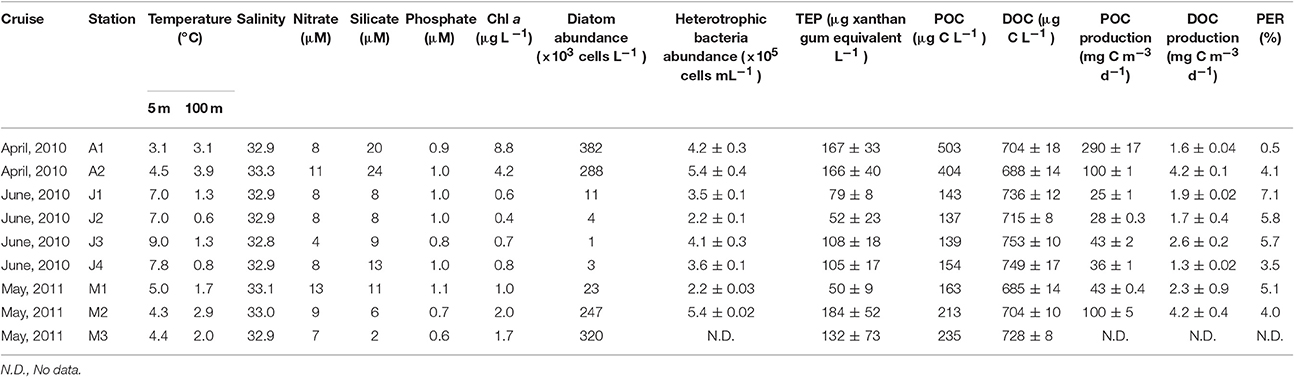
Table 1. Hydrographic conditions and phytoplankton productivity at 5 m depth during Oyashio spring diatom blooms in April and June 2010 and May 2011.
Chlorophyll a Concentrations and Community Composition as Estimated from the CHEMTAX Program
Chl a concentrations generally decreased from April through June 2010 and from 5 to 300 m depths (Figures 2A–C). Satellite surface Chl a images also indicated that decreases in the algal pigment concentration from April to June in 2010 and 2011 (Supplementary Figure 2). The highest Chl a concentration at 5-m depth was observed at station A1 in April 2010 (8.8 μg L−1), whereas the lowest was at station J2 in June 2010 (0.4 μg L−1) (Table 1). Chl a within the mixed layer significantly decreased from April to June (Kruskal-Wallis ANOVA, p < 0.01, Steel-Dwass test, April vs. May: p < 0.01; April vs. June: p < 0.01; May vs. June: p < 0.01).
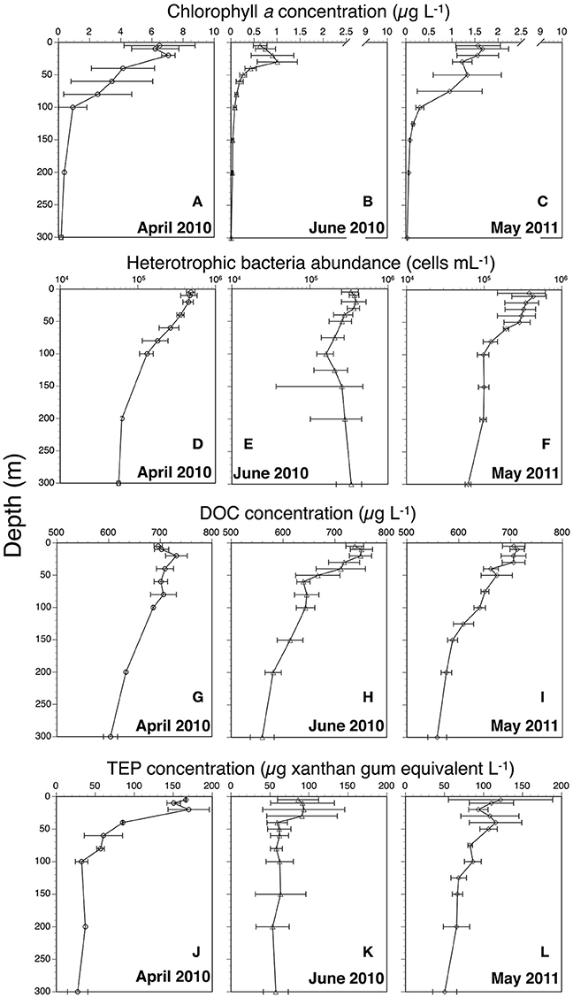
Figure 2. Vertical profiles of chlorophyll a (A: April 2010; B: June 2010; C: May 2011), heterotrophic bacteria abundance (D: April 2010; E: June 2010; F: May 2011), dissolved organic carbon (DOC) (G: April 2010; H: June 2010; I: May 2011), and transparent exopolymer particles (TEP) (J: April 2010; K: June 2010; L: May 2011). All profiles show average values. Error bars represent range for April 2010 (n = 2) and standard deviation for June 2010 (n = 4) and May 2011 (n = 3).
The final ratio matrix in the 5–20 m layer estimated with the CHEMTAX program (Supplementary Table 1B) was within the range of Mackey et al. (1996), except for the alloxanthin:Chl a ratio (0.25), which was slightly larger than that of the maximum (0.23) of Mackey et al. The final ratio matrix in the 30–50 m layer (Supplementary Table 1D) was within the range of Mackey et al. The contributions of each phytoplankton group to Chl a biomass from 5 to 50 m depths are shown in Figure 3. Diatoms dominated in both April 2010 (average ± standard deviation: 94 ± 4%) and May 2011 (80 ± 9%). By contrast, the contributions in June 2010 (35 ± 23%) were relatively small. The contributions of the other phytoplankton groups, such as cryptophytes (20 ± 17%), prasinophytes (19 ± 10%) and prymnesiophytes (9 ± 6%), were larger than those in April 2010 (cryptophytes: 1 ± 2%; prasinophytes: 2 ± 2%; prymnesiophytes: 0.4 ± 0.5%) and May 2011 (cryptophytes: 9 ± 5%; prasinophytes: 3 ± 2%; prymnesiophytes: 3 ± 1%).
Figure 3. Contributions of each phytoplankton group to chlorophyll a biomass within 0–50 m depths, estimated by CHEMTAX.
Cell Abundance and Composition of Diatoms and Coccolithophores
Cell abundances of diatoms at 5-m depth were relatively high in April 2010 (335 × 103 cells L−1 on average) and low in June 2010 (5 ± 4 × 10³ cells L−1) (Table 1). Diatom abundance in May 2011 was highly variable (150 ± 115 × 103 cells L−1). Using SEM, we identified 34 centric diatom species, 13 pennate diatom species, and 3 coccolithophore species, including a holococolith species (Table 2). The dominant diatom species in April 2010 were Thalassiosiara nordenskioeldii and Chaetoceros spp. In June 2010, Fragilariopsis pseudonana and Neodenticula seminae were predominant in the diatom community. In May 2011, Ch. atlanticus and Chaetoceros spp. dominated the diatom assemblages. Chl a concentrations were significantly correlated with the cell abundance of centric diatoms (Spearman's rank correlation ρ = 0.90, p < 0.005, n = 9), but only weakly correlated with that of pennate diatoms (ρ = 0.45, p = 0.17, n = 9). The cell abundance of coccolithophores was relatively low throughout the surveys (0–3.6 × 10³ cells L−1).
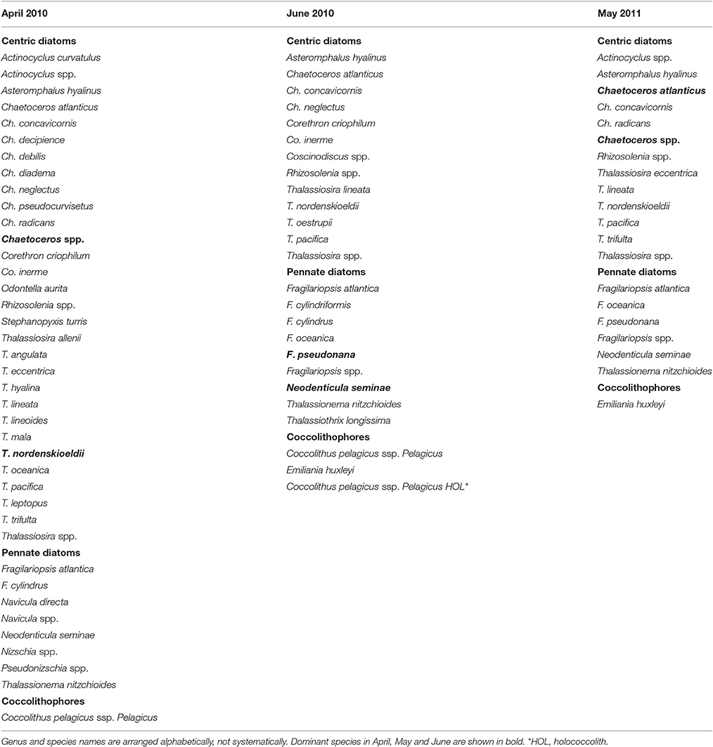
Table 2. List of phytoplankton species identified in Oyashio diatom bloom surveys.
Heterotrophic Bacterial Abundance Estimated by Flow Cytometry
Bacterial abundances in April 2010 and May 2011 were higher in the surface waters than at depth (Figures 2D,F, Table 1). However, in June 2011, little difference was observed from 5 to 300 m (Figure 2E, Table 1). Bacterial abundance within the mixed layer changed only slightly between April 2010 (4.8 ± 0.9 × 10⁵ cells mL−1), June 2010 (3.5 ± 0.9 × 10⁵ cells mL−1), and May 2011 (3.8 ± 1.7 × 10⁵ cells mL−1) (Kruskal-Wallis ANOVA, p = 0.15). Bacteria abundances from 5 to 300 m depths were significantly correlated with those of Chl a concentrations (Spearman's rank correlation, ρ = 0.65, p < 0.001, n = 94). Significant relationships between these were also observed on each cruise (Spearman's rank correlation, April: ρ = 0.75, p < 0.001, n = 16; June: ρ = 0.49, p < 0.005, n = 45; May: ρ = 0.94, p < 0.001, n = 33). Furthermore, there was a significant relationship between bacterial abundance and Chl a within the mixed layer (Spearman's rank correlation, ρ = 0.57, p < 0.01, n = 22). Values of bacteria abundance/Chl a concentration within the mixed layer increased significantly over time, e.g., April 2010 [85 ± 40 cells (pg Chl a)−1], May 2011 [242 ± 68 cells (pg Chl a)−1] and June 2010 [524 ± 70 cells (pg Chl a)−1] (Kruskal-Wallis ANOVA, p < 0.01, Steel-Dwass test, April vs. May: p < 0.01; April vs. June: p < 0.01; May vs. June: p < 0.01).
POC Concentration
The POC concentration at 5-m depth decreased from April through June 2010 (Table 1; April 2010: 454 μg L−1 on average; June 2010: 143 ± 8 μg L−1), and that of May 2011 was 203 ± 37 μg L−1. The ratio of POC/Chl a increased from April through June 2010 (April: 77 on average; June: 237 ± 58), and that in May 2011 was 134 ± 25.
DOC Concentration
DOC concentrations generally decreased from 5 to 300 m depths (Table 1, Figures 2G–I). The highest concentration (~768 μg L−1) was found at 10 and 20 m depths at station J2 and at 10 m at station J3. The lowest concentration (~540 μg L−1) was observed at 300 m depth at stations M2, J3, and J4. The DOC concentration within the mixed layer in June 2010 (744 ± 24 μg L−1) was significantly higher than that in April 2010 (696 ± 12 μg L−1) and May 2011 (708 ± 12 μg L−1) (Kruskal-Wallis ANOVA, p < 0.01, Steel-Dwass test, April vs. May: p = 0.99; April vs. June: p < 0.05; May vs. June: p < 0.01).
POC and DOC Production
POC production at 5 m depth was between 25 mg C m−3 d−1 at the J1 station and 290 mg C m−3 d−1 at the A1 station (Table 1). Average productivity in April and June 2010 and May 2011 decreased from April to June (195 ± 95 mg C m−3 d−1 in April 2010, 72 ± 29 mg C m−3 d−1 in May 2011, and 33 ± 8 mg C m−3 d−1 in June 2010). The average DOC production at 5 m depth in April and June 2010 and May 2011 was 2.9 ± 1.3 mg C m−3 d−1, 1.9 ± 0.5 mg C m−3 d−1, and 3.2 ± 1.0 mg C m−3 d−1, respectively (Table 1). PER ratios were estimated. The average ratios increased slightly from April to June (2.3 ± 1.8% in April 2010, 4.6 ± 0.6% in May 2011, and 5.5 ± 1.5% in June 2010) (Table 1).
TEP Concentration
Minimum and maximum TEP concentrations in our surveys were observed at station A1, at 300 m (<15 μg xanthan gum equiv. L−1) and 20 m (196 ± 71 μg xanthan gum equiv. L−1) respectively (Figures 2K–L, Table 1). TEP concentrations from 5 to 300 m depths were significantly correlated with those of Chl a concentrations throughout the observation period (Spearman's rank correlation, ρ = 0.65, p < 0.001, n = 98) and on each cruise (Spearman's rank correlation, April: ρ = 0.85, p < 0.001, n = 17; June: ρ = 0.52, p < 0.001, n = 47; May: ρ = 0.78, p < 0.001, n = 34). The TEP concentrations were also significantly correlated with bacteria abundance throughout the observation period (Spearman's rank correlation, ρ = 0.65, p < 0.001, n = 98). Additionally, there were significant relationships between the two on each cruise (Spearman's rank correlation, April: ρ = 0.86, p < 0.001, n = 17; June: ρ = 0.36, p < 0.05, n = 48; May: ρ = 0.58, p < 0.001, n = 33).
Average TEP concentrations within the mixed layer in April and June 2010 and May 2011 were 155 ± 12, 90 ± 32, and 112 ± 38 μg xanthan gum equiv. L−1, respectively. TEP levels within the mixed layer in April 2010 were significantly higher than those in June 2010, whereas those in May 2011 were not significantly different from those in April and June 2010 (Kruskal-Wallis ANOVA, p < 0.01, Steel-Dwass test, April 2010 vs. June 2010: p < 0.01, April 2010 vs. May 2011: p = 0.07; May vs. June: p = 0.48). TEP concentrations within the mixed layer in April and June 2010 and May 2011 were also significantly higher than those below the mixed layer in April (64 ± 49 μg xanthan gum equiv. L−1) and June 2010 (67 ± 27 μg xanthan gum equiv. L−1), and May 2011 (81 ± 23 μg xanthan gum equiv. L−1) (Wilcoxon rank-sum test, April: p < 0.01, n = 17; May: p < 0.05, n = 34; June: p < 0.05, n = 48). TEP values were significantly correlated not only with Chl a concentrations but also diatom-derived Chl a biomass (Spearman's rank correlation, TEP vs. Chl a: ρ = 0.70, p < 0.001, n = 23; TEP vs. diatom-derived Chl a: ρ = 0.66, p < 0.001, n = 23). However, no significant relationship was found between TEP levels and Chl a biomass of other phytoplankton groups (Spearman's rank correlation, TEP vs. cryptophytes-Chl a: ρ = −0.22, p = 0.31, n = 23; TEP vs. prasinophyte-derived Chl a: ρ = −0.27, p = 0.22, n = 23; TEP vs. prymnesiophyte-derived Chl a: ρ = −0.28, p = 0.19, n = 23). The TEP/Chl a ratio increased significantly from April to June (26 ± 10 in April 2010, 76 ± 24 in May 2011, and 128 ± 31 in June 2010) (Kruskal-Wallis ANOVA, p < 0.01, Steel-Dwass test, April vs. May: p < 0.01; April vs. June: p < 0.01; May vs. June: p < 0.05). In contrast, values of TEP concentration/bacteria abundance changed little from April and June [0.33 ± 0.06 μg xanthan gum (×106 bacterial cells)−1 in April 2010, 0.34 ± 0.16 μg xanthan gum (×106 bacterial cells)−1 in May 2011, and 0.25 ± 0.07 μg xanthan gum (×106 bacterial cells)−1 in June 2010] (Kruskal-Wallis ANOVA, p < 0.01, Steel-Dwass test, April vs. May: p < 0.01; April vs. June: p < 0.01; May vs. June: p < 0.05).
Laboratory Experiments
Growth Curves, Nutrient Levels, and Chl a Concentrations
Cell abundances in vessels 1 and 2 increased from 2 to ~20,000 cells mL−1 (Figure 4A). As estimated from the specific growth rate, the exponential growth phase was between days 0 and 30 in Vessel 1 and days 0 and 28 in Vessel 2. The stationary phase was observed between days 30 and 40 in Vessel 1 and days 28 and 40 in Vessel 2. The average specific growth rate in both vessels during the exponential growth and stationary phases was 0.31 ± 0.14 d−1 and 0.03 ± 0.07 d−1, respectively (Table 3). The average nitrate, silicate and phosphate levels in both vessels are shown in Figure 4B. During the exponential growth phase, these levels decreased with time. In the stationary phase, nitrate depleted (< 0.1 μM), whereas silicate and phosphate concentrations maintained values of 3.1 ± 0.7 μM and 0.3 ± 0.03 μM. Chlorophyll a concentrations in Vessel 1 (day 20) and 2 (day 18) in the mid-exponential growth phase were 6.1 ± 0.1 μg L−1 and 7.1 ± 0.1 μg L−1, respectively. Ratios calculated from the Chl a concentrations and cell abundance sampled at the same time were 14 pg cell−1 in Vessel 1 and 13 pg cell−1 in Vessel 2 (average 13 ± 1 pg cell−1).
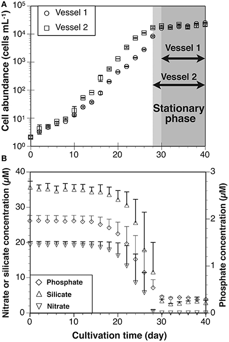
Figure 4. (A) Growth curves of Thalassiosira nordenskioeldii in laboratory cultivation experiment. Each stationary phase in cultivation vessels 1 and 2 is indicated by gray color. (B) Average nitrate, silicate and phosphate concentrations in vessels 1 and 2. Error bars in growth curve and nitrate concentration represent ranges (n = 2).
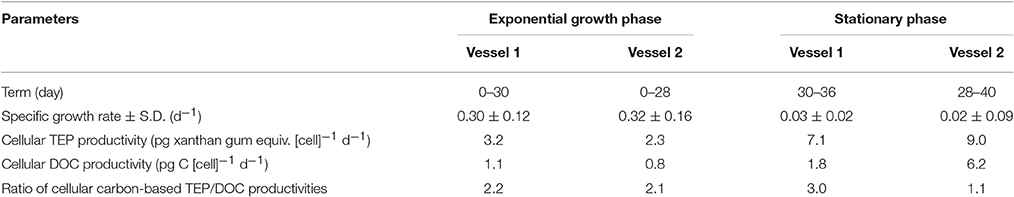
Table 3. Summary of results in exponential growth and stationary phases, obtained from laboratory cultivation experiments.
TEP and DOC Concentrations
The initial (day 0) TEP concentration in Vessel 1 was undetectable, so this concentration was assumed to be 0 μg xanthan gum equiv. L−1. The average TEP concentration in both vessels increased with time (Figure 5). The concentrations ranged from 12 ± 12 μg xanthan gum equiv. L−1 to 1,488 ± 93 μg xanthan gum equiv. L−1. Average DOC concentration also generally increased with time (Figure 5). The concentrations were between 1,148 ± 62 μg C L−1 and 1,647 ± 10 μg C L−1. TEP concentrations in the vessels increased with DOC concentrations (ρ = 0.91, p < 0.001, n = 21).
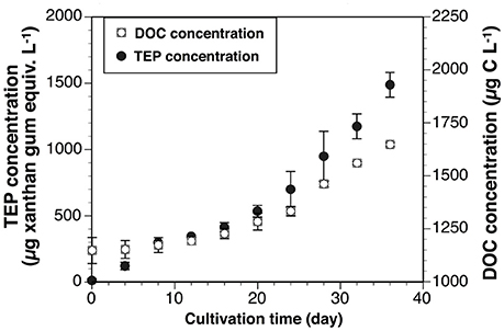
Figure 5. Average TEP and DOC concentrations in vessels 1 and 2 during cultivation experiment.
Cellular TEP and DOC Productivities
Cellular TEP production rates during the exponential and stationary phases were 2.7 ± 0.5 pg xanthan gum equiv. [cell]−1 d−1 and 8.1 ± 0.9 pg xanthan gum equiv. [cell]−1 d−1, respectively (Table 3). Cellular DOC productivity was 1.0 ± 0.2 pg C [cell]−1 d−1 and 4.0 ± 2.2 pg C [cell]−1 d−1 during the exponential and stationary phases, respectively. The cellular TEP and DOC productivities during the exponential growth phase were also converted to a Chl a-normalized TEP production rate (0.21 μg xanthan gum [μg Chl a]−1 d−1) and DOC production rate [0.07 μg C (μg Chl a)−1 d−1], using the factor of Chl a concentration per cell. The cellular TEP and DOC productivities were 2.9 and 4.0-fold greater in the stationary than exponential growth phase, respectively. Ratios of carbon-based TEP/DOC productivities were 2.2 ± 0.02 in the exponential growth phase and 2.0 ± 0.9 in the stationary phase.
Discussion
Factors Controlling TEP Levels in Oyashio Region
According to Kawai (1972), the Oyashio was defined as the water mass where temperatures at 100 m were <5°C. Therefore, all stations in this study were in the Oyashio (Table 1). However, hydrographic conditions were variable throughout the observation period (Table 1). In the Oyashio region, it is known that spring diatom blooms occur during April and May, and decline toward summer every year (e.g., Saito et al., 2002). Indeed, decreases in Chl a concentration were observed from April to June in both 2010 and 2011 as estimated from the satellite images (Supplementary Figure 2).
TEP concentrations from 5 to 300 m depths were significantly correlated with those of Chl a concentrations and with bacteria abundances. Similarly, the TEP concentrations were higher in the mixed layer than in the layer below. These results indicate that TEP was derived from these microorganisms. The Chl a concentrations within the mixed layer decreased significantly from April to June 2010, whereas bacterial cell abundances changed little in that period. The difference in temporal variation between the Chl a concentrations and bacteria abundances within the mixed layer suggest that the main TEP producer was phytoplankton. We used the following Michaelis-Menten-type equation for estimating TEP levels within the surface mixed layer, using Chl a concentration during the spring Oyashio diatom blooms (Figure 6 and Equation 6).
where [TEP]SML is TEP concentration within the surface mixed layer (μg xanthan gum equiv. L−1) and [Chl a] is Chl a concentration within the mixed layer (μg L−1). The root mean square error (RMSE) of this curve was estimated at ± 20 μg xanthan gum equiv. L−1. These findings also suggest that TEP within the surface mixed layer was mainly from phytoplankton.
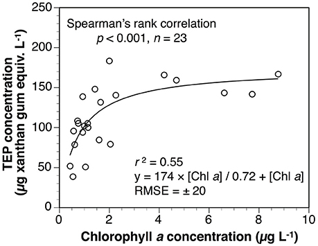
Figure 6. Relationship between TEP and Chl a concentrations within surface mixed layer, revealing significant relationship.
Assuming that TEP was largely produced by phytoplankton, data of each phytoplankton group to Chl a biomass estimated from the CHEMTAX program were useful to discover which group contributed predominately to TEP concentrations. These data showed that diatom-derived Chl a concentrations were dominant in April 2010 (94 ± 4%) and May 2011 (80 ± 9%) (Figure 3). This suggests that the diatoms contributed to the relatively high TEP concentration in our study. In addition, data of phytoplankton species composition by SEM showed that T. nordenskioeldii and Chaetoceros spp. dominated phytoplankton assemblages in April 2010, and C. atlanticus and Chaetoceros spp. were dominant in May 2011 (Table 2). The relatively high TEP levels may have been caused by these diatom species. Compared to April 2010 and May 2011, the dominant phytoplankton groups in June 2010 were diatoms (35 ± 23%), cryptophytes (20 ± 17%), prasinophytes (19 ± 10%), and prymnesiophytes (9 ± 6%) (Figure 3). It has been reported that cryptophytes and prymnesiophytes contribute to high TEP concentrations (Passow et al., 1995; Hong et al., 1997). These phytoplankton groups may have also affected the TEP concentration in June 2010.
Data on TEPs are very limited for the Northwest Pacific. Ramaiah et al. (2005) investigated changes in TEP levels in the Western Subarctic Gyre (WSG) of the North Pacific during an in situ iron fertilization experiment. According to that work, the centric diatom Ch. debilis bloomed in the WSG after iron enrichment, and TEP levels (~50–190 μg xanthan gum equiv. L−1) in an iron-enriched patch increased with Chl a concentration (~1–19 μg L−1) at 5 and 10 m depths. TEP levels found by Ramaiah et al. were similar to those observed in our study. However, Passow (2002a) reported that TEP concentration during diatom blooms can reach > 1,000 μg xanthan gum equiv. L−1 in various regions (Engel, 2000; Prieto et al., 2002). Environmental factors such as temperature, nutrient concentrations, and UV intensity may modulate the TEP production rate of phytoplankton (Mari et al., 2017). An increase of water temperature can raise the TEP production rate (Claquin et al., 2008; Fukao et al., 2012). Seawater temperatures in April 2010 and those in Ramaiah et al. (2005) were relatively low, at 3.1–4.5 and 7.5–9.5°C, respectively. The depletion of nutrients can also increase the TEP concentration because of enhanced release of extracellular polysaccharides (Myklestad, 1995). It has been reported that the ratio of silicate and nitrate concentrations during diatom blooms is relatively constant (approximately 1:1; Brzezinski, 1985; Kudo et al., 2000), and the half-saturation constants of uptake kinetics were ~3 μM in silicate and ~1 μM in nitrate (e.g., Kanda et al., 1985; Nelson and Tréguer, 1992). In April 2010, nutrient concentrations were abundant (> 20 μM in silicate and > 8 μM in nitrate). These results suggest that the lower temperatures and higher nutrients in April 2010 did not increase the TEP levels in seawater much. Recently, Annane et al. (2015) reported lower TEP levels (<200 μg xanthan gum equiv. L−1) during the centric diatom bloom (> 20 μg L−1 in terms of Chl a level, mainly consisting of T. nordenskioeldii) in the lower St. Lawrence Estuary of Canada. The temperature and nitrate concentrations in Annane et al. were similar to those in our study. Therefore, TEP productivity can vary with diatom species and can be relatively low during Oyashio spring diatom blooms when T. nordenskioeldii becomes dominant (Chiba et al., 2004; Suzuki et al., 2011).
Heterotrophic organisms such as eubacteria can also be important in production (e.g., Passow, 2002b; Sugimoto et al., 2007), decomposition (e.g., Passow et al., 2001), and transformation (e.g., Gärdes et al., 2011; Yamada et al., 2013) processes of TEP. Although the present study suggests that the main TEP producer was likely phytoplankton as described above, bacteria abundance was significantly correlated with not only TEP concentration but also Chl a concentration. This indicates close interaction between these microorganisms and TEP. Values of bacteria abundance/Chl a concentration within the mixed layer increased significantly from April 2010 to June 2010, suggesting that relative abundance of bacteria to phytoplankton was low in April 2010. In contrast, TEP levels within the mixed layer were significantly higher in April 2010 than in June 2010. It has been suggested that TEP produced by phytoplankton may serve as protection against hydrolases of attached bacteria (Azam and Smith, 1991; Smith et al., 1995). Hence, the relatively lower Chl a normalized TEP concentrations in April 2010 may have partially contributed to the relative abundance of bacteria to phytoplankton. The lower TEP concentrations may also mean that bacteria had colonized and degraded TEPs. Indeed, the TEPs and their precursors produced by diatoms can be utilized by bacteria. Recently, Cisternas-Novoa et al. (2015) stated that bacterial abundance affected TEP production by T. weissflogii. However, interactions between TEPs and bacteria in nature are complex because of combinations of various environmental factors, as reviewed by Passow (2002b).
Relationship between TEP Production and Phytoplankton Physiology
The TEP levels appeared to decrease from April to June, together with the decline of diatom blooms in the Oyashio region. In contrast, the TEP/Chl a ratio increased significantly from April to June. If the main source of TEP is phytoplankton assemblages, the increase in ratios of TEP/Chl a concentrations from April to June may show that the ability to produce TEP was weaker in diatoms than in other phytoplankton groups, such as cryptophytes, prasinophytes and prymnesiophytes. In our laboratory experimentation, the TEP production rate of the axenic strain of T. nordneskioeldii was estimated at 0.21 μg xanthan gum equiv. [μg Chl a]−1 d−1 during the exponential growth phase. Hong et al. (1997) showed that Chl a-normalized TEP production rates of Phaeocystis antarctica were >500 μg xanthan gum equiv. [μg Chl a]−1 h−1 at photon flux density ~100 μmol photons m−2 s−1. These findings suggest that T. nordenskioeldii was a weaker TEP producer than P. antarctica. In this study, although the sampling from each culture vessel was performed very carefully on a clean bench to avoid any contamination, perhaps bacteria could be slightly contaminated during incubation, and that might underestimate the TEP productivity by T. nordenskioeldii due to its utilization by bacteria. On the other hand, TEP decomposition by bacteria could increase the refractory form of gel particles, because it has been reported that microbial processes can alter the molecular structure of dissolved organic matter (Ogawa et al., 2001). This would contribute to increase in the TEP/Chl a ratio between the bloom and post-bloom phases.
Although diatom species composition possibly affects TEP productivity as mentioned above, the incubation experiment using T. nordenskioeldii revealed that cellular TEP productivity during the stationary phase was 2.9-fold greater than that during the exponential growth phase (Table 3). Changes in physiological state from the exponential to stationary growth phases in this batch culture experiment were likely caused by nitrate depletion (Figure 4B). Therefore, we speculate that nitrate availability probably influences TEP levels during spring diatom blooms in the Oyashio region.
TEP precursors have been considered to be dissolved acid polysaccharides (Thornton et al., 2007; Wurl et al., 2011), which may mainly be from DOC excreted by phytoplankton (Passow, 2002a). Hence, we examined the relationship between TEP levels and DOC production at 5 m depth, but this was not significant (Spearman's rank correlation, p = 0.42, n = 8). In addition, the relationship was evaluated using the axenic strain of T. nordenskioeldii (Chiba et al., 2004; Suzuki et al., 2011). Productivities of cellular TEP and DOC generally varied simultaneously with growth of the diatom strain. These results suggest that TEP production was linked to DOC in the experiment. The in situ DOC production was clearly lower than POC production (Table 1) and was comparable to those (< 0.5–1.2 mg C m−3 d−1) in the Mediterranean Sea between June and July (Lopez-Sandval et al., 2011). However, the PER values were smaller than those (30–41%) in the Mediterranean. In general, relatively low PER values can be found in eutrophic waters (e.g., Hama and Yanagi, 2001; Marañón et al., 2004) and relatively high values were observed in oligotrophic regions (e.g., Alonso-Sáez et al., 2008; Lopez-Sandval et al., 2011). The relatively low PER possibly weaken the relationship between TEP levels and DOC production.
Interestingly, however, the averaged ratio (2.2 ± 0.02) of carbon-based TEP/DOC rates for T. nordenskioeldii in the exponential growth phase was nearly the same as the stationary growth phases (2.0 ± 0.9) (Table 3). If all TEP were formed from DOC released by T. nordenskioeldii, the carbon-based TEP/DOC production ratio would be <1. Our laboratory experiment also found that TEP was rich at the cell surface of T. nordneskioeldii (Supplemental Figure 3). This indicates that some of the DOC excreted by T. nordenskioeldii were trapped on the cell surfaces. Therefore, the carbon-based TEP/DOC production rate > 1 suggests that the TEP was partly formed at cell surfaces. Moreover, the similar carbon-based TEP/DOC production ratios in the exponential and stationary growth phases imply that the formation rate of TEP to DOC was not significantly different between the two phases. The results of our field observations and laboratory experiments imply that high primary production by diatoms leads to relatively strong DOC production, and that subsequently, the excretion of acid polysaccharides (a type of DOC) can generate higher TEP levels in seawater. This was even though the activity of heterotrophic organisms possibly masked the relationship between TEP concentrations and DOC productivity, together with decay of the diatom bloom. Thus, TEP production in the Oyashio region may be enhanced with the increase in DOC production from spring diatoms.
Conclusions
This study revealed TEP dynamics and DOC productivity in the Oyashio region of the Northwest Pacific during spring diatom blooms. Our results showed that TEP levels within the mixed layer were correlated with diatom-derived Chl a biomass, suggesting that diatoms were the main TEP producers. However, TEP levels were not correlated with DOC productivity in the Oyashio region. In contrast, we found that the average TEP and DOC productivities of T. nordenskioedlii varied simultaneously with growth of the strain and that the carbon-based TEP/DOC ratio changed little between the growth phases. These results suggest that TEP productivity in the Oyashio region increases with DOC productivity during spring diatom periods and that TEP removal (e.g., through consumption by heterotrophic organisms) must be considered in evaluating the relationship between TEP levels and DOC productivity. Further laboratory experiments using isolated diatom and bacteria strains should be made to clarify these issues.
Author Contributions
YN and KS designed this research. All authors performed the field observations. The laboratory cultivation experiment was executed by YN. YN analyzed the samples and wrote the paper with KS and YY.
Conflict of Interest Statement
The authors declare that the research was conducted in the absence of any commercial or financial relationships that could be construed as a potential conflict of interest.
Acknowledgments
We thank the captain, crew, and scientists of the FR/V Wakataka-Maru (Tohoku National Fisheries Research Institute, Japan) and R/V Tansei-Maru (JAMSTEC/Atmospheric and Ocean Research Institute, University Tokyo) for their valuable help. We are also grateful to Dr. A. Sugimoto and Ms. Y. Hoshino for 13C analyses of POC and DOC production. Dr. S. Takao is acknowledged for the satellite images. This study was partly supported by the JSPS Grant-in-Aid for Scientific Research (B) (22310002) and Grant-in-Aid for Scientific Research on Innovative Areas (24121004) to KS, and the Sasagawa Scientific Research Grant from the Japan Science Society (24–744) to YN.
Supplementary Material
The Supplementary Material for this article can be found online at: https://www.frontiersin.org/article/10.3389/fmars.2017.00079/full#supplementary-material
References
Alldredge, A. L., Passow, U., and Logan, B. E. (1993). The abundance and significance of a class of large, transparent organic particles in the ocean. Deep Sea Res. I 40, 1131–1140. doi: 10.1016/0967-0637(93)90129-q
Alonso-Sáez, L., Vázquez-Domínguez, E., Cardelús, C., Pinhassi, J., Sala, M., Lekunberri, I., et al. (2008). Factors controlling the year-round variability in carbon flux through bacteria in a costal marine system. J. Geophys. Res. 11, 397–409. doi: 10.1007/s10021-008-9129-0
Annane, S., St-Amand, L., Starr, M., Pelletier, E., and Ferreyra, G. A. (2015). Contribution of transparent exopolymeric particles (TEP) to estuarine particulate organic carbon pool. Mar. Ecol. Prog. Ser. 529, 17–34. doi: 10.3354/meps11294
Ayers, J. M., and Lozier, M. S. (2012). Unraveling dynamical controls on the North Pacific carbon sink. J. Geophys. Res. 117, C01017. doi: 10.1029/2011JC007368
Azam, F., and Smith, D. C. (1991). “Bacterial influence on the variability in the ocean's biochemical state: a mechanistic view,” in Particle Analysis in Oceanography, ed S. Demers (San Diego, CA: NATO ASI Series), 213–236.
Azetsu-Scott, K., and Passow, U. (2004). Ascending marine particles: significance of transparent exopolymer particles (TEP) in the upper ocean. Limnol. Oceanogr. 49, 741–748. doi: 10.4319/lo.2004.49.3.0741
Berman, T., and Viner-Mozzini, Y. (2001). Abundance and characteristics of polysaccharide and proteinaceous particles in Lake Kinneret. Aquat. Microb. Ecol. 24, 255–264. doi: 10.3354/ame024255
Brzezinski, M. A. (1985). The Si:C:N ratio of marine diatoms: interspecific variability and the effect of some environmental variables. J. Phycol. 21, 347–357. doi: 10.1111/j.0022-3646.1985.00347.x
Chiba, S., Ono, T., Tadokoro, K., Midorikawa, T., and Saino, T. (2004). Increased stratification and decreased lower trophic level productivity in the Oyashio region of the North Pacific: a 30-year retrospective study. J. Oceanogr. 60, 149–162. doi: 10.1023/b:joce.0000038324.14054.cf
Cisternas-Novoa, C., Lee, C., and Engel, A. (2015). Transparent exopolymer particles (TEP) and Coomassie stainable particles (CSP): differences between their origin and vertical distributions in the ocean. Mar. Chem. 175, 56–71. doi: 10.1016/j.marchem.2015.03.009
Claquin, P., Probert, I., Lefebvre, S., and Veron, B. (2008). Effects of temperature on photosynthetic parameters and TEP production in eight species of marine microalgae. Aquat. Microb. Ecol. 51, 1–11. doi: 10.3354/ame001187
Engel, A. (2000). The role of transparent exopolymer particles (TEP) in the increase in apparent particle stickiness (α) during the decline of a diatom bloom. J. Plankton Res. 22, 485–497. doi: 10.1093/plank/22.3.485
Engel, A., and Passow, U. (2001). Carbon and nitrogen content of transparent exopolymer particles (TEP) in relation to their Alcian Blue adsorption. Mar. Ecol. Prog. Ser. 219, 1–10. doi: 10.3354/meps219001
Fukao, T., Kimono, K., and Kotani, Y. (2010). Production of transparent exopolymer particles by four diatom species. Fish. Sci. 76, 755–760. doi: 10.1007/s12562-010-0265-z
Fukao, T., Kimoto, K., and Kotani, Y. (2012). Effect of temperature on cell growth and production of transparent exopolymer particles by the diatom Coscinodiscus granii isolated from marine mucilage. J. Appl. Phycol. 24, 181–186. doi: 10.1007/s10811-011-9666-3
Fukuyo, Y., Takano, H., Chihara, M., and Matsuoka, K. (1990). Red Tide Organisms in Japan—An Illustrated Taxonomic Guide. Tokyo: Uchida Rokakuho Publishing.
Gärdes, A., Iversen, M. H., Grossart, H.-P., and Passow, U. (2011). Diatom-associated bacteria are required for aggregation of Thalassiosira weissflogii. ISME J. 5, 436–445. doi: 10.1038/ismej.2010.145
Grossart, H.-P., Berman, T., Simon, M., and Pohlmann, K. (1998). Occurrence and microbial dynamics of macroscopic organic aggregates (lake snow) in Lake Kinneret, Israel, in fall. Aquat. Microb. Ecol. 14, 59–67. doi: 10.3354/ame014059
Grossart, H.-P., Czub, G., and Simon, M. (2006). Algae–bacteria interactions and their effects on aggregation and organic matter flux in the sea. Environ. Microbiol. 8, 1074–1084. doi: 10.111/j.1462-2920.2006.00999.x
Grossart, H.-P., and Simon, M. (1997). Formation of macroscopic organic aggregates (lake snow) in a large lake: the significance of transparent exopolymer particles, phytoplankton, and zooplankton. Limnol. Oceanogr. 42, 1651–1659. doi: 10.4319/lo.1997.42.8.1651
Guillard, R. R. L. (1973). “Division rates,” in Handbook of Phycological Methods: Culture Methods and Growth Measurements, ed J. R. Stein (Cambridge: Cambridge University Press), 289–312.
Guillard, R. R. L. (1975). “Culture of phytoplankton for feeding marine invertebrates” in Culture of Marine Invertebrate Animals, eds W. L. Smith and M. H. Chanley (New York, NY: Plenum Press), 26–60.
Guillard, R. R., and Ryther, J. H. (1962). Studies of marine planktonic diatoms. I. Cyclotella nana Hustedt and Detonula confervacea Cleve. Can. J. Microbiol. 8, 229–239. doi: 10.1139/m62-029
Hama, T., Miyazaki, T., Ogawa, Y., Iwakuma, T., Takahashi, M., Otsuki, A., et al. (1983). Measurement of photosynthetic production of a marine phytoplankton population using a stable 13C isotope. Mar. Biol. 73, 31–36. doi: 10.1007/bf00396282
Hama, T., and Yanagi, K. (2001). Production and neutral aldose composition of dissolved carbohydrates excreted by natural marine phytoplankton populations. Limol. Oceanogr. 46, 1945–1955. doi: 10.4319/lo.2001.46.8.1945
Hattori-Saito, A., Nishioka, J., Ono, T., Michael, R., McKay, L., and Suzuki, K. (2010). Iron deficiency in micro-sized diatoms in the Oyashio region of the western subarctic Pacific during spring. J. Oceanogr. 66, 105–115. doi: 10.1007/s10872-010-0009-9
Honda, M. C. (2003). Biological pump in the northwestern north Pacific. J. Oceanogr. 59, 671–684. doi: 10.1023/b:joce.0000009596.57705.0c
Hong, Y., Smith, W. O. Jr., and White, A.-M. (1997). Studies on transparent exopolymer particles (TEP) production in the Ross Sea (Antarctica) and by Phaeocystis antarctica (prymnesiophyceae). J. Phycol. 33, 368–376. doi: 10.1111/j.0022-3646.1997.00368.x
Ikeda, T., Shiga, N., and Yamaguchi, A. (2008). Structure, biomass, distribution and trophodynamics of the pelagic ecosystem in the Oyashio region, western subarctic Pacific. J. Oceanogr. 64, 339–354. doi: 10.1007/s10872-008-0027-z
Isada, T., Hattori-Saito, A., Saito, H., Ikeda, T., and Suzuki, K. (2010). Primary productivity and its bio-optical modeling in the Oyashio region, NW Pacific during the spring bloom 2007. Deep Sea Res. II 57, 1653–1664. doi: 10.1016/j.dsr2.2010.03.009
Kanda, J., Saino, T., and Hattori, A. (1985). Nitrogen uptake by natural populations of phytoplankton and primary production in the Pacific Ocean: regional variability of uptake capacity. Limnol. Oceanogr. 30, 987–999. doi: 10.4319/lo.1985.30.5.0987
Kasai, H., Saito, H., and Tsuda, A. (1998). Estimation of standing stock of chlorophyll a and primary production from remote-sensed ocean color in the Oyashio region, the western subarctic Pacific, during the spring bloom in 1997. J. Oceanogr. 54, 527–537. doi: 10.1007/bf02742454
Kasai, H., Saito, H., Yoshimori, A., and Taniguchi, S. (1997). Variability in timing and magnitude of spring bloom in the Oyashio region, the western subarctic Pacific off Hokkaido, Japan. Fish. Oceanogr. 6, 118–129. doi: 10.1046/j.1365-2419.1997.00034.x
Kawai, H. (1972). “Hydrography of the Kuroshio and Oyashio,” in Physical Oceanography II: Fundamental Lectures of Oceanography, ed J. Masuzawa (Kanagawa: Tokai University Press), 129–320.
Kudo, I., Yoshimura, T., Yanada, M., and Matsunaga, K. (2000). Exhaustion of nitrate terminates a phytoplankton bloom in Funka Bay, Japan: change in SiO4:NO3 consumption rate during the bloom. Mar. Ecol. Prog. Ser. 193, 45–51. doi: 10.3354/meps193045
Latasa, M. (2007). Improving estimation of phytoplankton class abundance using CHEMTAX. Mar. Ecol. Prog. Ser. 329, 13–21. doi: 10.3354/meps329013
Lopez-Sandval, D. C., Fernández, A., and Marañón, E. (2011). Dissolved and particulate primary production along a longitudinal gradient in the Mediterranean sea. Biogeosciences 8, 815–825. doi: 10.5194/bg-8-815-2011
Mackey, M. D., Mackey, D. J., Higgins, H. W., and Wright, S. W. (1996). CHEMTAX— a program for estimating class abundances from chemical markers: application to HPLC measurements of phytoplankton. Mar. Ecol. Prog. Ser. 144, 265–283. doi: 10.3354/meps144265
Marañón, E., Cermeño, P., and Fernández, E. (2004). Significance and mechanisms of photosynthetic production of dissolved organic carbon in a coastal eutrophic ecosystem. Limnol. Oceanogr. 49, 1652–1666. doi: 10.4319/lo.2004.49.5.1652
Mari, X., and Burd, A. (1998). Seasonal size spectra of transparent exopolymer particles (TEP) in a coastal sea and comparison with those predicted using coagulation theory. Mar. Ecol. Prog. Ser. 163, 63–76. doi: 10.3354/meps163063
Mari, X., Passow, U., Migon, C., Burd, B. A., and Legendre, L. (2017). Transparent exopolymer particles: effects on carbon cycling in the ocean. Prog. Oceanogr. 151, 13–37. doi: 10.1016/j.pocean.2016.11.002
Midorikawa, T., Iwano, S., Kazuhiro, S., Takano, H., Kamiya, H., Ishii, M., et al. (2003). Seasonal changes in oceanic pCO2 in the Oyashio region from winter to spring. J. Oceanogr. 59, 871–882. doi: 10.1023/b.joce.0000009577.40878.d4
Montégut, C. B., Madec, G., Fischer, A. S., Lazar, A., and Indicone, D. (2004). Mixed layer depth over the global ocean: an examination profile data and a profile-based climatology. J. Geophys. Res. 109:C12003. doi: 10.1029/2004jc002378
Myklestad, S. M. (1995). Release of extracellular products by phytoplankton with special emphasis on polysaccharides. Sci. Total Environ. 165, 155–164. doi: 10.1016/0048-9697(95)04549-g
Nelson, D. L., and Tréguer, P. (1992). Role of silicon as a limiting nutrient to Antarctic diatoms: evidence from kinetic studies in the Ross Sea ice-edge zone. Mar. Ecol. Prog. Ser. 80, 255–264.
Ogawa, H., Amagai, Y., Koike, I., Kaiser, K., and Benner, R. (2001). Production of refractory dissolved organic carbon matter by bacteria. Science 292, 917–920. doi: 10.1126/science.1057627
Passow, U. (2002a). Transparent exopolymer particles (TEP) in aquatic environments. Prog. Oceanogr. 55, 287–333. doi: 10.1021/es5041738
Passow, U. (2002b). Production of transparent exopolymer particles (TEP) by phyto- and bacterioplankton. Mar. Ecol. Prog. Ser. 236, 1–12. doi: 10.3354/meps236001
Passow, U., and Alldredge, A. L. (1995). A dye-binding assay for the spectrophotometric measurement of transparent exopolymer particles (TEP). Limnol. Oceanogr. 40, 1326–1335. doi: 10.4319/lo.1995.40.7.1326
Passow, U., Kozlowski, W., and Vernet, M. (1995). Palmer LTER: temporal variability of transparent exopolymer particles in Arthur Harbor during the 1994–1995 growth season. Antarct. J. Rev. 1995, 265–266.
Passow, U., Shipe, R. F., Murray, A., Pak, D. K., Brzezinski, M. A., and Alldredge, A. L. (2001). The origin of transparent exopolymer particles (TEP) and their role in the sedimentation of particulate matter. Cont. Shelf Res. 21, 327–346. doi: 10.1016/S0278-4343(00)00101-1
Prieto, L., Ruiz, J., Echevarría, F., García, C. M., Bartual, A., Gálvez, J. A., et al. (2002). Scales and processes in the aggregation of diatom blooms: high time resolution and wide size range records in a mesocosm study. Deep Sea Res. II 49, 1233–1253. doi: 10.1016/S0967-0637(02)00024-9
Prieto, L., Sommer, F., Stibor, H., and Koeve, W. (2001). Effects of planktonic copepods on transparent exopolymer particles (TEP) abundance and size spectra. J. Plankton Res. 23, 515–525. doi: 10.1098/plank/23.5.515
Radić, T., Kraus, R., Fuks, D., Radić, J., and Pećar, O. (2005). Transparent exopolymer particles distribution in the northern Adriatic and their relation to microphytoplankton biomass composition. Sci. Total Environ. 353, 151–161. doi: 10.1007/s12562-010-0265-z
Ramaiah, N., Takeda, S., Furuya, K., Yoshimura, T., Nishioka, J., Aono, T., et al. (2005). Effect of iron enrichment on the dynamics of transparent particles in the western subarctic Pacific. Prog. Oceanogr. 64, 253–261. doi: 10.1016/j.pocean.2005.02.012
Round, F. E., Crawford, R. M., and Mann, D. G. (2007). The Diatoms Biology & Morphology of the Genera. Cambridge: Cambridge University Press.
Saito, H., Tsuda, A., and Kasai, H. (2002). Nutrient and plankton dynamics in the Oyashio region of the western subarctic Pacific Ocean. Deep Sea Res. II 49, 5463–5486. doi: 10.1016/s0967-0645(02)00204-7
Sakurai, Y. (2007). An overview of the Oyashio ecosystem. Deep Sea Res. II 54, 2526–2542. doi: 10.1016/j.dsr2.2007.02.007
Smith, D. C., Steward, G. F., Long, R. A., and Azam, F. (1995). Bacterial mediation of carbon fluxes during a diatom bloom in a mesocosm. Deep Sea Res. II 42, 75–97. doi: 10.1016/0967-0645(95)00005-B
Sugimoto, K., Fukuda, H., Baki, M. A., and Koike, I. (2007). Bacterial contribution to formation of transparent exopolymer particles (TEP) and seasonal trends in coastal waters of Sagami Bay, Japan. Aquat. Microb. Ecol. 46, 31–41. doi: 10.3354/ame046031
Suzuki, K., Hattori-Saito, A., Sekiguchi, Y., Nishioka, J., Shigemitsu, M., Isada, T., et al. (2014). Spatial variability in iron nutritional status of large diatoms in the Sea of Okhotsk with special reference to the Amur River discharge. Biogeosciences 11, 2503–2517. doi: 10.5194/bg-11-2503-2014
Suzuki, K., Hinuma, A., Saito, H., Kiyosawa, H., Liu, H., Saino, T., et al. (2005). Responses of phytoplankton and heterotrophic bacteria in the northwest subarctic Pacific to in situ iron fertilization as estimated by HPLC pigment analysis and flow cytometry. Prog. Oceanogr. 64, 167–187. doi: 10.1016/pocean.2005.02.007
Suzuki, K., Kuwata, A., Yoshie, N., Shibata, A., Kawanobe, K., and Saito, H. (2011). Population dynamics of phytoplankton, heterotrophic bacteria, and viruses during the spring bloom in the western subarctic Pacific. Deep Sea Res. I 58, 575–589. doi: 10.1016/j.dsr.2011.03003
Suzuki, K., Saito, H., Isada, T., Hattori-Saito, A., Kiyosawa, H., Nishioka, J., et al. (2009). Community structure and photosynthetic physiology of phytoplankton in the northwest subarctic Pacific during an in situ iron fertilization experiment (SEEDS-II). Deep Sea Res. II 56, 2733–2744. doi: 10.1016/j.dsr2.2009.06001
Suzuki, K., Tsuda, A., Kiyosawa, H., Takeda, S., Nishioka, J., Saino, T., et al. (2002). Grazing impact of microzooplankton on a diatom bloom in a mesocosm as estimated by pigment-specific dilution technique. J. Exp. Mar. Biol. Ecol. 271, 99–120. doi: 10.1016/s0022-0981(02)00038-2
Takahashi, T., Sutherland, S. C., Sweeney, C., Poisson, A., Metzl, N., Tilbrook, B., et al. (2002). Global sea-air CO2 flux based on climatological surface ocean pCO2, and seasonal biological and temperature effects. Deep-Sea Res. II 49, 1601–1622. doi: 10.1016/s0967-0645(02)00003-6
Thornton, D. C. O., Fejes, E. M., DiMarco, S. F., and Clancy, K. M. (2007). Measurement of acid polysaccharides in marine and freshwater samples using Alcian blue. Limol. Oceanogr. Methods 5, 73–87. doi: 10.4319/lom.2007.5.73
Tomas, C. R., Syvertsen, E. E., Steidinger, K. A., Tangen, K., Throndsen, J., and Heimdal, B. R. (1997). Identifying Marine Phytoplankton. London: Academic Press.
Van Heukelem, L., and Thomas, C. S. (2001). Computer-assisted high-performance liquid chromatography method development with applications to the isolation and analysis of phytoplankton pigments. J. Chromatogr. A 910, 31–49. doi: 10.1016/s0378-4347(00)00603-4
Wurl, O., Miller, L., and Vagle, S. (2011). Production and fate of transparent exopolymer particles in the ocean. J. Geophys. Res. 116:C00H13. doi: 10.1029/2011jc007342
Yamada, Y., Fukuda, H., Inoue, K., Kogure, K., and Nagata, T. (2013). Effects of attached bacteria on organic aggregate setting velocity in seawater. Aquat. Microb. Ecol. 70, 261–272. doi: 10.3354/ame01658
Keywords: transparent exopolymer particles, primary production, dissolved organic carbon, diatom bloom, Thalassiosira nordenskioeldii, subarctic Pacific
Citation: Nosaka Y, Yamashita Y and Suzuki K (2017) Dynamics and Origin of Transparent Exopolymer Particles in the Oyashio Region of the Western Subarctic Pacific during the Spring Diatom Bloom. Front. Mar. Sci. 4:79. doi: 10.3389/fmars.2017.00079
Received: 05 October 2016; Accepted: 07 March 2017;
Published: 30 March 2017.
Edited by:
Uta Passow, University of California, Santa Barbara, USAReviewed by:
Eva Ortega-Retuerta, Consejo Superior de Investigaciones Científicas, SpainLuca Zoccarato, University of Trieste, Italy
Copyright © 2017 Nosaka, Yamashita and Suzuki. This is an open-access article distributed under the terms of the Creative Commons Attribution License (CC BY). The use, distribution or reproduction in other forums is permitted, provided the original author(s) or licensor are credited and that the original publication in this journal is cited, in accordance with accepted academic practice. No use, distribution or reproduction is permitted which does not comply with these terms.
*Correspondence: Yuichi Nosaka, yuichi.nosaka@gmail.com
†Present Address: Yuichi Nosaka, Research Center for Creative Partnerships, Ishinomaki Senshu University, Ishinomaki, Japan