Individual species and site dynamics are the main drivers of spatial scaling of stability in aquatic communities

1. Introduction

Stability is a widely and diversely applied concept in ecology, which captures the ability of a system to withstand or recover from internal or external perturbations. Given the multitude of anthropogenic pressures in addition to naturally occurring ones, the stability of ecosystem functions has major impacts on human wellbeing as it affects the reliability of ecosystem service provisioning. The quantification of ecological stability, however, is far from trivial. In addition to difficulties arising from the multi-faceted nature of the concept and the associated types of metrics (Donohue et al., 2016), any measure of stability scales with the spatial and temporal extent of the underlying data, which complicates the upscaling of knowledge acquired from small scale experiments to scales relevant to management and conservation (Chase et al., 2018; Viana and Chase, 2019). It is therefore important to understand how stability at larger spatial scales is influenced by the differences in species responses and the heterogeneity in local conditions and community communities.

Hypotheses on how spatial heterogeneity of species distributions can influence changes in ecological processes across scales were already developed more than 30 years ago (Wiens, 1989; Levin, 1992). One hypothesis is that spatial heterogeneity results in scale domains, i.e., portions of the scale spectrum in which an ecological phenomenon behaves consistently regardless of scale. Levin (1992) summarizes terrestrial and aquatic cases of “disturbance-mediated” systems, in which dynamics become more predictable and less variable at larger spatial scales. He argued that there is no correct scale at which to observe variability, but that the scaling relationship is central to allow for comparisons between habitats or organisms. Since then, a growing body of theoretical studies has well established that spatial asynchrony in fluctuations of the ecological property of interest as well as compensatory dynamics due to species-specific characteristics and interactions are the main mechanisms that determine the slope of increases in stability with spatial scale (Loreau et al., 2003; Loreau and de Mazancourt, 2008). However, it has remained largely unknown how species, community or site characteristics drive the patterns found in natural communities and what the relative contributions of compensatory dynamics across space (same species at different locations) or species populations (different species at same location) are.

Compensatory dynamics across spatial scales are determined by the amount of spatial synchrony between different local populations of the same species caused by spatial heterogeneity of environmental conditions (Walter et al., 2017) and the correlation of their fluctuations over time (Lande and Engen, 1999; Liebhold et al., 2004), often described by the so called “Moran effect” (Moran, 1953). In addition, differences in local species compositions and locally distinct species interactions, such as competition, lead to unique patterns of population dynamics across space, which can have both stabilizing (enhanced asynchrony across sites) and destabilizing (enhanced synchrony across sites) effects (Loreau and de Mazancourt, 2008).

Stabilizing effects across ecological scales, i.e., from population to community level, depend on the amount of variability in the fluctuations of local populations and on the degree of synchrony among these species fluctuations (Loreau and de Mazancourt, 2013; Wang et al., 2019). The latter arises from differences in species-specific responses to environmental conditions or disturbances, where a greater variety in responses will lead to stronger compensatory effects and therefore stabilization. Thus, an increase in sampling area is in most cases accompanied by an increase in species diversity, leading to compensatory dynamics due to species-specific responses even when external forcing is synchronous (Wang and Loreau, 2016). Further, the relative abundance or biomass of species are important, i.e., common vs. rare, since changes in the abundance of a dominant species in response to a certain type of disturbance will have larger effects on the community than abundance changes in rare species. This also implies that contrasting community effects can arise depending on perturbation type (Arnoldi et al., 2019).

In order to close the gap between theory and its empirical application, two theoretical frameworks have been developed that describe and disentangle the influence of ecological mechanisms on the scaling of ecological stability using data from natural systems: (1) The invariability-area relationship (IAR; Wang et al., 2017), which describes the relationship of the invariability I (i.e., stability calculated as the squared inverse of the coefficient of variation) of a measured ecological variable and the spatial extent of the study area. The shape of the IAR essentially reflects the amount of spatial synchrony across sites. In the absence of correlation between local communities, invariability increases proportionally to area, resulting in a slope of 1 on a log–log scale. In the case of perfectly correlated dynamics across space, invariability does not change with area due to the lack of compensatory dynamics, and the slope of the IAR is 0. The shape of the IAR therefore allows us to identify different patterns of synchrony decay across space. Wang et al. (2017) proposed two functions of how spatial environmental conditions can affect the shape of the IAR. Exponential synchrony decay occurs when the correlation between two sites only decreases slightly within a certain distance, but quickly decreases to zero once the study area is extended past this so-called characteristic correlation length. The second pattern describes a linear or saturating pattern on the log–log scale, assuming a power law decay of synchrony with increasing distance between sites. (2) The second recently developed approach is a stability-synchrony framework quantifying the relative contribution of spatial and species insurance mechanisms to meta-community stability (Wang et al., 2019). It partitions the variability of an ecological property at the meta-community level (i.e., entire study area) into four measures of variability at two ecological (population, community) and two spatial scales (local, regional; see Figure 1). This approach also allows to quantify the amount of synchrony between the different scales. The relative contributions of compensatory dynamics can thus be attributed to either spatial or ecological increases in scale.

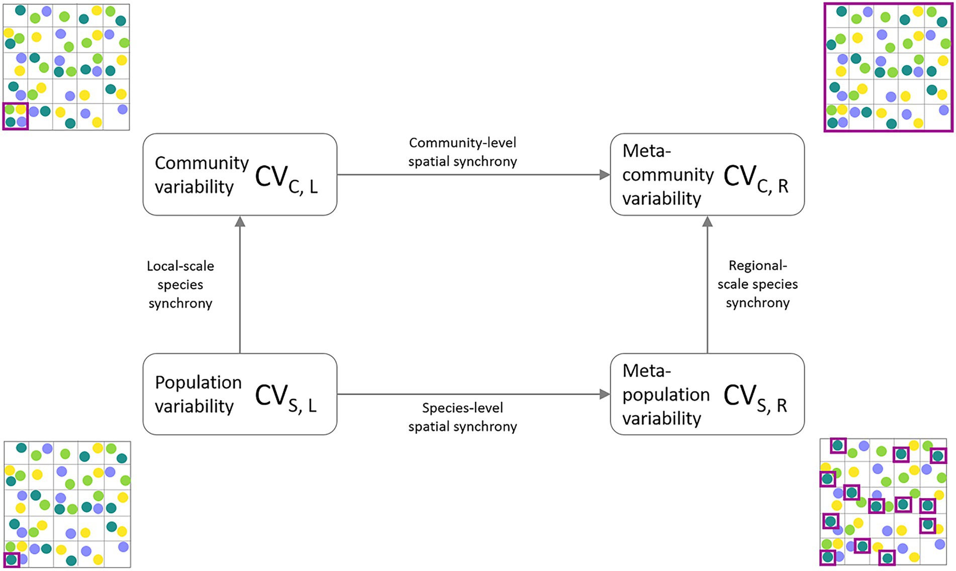
Figure 1. Partitioning framework of meta-community temporal biomass variability (coefficient of variation, CV) into lower levels of spatial scale (local, regional) and ecological organization (species, community). The lowest level of aggregation is represented by average species population variability (CV_S,L, bottom-left corner). The intermediate level of ecological organization is the average community variability (CV_C,L, top-left corner). Spatial aggregation of population variability results in spatially averaged meta-population variability (CV_S,R, bottom-right corner). Meta-community variability (CV_C,R, top-right corner) represents the temporal variability of the total community biomass across the sampling region. The purple squares indicate at which level biomass measurements are aggregated before calculating and averaging the CVs across the entire study region.

In this study, we apply the two frameworks to two freshwater and one marine monitoring data set with time series records on different types of aquatic organisms (freshwater phytoplankton and zooplankton, marine macrozoobenthos). Our aim is to understand the factors governing the relationship between stability and scale in natural aquatic communities and whether its shape can be related to certain system or community properties. In particular, we answer the following questions: (1) How much variability exists in the scaling relationships of stability depending on ecosystem and organism type? (2) Does spatial or ecological scaling contribute more to increasing stability across scales? (3) Do species or sites with high relative biomass values contribute disproportionately to stabilizing or destabilizing effects across spatial scales and are there other community or site characteristics that affect the scaling of stability?

2. Materials and methods

2.1. Data

The first two freshwater data sets originate from a state-wide lake survey program in Iowa, United States (Figure 2), with samplings taking place three times a year in early, mid and late summer (Arbuckle and Downing, 2001). Phytoplankton data were collected using integrated water column samples from the epilimnion (2 m maximum depth) and identified to genus level using light microscopy. Zooplankton samples were collected by vertically towing a Wisconsin net (63 μm mesh) from the thermocline to water surface and identified to the most practical taxonomic level. Biomass values are given in μgL⁻¹ (zooplankton) and mgL⁻¹ (phytoplankton). Filstrup et al. (2014a) and Arbuckle and Downing (2001) provide a comprehensive overview on further methodological details and the study area. The study region covers the entire state of Iowa (146,000 km²). The distance between lake pairs varies between 1 and 484 km. Since missing data points in the biomass time series of the different lakes would have introduced bias when calculating temporal stability of aggregate biomass values, we created a subset of lakes with complete sampling records only. Our subset contains data from 49 lakes (Figure 2) covering all three annual sampling rounds from 2001 to 2007 resulting in 21 data points per time series.

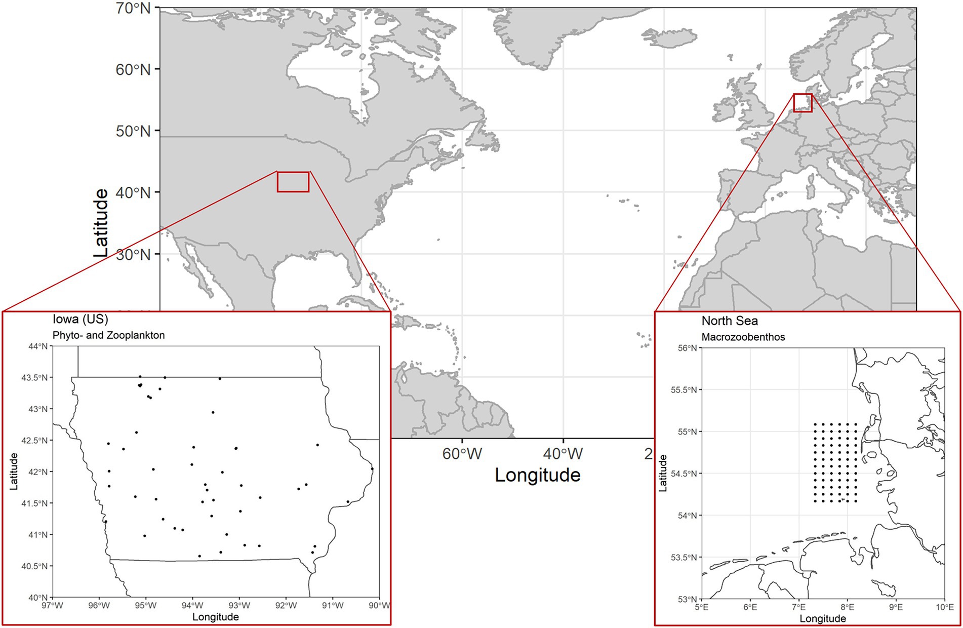
Figure 2. Map containing position of study area and location of single sampling sites for the three monitoring data sets. The sampling locations for phytoplankton and zooplankton samples coincide as they were recorded during sampling occasions of the same sampling campaign. The single sampling locations depict 49 lakes in Iowa (United States). The macrozoobenthos samples were obtained from a monitoring program covering a regular grid of 79 sampling locations off the coast of Northern Germany (North Sea).

The third data set was collected as part of a monitoring program consisting of annual autumn samples on North Sea macrozoobenthos communities off the Northern German coast (Figure 2). Again, we reduced the data set to include only stations with complete sampling records, resulting in a subset of 72 stations over a sampling period of 7 years (2005–2011). Since the original data consisted of abundance records only, we converted it to biomass values (wet weight gm⁻²) using individual biomass estimates from the same species if possible or otherwise the same genus obtained from other North Sea macrozoobenthos sampling campaigns [source: data information systems MARLIN (Federal Maritime and Hydrographic Agency, https://lindevmarlin61.bsh.de/MARLINDMZ/publicSites/MainAppPublic.jsf), CRITTERBASE (Alfred Wegener Institute, https://critterbase.awi.de/)]. Across the 72 stations and 7 years, 195 species were identified. In this data set, sampling sites are arranged across a regular grid with a distance of roughly 10 km between two neighboring stations and a maximum distance of 115 km.

Patterns of local and regional biodiversity and community structure are distinct in each of the monitored species communities. Calculations of Pielou’s evenness index [ranging from complete dominance (0) to complete evenness (1)] revealed on average rather uneven community structures for both phytoplankton (mean = 0.348, std. = 0.053) and macrozoobenthos (mean = 0.399, std. = 0.043) at the local scale. In the phytoplankton data set, the uneven community structure is mainly driven by the strong dominance of the Cyanobacteria genus Microcystis. Similarly, in the North Sea macrozoobenthos data, two dominant species Echinocardium cordatum and Ensis leei in combination with a large number of species with very little and infrequent biomass contributions lead to the low evenness values (Supplementary Figure S1). Dominance patterns in local zooplankton communities were less pronounced (mean = 0.565, std. = 0.024). The average biomass-based Bray–Curtis dissimilarity between pairs of local communities also varied among the phytoplankton (mean = 0.573, std. = 0.064), zooplankton (mean = 0.454, std. = 0.035) and macrozoobenthos (mean = 0.556, std. = 0.041) communities.

2.2. Analysis

We used two approaches to describe the dependence of temporal stability of aggregate community biomass measurements on the spatial extent of the studied area: (1) The invariability-area relationship (IAR, Wang et al., 2017), and (2) a stability-synchrony framework introduced by Wang et al. (2019).

The invariability-area relationship describes the relationship of the invariability I (i.e., stability) of a measured ecological variable and the spatial extent of the study area (A). It is formulated as the inverse of the squared coefficient of variation:

where 𝐴 is the area of aggregation and 𝐶𝑉 is the coefficient of variation of the ecological variable of interest.

In order to investigate how spatial context, i.e., spatial autocorrelation, might affect the slope of the IAR, we apply two different approaches for area increase: (i) the addition of the next closest sampling site for a nested increase of spatial scale and (ii) random addition of sampling sites irrespective of spatial context. We then calculated IARs for all sampling sites. In our study, spatial extent is represented by the number of sampling sites over which the community biomass is aggregated so the increase in spatial extent across the IARs of different stations varies slightly depending on which sampling site was used as starting point.

For the second analysis, we follow the framework introduced by Wang et al. (2019) that allows the distinction between the relative contributions of species vs. spatial insurance effects that increase stability with the level of spatial data aggregation. This partitioning approach results in four measures of variability, represented by the squared coefficient of variation (sensu Wang and Loreau, 2014) at two levels of ecological [species (S), community (C)] as well as spatial [local (L), regional (R) scale (Figure 3)]. These are (1) the variability of local populations (CV_S,L) which is calculated as the weighted average of local population biomass variability across species and sampling locations and stands for the lowest level of spatial as well as ecological aggregation, (2) the variability of local communities (CV_C,L) calculated as the weighted average of community biomass variability across sampling locations, which represents the next higher or intermediate level of ecological aggregation, (3) the meta-population variability (CV_S,R) calculated as the weighted average of the pooled meta-population biomass variability, which serves as a measure for the intermediate level of spatially aggregated variability, and (4) the variability at the meta-community level (CV_C,R) calculated as the weighted overall meta-community variability, i.e., pooled biomass values across all sites and species. For all measures, variability is weighted by the respective overall biomass of a species or community. The up-scaling of variability is possible either by first aggregating biomass values across space and then across levels of ecological organization, i.e., CV_S,L → CV_S,R → CV_C,R, or vice versa, i.e., CV_S,L → CV_C,L → CV_C,R. The variability at the next higher level of data aggregation can be calculated as the product of lower level variability and the synchrony between its components, i.e., at the species (ρ_S) or community level (ρ_C): CV_S,L * ρ_{S → C, L} = CV_{C, L}; CV_S,L * ρ_{S, L → R} = CV_S,R; CV_C,L * ρ_{C, L → R} = CV_C,R; and CV_S,R * ρ_{S → C, R} = CV_C,R.

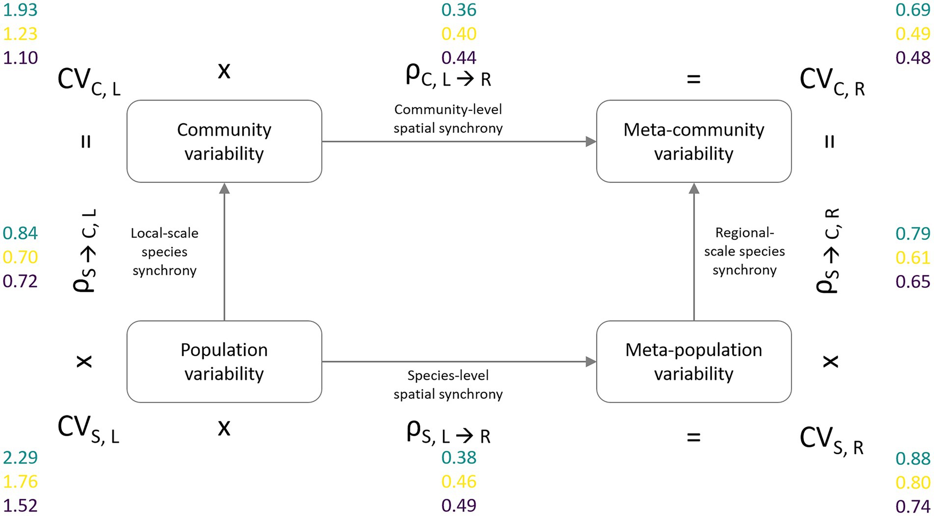
Figure 3. Partitioning framework of meta-community temporal biomass variability (coefficient of variation, CV) into lower levels of spatial scale (local, regional) and ecological organization (species, community). The lowest level of aggregation is represented by average species population variability (CV_S,L, bottom-left corner). The intermediate level of ecological organization is the average community variability (CV_C,L, top-left corner). Spatial aggregation of population variability results in spatially averaged meta-population variability (CV_S,R, bottom-right corner). Meta-community variability (CV_C,R, top-right corner) represents the temporal variability of the total community biomass across the sampling region. The degree of spatial, respectively, species synchrony determines the reduction in temporal variability at the next higher level of spatial and ecological aggregation (e.g., CV_S,L × ρ_{S → C,L} = CV_C,L). Variability and synchrony values are presented for the phytoplankton (green), zooplankton (yellow), and macrozoobenthos (purple) monitoring data sets.

We then generated null model distributions of uncorrelated species population dynamics using cyclic shift permutation (Hallett et al., 2016; Lamy et al., 2019). This approach creates a null model community matrix by assigning random starting points to each individual time series and therefore removing correlations between population dynamics across species and sites while preserving most of the temporal autocorrelation of each individual population. The algorithm has been criticized for not completely preserving autocorrelation structure of species-specific population dynamics (Kalyuzhny, 2020), but for the purpose of comparing between independent population dynamics and dynamics that are driven by ecological mechanisms affecting synchrony patterns across space, these shortcomings are of minor importance.

As sites and species will likely contribute differently to stabilizing or destabilizing mechanisms across space, we ran analyses on all data subsets each time excluding one species (or sampling site), and calculated log response ratios of meta-population and spatial community synchrony to quantify the contribution of each species (or sampling site) to synchrony [i.e., LRR = ln(rho’/rho), sensu Lamy et al., 2019]. We then related the sign and degree of synchrony to site and species-specific characteristics. For sites we used the total, mean and variability of temporal community biomass, effective number of species (ENS), as well as a sites’ compositional uniqueness, represented by its average Bray Curtis dissimilarity from all other sampling locations. As indicators of species characteristics, we calculated a species’ total biomass across sites and sampling occasions, as well as temporal biomass variability, and the heterogeneity of a species’ distribution across the study area, i.e., spatial variability of a species’ biomass.

All statistical analyses were performed using R statistical computing (R Core Team, 2021). The code for the analyses is accessible under https://github.com/DorotheeHodapp/Code-Spatial-Scaling-of-Ecology.

3. Results

3.1. IAR curves

Overall, invariability was lower in the phytoplankton dataset than for the other two organism groups, which was consistent across spatial scales, i.e., local population biomass as well as total metacommunity biomass showed higher temporal fluctuations in the phytoplankton samples (Figure 4). Differences between temporal biomass stability was less pronounced between the species groups at the larger spatial scale indicating a lower degree of stabilization with increasing spatial scale for the zooplankton and macrozoobenthos meta-communities (Figure 4A). For all three species groups, the slope of the IAR was less than one indicating that the observed species dynamics were more synchronous across space than would be expected in case of completely independent biomass fluctuations. The 1:1 line represents the limiting case of completely uncorrelated local species communities whereas a horizontal line indicates complete synchrony across local patches and consequently no increase in invariability with increasing spatial scale. At the local scale, i.e., at a single site, invariability can vary depending on local biomass fluctuations. In our data, both zooplankton and macrozoobenthos communities showed considerably higher invariability than the highly variable phytoplankton communities. This can be caused by either higher synchrony of local species populations or higher overall variability in biomass measurements. The comparison between the two approaches of area increase by aggregating either the next closest sites (Figure 4A) or adding them randomly (Figure 4B) revealed differences in the synchrony decay with increasing level of site aggregation indicating spatially structuring elements in all three data sets.

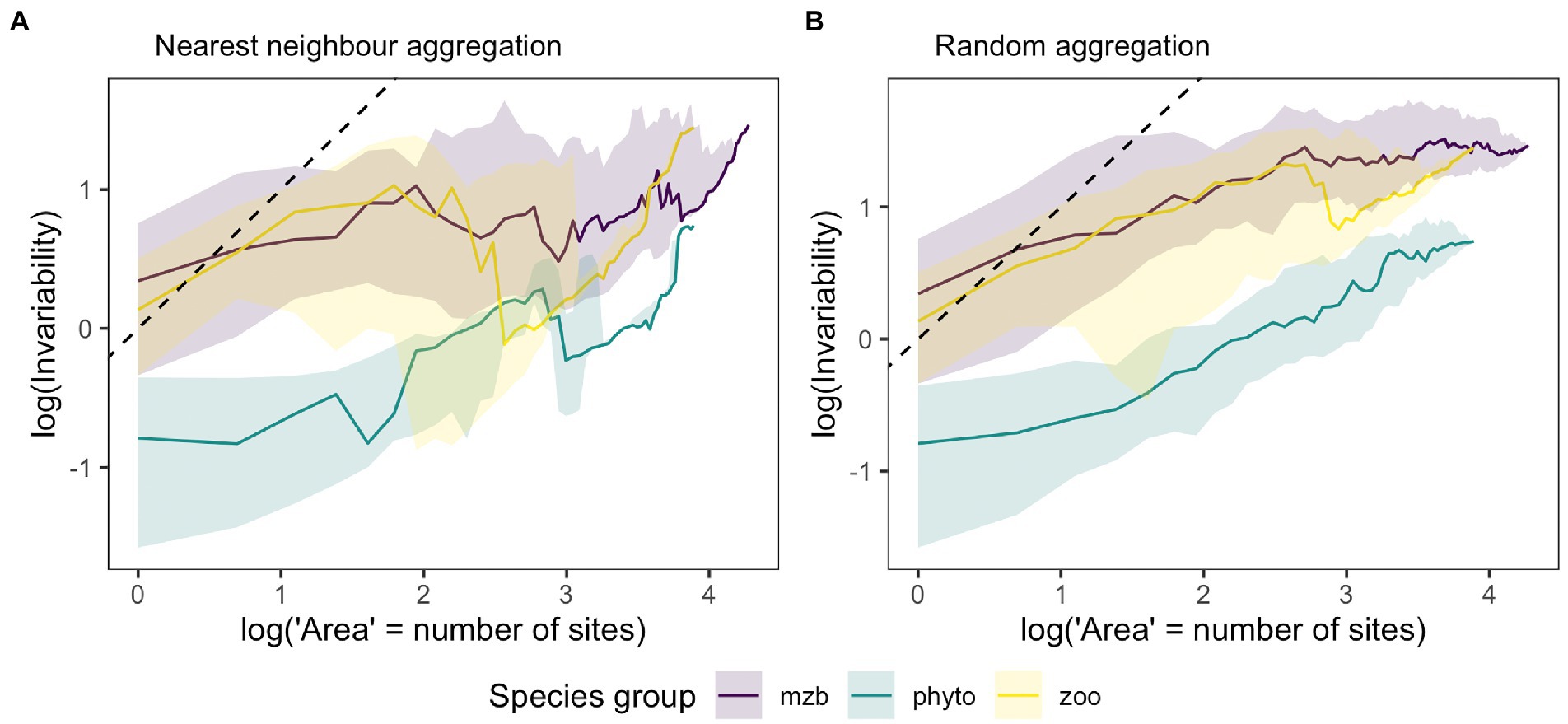
Figure 4. Medians of the invariability-area relationships (IAR) for the phytoplankton (phyto, green), zooplankton (zoo, yellow) and macrozoobenthos (mzb, purple) data sets. Higher invariability, i.e., the inverse of the squared coefficient of variation of aggregated biomass on the y-axis stands for lower temporal biomass fluctuations at a given spatial scale (x-axis), which is represented by the log number of sites that biomass measurements were aggregated over. (A) IARs resulting from spatially nested biomass aggregation, i.e., adding the biomass of the next closest sampling location. (B) IARs generated by randomly drawing a sampling location and adding its biomass for the calculation of invariability at the next higher unit of spatial scale. Shaded areas represent 25 and 75% quantiles. The number of IARs used to calculate the median and quantiles matches the number of sampling locations as each sampling location was used as the starting point for spatial aggregation and IAR calculation once. The black dashed line represents the 1:1 line, which stands for the absence of correlations between local communities.

3.2. Stability-synchrony framework analysis

The second analysis confirmed the IAR results in that temporal variability in local species populations was highest for phytoplankton, followed by zooplankton and macrozoobenthos, which was consistent across all levels of ecological and spatial scale (Figure 3). The reduction in variability when aggregating at the meta-community level was similar for all species groups. Biomass weighted CV² decreased from local species population variability (CV_S,L) to overall meta-community variability (CV_C,R) by a factor of just over three.

Local and regional scale species synchrony yielded synchrony coefficients that were on average twice as large as the spatial synchrony coefficients leading to stronger reductions in variability between spatial levels of aggregation (local ➔ regional) in comparison to the two levels of ecological aggregation (species ➔ community). While the phytoplankton communities showed the highest degrees of species synchrony, they exhibited lower levels in spatial synchrony than the other two species groups. Synchrony measures of zooplankton and macrozoobenthos were similar, although synchrony among zooplankton communities was only slightly but consistently smaller.

The comparison of the synchrony coefficients between the biomass measurements in the three data sets and completely uncorrelated simulated biomass time series yielded higher synchrony levels within and between the natural communities than for the randomly fluctuating population biomasses (Figure 5).

3.3. Stabilizing and destabilizing site- and species-specific characteristics

Overall, absolute values of single species and single site contributions to the stabilization of meta-community biomass follow a clear pattern (Figure 6). A species can have disproportionately high effects on the spatial scaling of stability if it has high total biomass values across space and time or high overall temporal or spatial variability in biomass compared to the other species (Figures 6A–C; Supplementary Table S7). Similarly for sites, high values of temporal mean and variability in biomass can result in greater effects on stabilization or destabilization of temporal biomass values across spatial scales (Figures 6D,E). Importantly, the effects can be positive or negative (Supplementary Figure S6). Sign and magnitude varied in our data depending on species and community characteristics. The effects of community characteristics, i.e., compositional uniqueness, temporal mean and variability of the effective number of species (ENS) on stability patterns across scales differed between the three species groups (Figures 6F–H), most of the relationships were non-significant (Supplementary Table S7). Phytoplankton and macrozoobenthos communities showed higher variability with increasing compositional uniqueness of the community and the mean and temporal variability of species diversity (ENS). For the zooplankton data, there was neither a clear trend in slope nor variation (Supplementary Figures S6F–H).

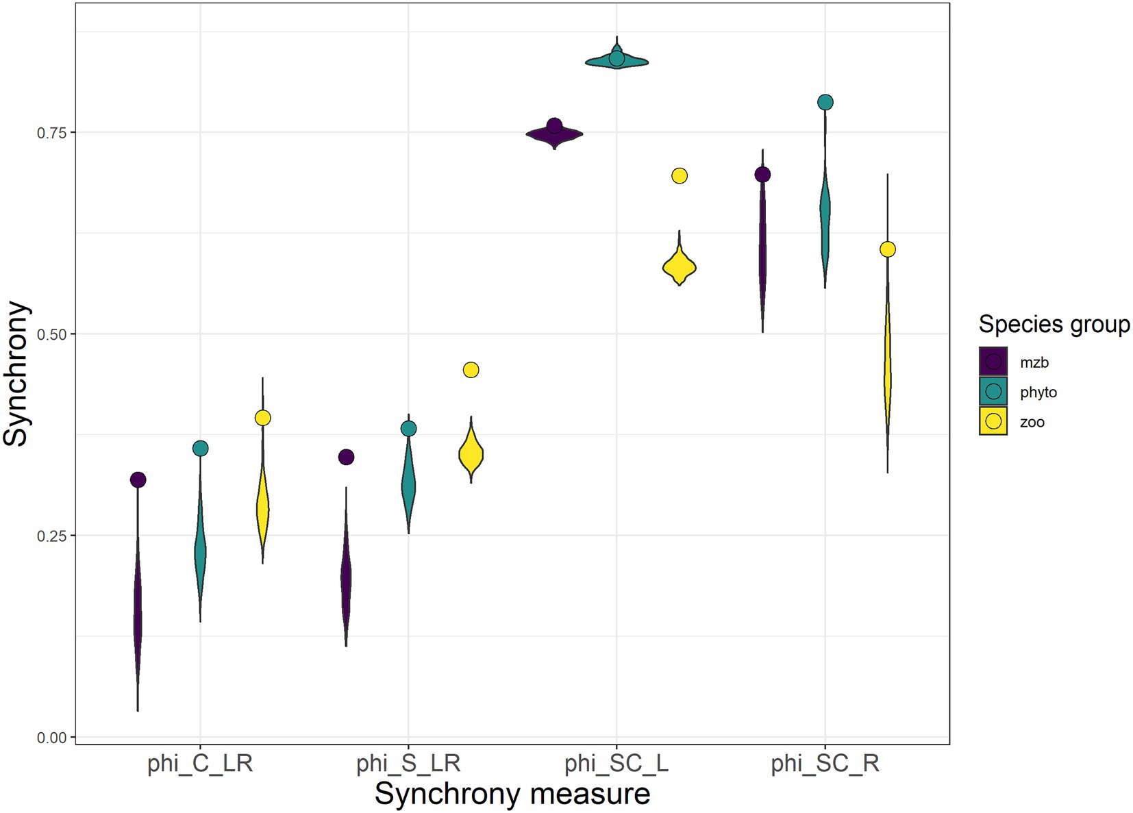
Figure 5. Four metrics of synchrony calculated between the different levels of spatial and ecological scale: the synchrony between local community biomass across space (phi_{C_LR}), the synchrony between populations of one species across space (phi_{S_LR}), the synchrony across species at one site (phi_{SC_L}), and the synchrony between aggregated (regional) species population biomasses (phi_{SC_R}). Violin plots indicate distributions of synchrony coefficients obtained from simulations of uncorrelated population and patch dynamics. The synchrony coefficients calculated from the three monitoring data sets are represented with round symbols. The Colors indicate the three organism types (purple—macrozoobenthos, green—phytoplankton, and yellow—zooplankton).

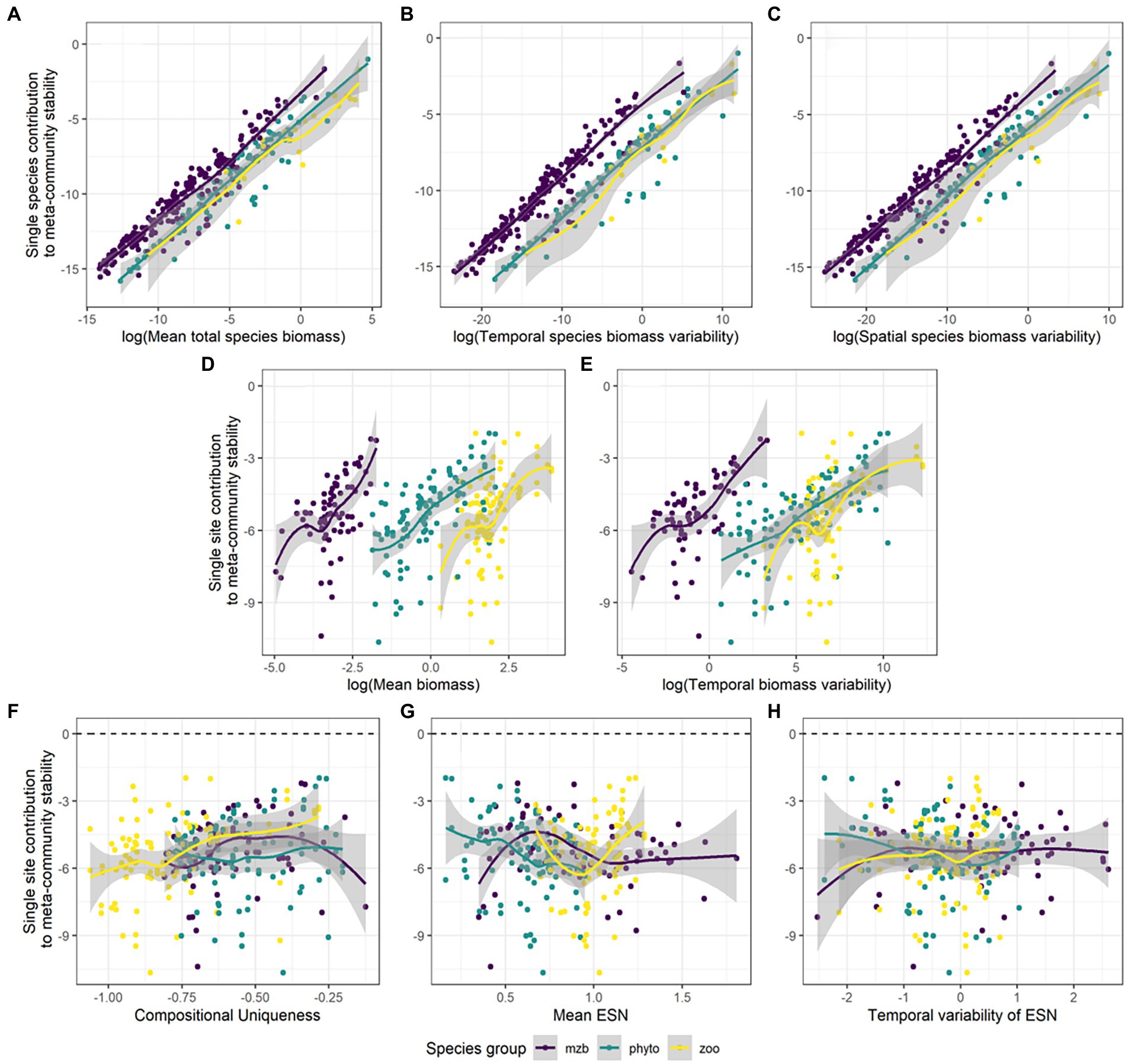
Figure 6. Absolute species and site contributions to the spatial scaling of the temporal stability of meta-community biomass. Species contributions are correlated against their (A) mean total biomasses, (B) temporal biomass variability, and (C) spatial biomass variability. Site contributions are shown in relation to their (D) total biomass, (E) temporal biomass variability, (F) compositional uniqueness, (G) mean effective number of species (ENS) over time, and (H) temporal variability in ENS. The different colors represent the phytoplankton (green), zooplankton (yellow), and macrozoobenthos (purple) monitoring data sets.

4. Discussion

4.1. Shape of the invariability-area relationship

A comparison of IAR shapes across the three organism groups showed on average lower stability levels for phytoplankton communities, i.e., higher temporal variability in biomass than for the two other groups. This difference was consistent at local and regional scales. Potential reasons are the extreme dominance and destabilizing effect of the cyanobacteria Microcystis and the short doubling times of plankton species. In addition, annual bloom formation and succession would likely introduce some synchrony in biomass fluctuations across sampling sites, which could partly be captured by the Iowa lake sampling scheme with samples taken in early, mid and late summer. Zooplankton communities also follow seasonal patterns, but show less pronounced seasonal dynamics as a consequence of longer generation times in comparison to phytoplankton. Their seasonal dynamics are also lower in eutrophic lakes (Sommer et al., 1986) especially if the dominant phytoplankton species are of low edibility or produce toxins like many bloom-forming cyanobacteria species do (Paerl and Otten, 2013). Using the same dataset, Filstrup et al. (2014a) and Heathcote et al. (2016) showed less zooplankton biomass per unit phytoplankton biomass when communities were dominated by few taxa (largely Microcystis). In addition, the lower levels of synchrony in zooplankton and macrozoobenthos communities might be caused by their often patchy distributions in space (Gray, 2002; Armonies and Reise, 2003; Gutow et al., 2020). For the macrozoobenthos data, the yearly sampling scheme and the variable dominance patterns, with different species dominating standing stock biomass across years (Reiss and Kröncke, 2005; Dannheim and Rumohr, 2012; Hodapp et al., 2014), reduced synchrony between sampling locations. For instance, in our data set, the two dominating macrozoobenthos species Echinocardium cordatum and Ensis leei only had peak abundances in a small subset of years over the sampling period and the spatial location of maximum standing stock values also varied considerably between the years (Supplementary Figure S5).

The mean curves of all three species groups (Figure 4A) resemble IAR patterns caused by an exponential synchrony decay, where the correlation between sites abruptly decreases to zero exceeding a certain distance “characteristic correlation length” (Wang et al., 2017). In contrast, our second approach of randomly adding sampling sites irrespective of geographic proximity of single sampling locations yielded IAR curves following a linearly increasing pattern on log–log scale (Figure 4B). This difference concurs with hypotheses on effects of spatially structuring heterogeneity on inter-site synchrony decay across space (Liebhold et al., 2004; Walter et al., 2017). These effects are likely stronger than depicted in our analyses as the necessary averaging across all possible IARs for our set of lakes dilutes effects of individual IAR curves. On the other hand, mean and variability of pairwise correlations across sites are similar for any given distance in the data sets (see Supplementary Figure S3). Reasons for similarities independent of catchment or spatial proximity include the type of land use or location in a watershed. Indeed, there are broad dissimilarities among lakes and watersheds in intensity of the drivers of plankton dynamics (Downing et al., 2008; Filstrup et al., 2016). The macrozoobenthos communities on the other hand are usually associated with specific sediment types introducing local synchrony (Salzwedel et al., 1985; Fiorentino et al., 2017). The patch size of different sediment types can vary greatly thus leading to environmental heterogeneity at much smaller scales than represented by the sampling scheme. One environmental factor likely enhancing synchrony across the whole study area is winter temperature since many macrozoobenthos organisms show lower biomass following cold winters (Neumann et al., 2008). Other common drivers of synchrony across space, such as dispersal (Ranta et al., 2008), community similarity and species interactions, can enhance or even enable the synchronizing effects of the other factors (Vasseur and Fox, 2009). However, these might only play a minor role in our example data sets. Dispersal rates among local populations of macrozoobenthos larval stages are indeed high across space due to recurring exchange of water masses during tidal cycles. However, successful establishment after dispersal driven by differential mortality across species due to physical constraints and biotic interactions (Kröncke and Reiss, 2010; Dannheim and Rumohr, 2012) which combined can lead to low community similarity values.

All three data sets show phases of decreasing stability around intermediate levels of spatial scale. Especially, many of the individual zooplankton and macrozoobenthos IAR relationships show sudden declines in stability after adding specific (highly unstable) sites. It seems that for these two species groups, high variability in biomass more frequently coincides in sites with high biomass values on average and in total (see Supplementary Figure S4) than is the case for the phytoplankton data. This suggests that the correlation between variability and magnitude of biomass across sites (and also species), which can be substantial, likely influences the shape of the IAR curve.

It should be noted that the IARs are affected by a number of study specific factors. As the distance between sites varies, substituting area increase with the addition of a site introduces variability. In addition, as our samples are point estimates, i.e., only represent a fraction of the actual area covered by the respective monitoring scheme, the slope of the IAR might be overestimated as shown in Wang et al. (2017). This is supported by the weak relationship between pairwise temporal correlations of biomass at two sampling locations and their distance (Supplementary Figure S3). Despite these deviations from the model system applied in Wang et al. (2017), the general patterns are consistent across the three data sets and differ from the IARs generated by our second approach of randomly adding sampling sites.

4.2. Stability-synchrony relationships across spatial and organizational levels

For all three data sets, we found stronger stabilizing effects as a consequence of asynchronous biomass fluctuations across space than across species. As previously discussed, seasonal and annual environmental forcing and the sampling scheme likely enhance synchrony across species outweighing much of the temporal variability in biomass dynamics due to species-specific responses. Consequently, depending on the sampling scheme the results could vary as effects of spatial and temporal grain and extent of sampling greatly determine which ecological processes can be detected. In contrast to species-specific fluctuations, local environmental conditions seem to stabilize meta-community biomass by introducing variability in biomass dynamics across space. Drivers of local differences are likely caused by varying land use type (Arbuckle and Downing, 2001) and catchment size which influences nutrient delivery to the lakes (Downing et al., 2008). As a consequence, the lakes and their communities exhibit differing responses to limiting nutrient concentrations. Previous regional studies have also shown that regional characteristics, such as land use, can modify biomass response curves to limiting nutrients (Filstrup et al., 2014a; Filstrup et al., 2014b). In addition, bloom formation depends on several factors other than nutrient availability (Purz et al., 2021) and can therefore be restricted by lake or community specific aspects.

Other examples in the literature found stronger species insurance effects in a kelp forest meta-community, which they explain by niche differentiation among algae species leading to diverse population dynamics due to, e.g., shading tolerance, susceptibility to grazing and wave disturbance (Lamy et al., 2019). In addition, they suspected the high spatial synchrony to be caused by large scale variation in environmental forcing, e.g., sea surface temperature. Another study on spatial scaling of stability in benthic fish communities reported that spatial compensatory dynamics were prevalent in their data and were mainly related to changes in aggregate biomass variability of a certain region (Thorson et al., 2018).

A comparison between spatial and species synchrony in our data sets and simulated meta-communities with randomly fluctuating population biomasses revealed the same or stronger synchrony patterns in the natural communities than expected by chance (also shown in the lower levels of IAR compared to 1:1 line in Figure 4). Given that natural communities at the scale of our study are usually exposed to a set of common environmental drivers, it seems plausible that biomass fluctuations will not be entirely random.

4.3. Effects of species and site characteristics on scaling of stability

Our analyses show that the magnitude and fluctuations of dominant species’ biomass influence which effects single species and sites have on stabilizing processes. Although an addition of sites and species is generally assumed to result in an increase in stability as suggested by the diversity-stability hypothesis, an addition of a highly fluctuating high biomass species can also negatively influence the stability of the aggregated biomass. This is in agreement with the mass-ratio hypothesis (Grime, 1998) stating that community characteristics are usually determined by the traits of the most dominant species. It is also partly inherent in the way stability is measured in both frameworks. In communities with differences in individual biomasses of several magnitudes and highly fluctuating abundances across time and space, species with high total biomass are likely more influential in terms of overall fluctuation of biomass values, i.e., stability. Similar findings have been reported for macroalgal species communities (Lamy et al., 2019) and subtropical forests (Yu et al., 2020), where the influence of the dominant species also outweighed effects of biodiversity on stability. Further, combined effects of single species contributions to stability patterns are not additive, i.e., they cannot be predicted from the single species effects on stability (White et al., 2020). Our research illustrates how dominance is not the sole driver of stability effects. Whether biomass fluctuations of a dominant species result in stabilization or destabilization of community biomass very much depends on the biomass distribution across species and their fluctuations. In our phytoplankton data set, one dominant species is the main driver of community stability across scales with extremely negative effects on community stability. In contrast, the two dominant species in the macrozoobenthos community both stabilized community biomass fluctuations through partly asynchronous dynamics. Consequently, species loss can likewise have stabilizing as well as destabilizing effects on biomass stability and its scaling relationship with space.

In summary, our analysis and comparison of the relationship between ecological stability and increasing spatial extent for three different organism types highlights a few aspects of the spatial scaling of stability in natural species communities. (1) Natural communities are usually more synchronous than expected from completely random dynamics. (2) Despite overall similarities in shape and magnitude of the spatial scaling of stability across data sets of different organisms, our analyses showed that species communities with highly dynamic dominance patterns across space and time foster strong impacts of individual species or locations on stability patterns across space. (3) In addition to single species dynamics, community structure and spatial aggregation of species influence the shape and amount of stability increases with spatial scale. Therefore, our small subset of ecosystem and organism types already highlights a number of variations and potentially associated drivers of scaling of stability across space.

Data availability statement

The original contributions presented in the study are included in the article/Supplementary material, further inquiries can be directed to the corresponding author.

Author contributions

DH and HH conceived the study. WA and JDa provided data for the macrozoobenthos analysis. CF and JDo provided the data for the phytoplankton and zooplankton analyses. DH ran the statistical analyses and wrote the first draft. All authors contributed to the article and approved the submitted version.

Funding

DH and HH acknowledge funding by HIFMB, a collaboration between the Alfred-Wegener-Institute, Helmholtz-Center for Polar and Marine Research, and the Carl-von-Ossietzky University Oldenburg, initially funded by the Ministry for Science and Culture of Lower Saxony (MWK) and the Volkswagen Foundation through the “Niedersächsisches Vorab” grant program (grant number ZN3285). HH was funded by German Science Foundation (DFG HI 848 26-2). JDa acknowledges funding by the Federal Maritime and Hydrographic Agency (grant no.: 10047583).

Acknowledgments

JDo and CF gratefully acknowledge long-term support from the Iowa Department of Natural Resources for the collection of phytoplankton and zooplankton data.

Conflict of interest

The authors declare that the research was conducted in the absence of any commercial or financial relationships that could be construed as a potential conflict of interest.

Publisher’s note

All claims expressed in this article are solely those of the authors and do not necessarily represent those of their affiliated organizations, or those of the publisher, the editors and the reviewers. Any product that may be evaluated in this article, or claim that may be made by its manufacturer, is not guaranteed or endorsed by the publisher.

Supplementary material

The Supplementary material for this article can be found online at: https://www.frontiersin.org/articles/10.3389/fevo.2023.864534/full#supplementary-material

SUPPLEMENTARY DATA SHEET 1 | Iowa Lakes phytoplankton dataset.

SUPPLEMENTARY DATA SHEET 2 | Iowa Lakes zooplankton dataset.

SUPPLEMENTARY DATA SHEET 3 | North Sea macrozoobenthos dataset.

SUPPLEMENTARY DATA SHEET 4 | Supplementary files and figures.

SUPPLEMENTARY DATA SHEET 5 | Metadata for data files.

References

Arbuckle, K. E., and Downing, J. A. (2001). The influence of watershed land use on lake N: P in a predominantly agricultural landscape. Limnol. Oceanogr. 46, 970–975. doi: 10.4319/lo.2001.46.4.0970
Armonies, W., and Reise, K. (2003). Empty habitat in coastal sediments for populations of macrozoobenthos. Helgol. Mar. Res. 56, 279–287. doi: 10.1007/s10152-002-0129-8
Arnoldi, J.-F., Loreau, M., and Haegeman, B. (2019). The inherent multidimensionality of temporal variability: how common and rare species shape stability patterns. Ecol. Lett. 22, 1557–1567. doi: 10.1111/ele.13345
Chase, J. M., McGill, B. J., McGlinn, D. J., May, F., Blowes, S. A., Xiao, X., et al. (2018). Embracing scale-dependence to achieve a deeper understanding of biodiversity and its change across communities. Ecol. Lett. 21, 1737–1751. doi: 10.1111/ele.13151
Dannheim, J., and Rumohr, H. (2012). The fate of an immigrant: Ensis directus in the eastern German bight. Helgol. Mar. Res. 66, 307–317. doi: 10.1007/s10152-011-0271-2
Donohue, I., Hillebrand, H., Montoya, J. M., Petchey, O. L., Pimm, S. L., Fowler, M. S., et al. (2016). Navigating the complexity of ecological stability. Ecol. Lett. 19, 1172–1185. doi: 10.1111/ele.12648
Downing, J. A., Cole, J. J., Middelburg, J. J., Striegl, R. G., Duarte, C. M., Kortelainen, P., et al. (2008). Sediment organic carbon burial in agriculturally eutrophic impoundments over the last century. Global Biogeochem. Cycles 22:GB1018. doi: 10.1029/2006GB002854
Filstrup, C. T., Heathcote, A. J., Kendall, D. L., and Downing, J. A. (2016). Phytoplankton taxonomic compositional shifts across nutrient and light gradients in temperate lakes. Inland Waters 6, 234–249. doi: 10.5268/IW-6.2.939
Filstrup, C. T., Hillebrand, H., Heathcote, A. J., Harpole, W. S., and Downing, J. A. (2014a). Cyanobacteria dominance influences resource use efficiency and community turnover in phytoplankton and zooplankton communities. Ecol. Lett. 17, 464–474. doi: 10.1111/ele.12246
Filstrup, C. T., Wagner, T., Soranno, P. A., Stanley, E. H., Stow, C. A., Webster, K. E., et al. (2014b). Regional variability among nonlinear chlorophyll—phosphorus relationships in lakes. Limnol. Oceanogr. 59, 1691–1703. doi: 10.4319/lo.2014.59.5.1691
Fiorentino, D., Pesch, R., Guenther, C.-P., Gutow, L., Holstein, J., Dannheim, J., et al. (2017). A ‘fuzzy clustering’ approach to conceptual confusion: how to classify natural ecological associations. Mar. Ecol. Prog. Ser. 584, 17–30. doi: 10.3354/meps12354
Gray, J. S. (2002). Species richness of marine soft sediments. Mar. Ecol. Prog. Ser. 244, 285–297. doi: 10.3354/meps244285
Grime, J. P. (1998). Benefits of plant diversity to ecosystems: immediate, filter and founder effects. J. Ecol. 86, 902–910. doi: 10.1046/j.1365-2745.1998.00306.x
Gutow, L., Günther, C.-P., Ebbe, B., Schückel, S., Schuchardt, B., Dannheim, J., et al. (2020). Structure and distribution of a threatened muddy biotope in the South-Eastern North Sea. J. Environ. Manage. 255:109876. doi: 10.1016/j.jenvman.2019.109876
Hallett, L. M., Jones, S. K., MacDonald, A. A. M., Jones, M. B., Flynn, D. F. B., Ripplinger, J., et al. (2016). CODYN:AnR package of community dynamics metrics. Methods Ecol. Evol. 7, 1146–1151. doi: 10.1111/2041-210X.12569
Heathcote, A., Filstrup, C., Kendall, D., and Downing, J. (2016). Biomass pyramids in lake plankton: influence of cyanobacteria size and abundance. Inland Waters 6, 250–257. doi: 10.5268/IW-6.2.941
Hodapp, D., Kraft, D., and Hillebrand, H. (2014). Can monitoring data contribute to the biodiversity-ecosystem function debate? Evaluating data from a highly dynamic ecosystem. Biodivers. Conserv. 23, 405–419. doi: 10.1007/s10531-013-0609-y
Kalyuzhny, M. (2020). Null models for community dynamics: beware of the cyclic shift algorithm. Glob. Ecol. Biogeogr. 29, 1085–1093. doi: 10.1111/geb.13083
Kröncke, I., and Reiss, H. (2010). Influence of macrofauna long-term natural variability on benthic indices used in ecological quality assessment. Mar. Pollut. Bull. 60, 58–68. doi: 10.1016/j.marpolbul.2009.09.001
Lamy, T., Wang, S., Renard, D., Lafferty, K. D., Reed, D. C., and Miller, R. J. (2019). Species insurance trumps spatial insurance in stabilizing biomass of a marine macroalgal metacommunity. Ecology 100:e02719. doi: 10.1002/ecy.2719
Lande, R., and Engen, S. (1999). Spatial scale of population synchrony: environmental correlation versus dispersal and density regulation. Am. Nat. 154, 271–281. doi: 10.1086/303240
Levin, S. A. (1992). The problem of pattern and scale in ecology: the Robert H. MacArthur award lecture. Ecology 73, 1943–1967. doi: 10.2307/1941447
Liebhold, A., Koenig, W. D., and Bjørnstad, O. N. (2004). Spatial synchrony in population dynamics. Annu. Rev. Ecol. Evol. Syst. 35, 467–490. doi: 10.1146/annurev.ecolsys.34.011802.132516
Loreau, M., and de Mazancourt, C. (2008). Species synchrony and its drivers: neutral and nonneutral community dynamics in fluctuating environments. Am. Nat. 172, E48–E66. doi: 10.1086/589746
Loreau, M., and de Mazancourt, C. (2013). Biodiversity and ecosystem stability: a synthesis of underlying mechanisms. Ecol. Lett. 16, 106–115. doi: 10.1111/ele.12073
Loreau, M., Mouquet, N., and Gonzalez, A. (2003). Biodiversity as spatial insurance in heterogeneous landscapes. Proc. Natl. Acad. Sci. 100, 12765–12770. doi: 10.1073/pnas.2235465100
Moran, P. (1953). The statistical analysis of the Canadian lynx cycle. Aust. J. Zool. 1, 291–298. doi: 10.1071/ZO9530291
Neumann, H., Ehrich, S., and Kröncke, I. (2008). Effects of cold winters and climate on the temporal variability of an epibenthic community in the German bight. Climate Res. 37, 241–251. doi: 10.3354/cr00769
Paerl, H. W., and Otten, T. G. (2013). Harmful cyanobacterial blooms: causes, consequences, and controls. Microb. Ecol. 65, 995–1010. doi: 10.1007/s00248-012-0159-y
Purz, A. K., Hodapp, D., and Moorthi, S. D. (2021). Dispersal, location of bloom initiation, and nutrient conditions determine the dominance of the harmful dinoflagellate Alexandrium catenella: a meta-ecosystem study. Limnol. Oceanogr. 66, 3928–3943. doi: 10.1002/lno.11933
R Core Team (2021). R: A language and environment for statistical computing. Vienna, Austria: R Foundation for Statistical Computing.
Ranta, E., Fowler, M. S., and Kaitala, V. (2008). Population synchrony in small-world networks. Proc. R. Soc. B Biol. Sci. 275, 435–442. doi: 10.1098/rspb.2007.1546
Reiss, H., and Kröncke, I. (2005). Seasonal variability of infaunal community structures in three areas of the North Sea under different environmental conditions. Estuar. Coastal Shelf. Sci. 65, 253–274. doi: 10.1016/j.ecss.2005.06.008
Salzwedel, H., Rachor, E., and Gerdes, D. (1985). Benthic macrofauna communities in the German bight. Bremerhaven, Germany: Institut für Meeresforschung in Bremerhaven.
Sommer, U., Gliwicz, Z., Lampert, W., and Duncan, A. (1986). The PEG-model of seasonal succession of planktonic events in fresh waters. Undefined. Available at: https://www.semanticscholar.org/paper/The-PEG-model-of-seasonal-succession-of-planktonic-Sommer-Gliwicz/e1ae666ec6d1af87bf4b69f6ded00a741d4fda4e (Accessed 28 September 2021).
Thorson, J. T., Scheuerell, M. D., Olden, J. D., and Schindler, D. E. (2018). Spatial heterogeneity contributes more to portfolio effects than species variability in bottom-associated marine fishes. Proc. R. Soc. B Biol. Sci. 285:20180915. doi: 10.1098/rspb.2018.0915
Vasseur, D. A., and Fox, J. W. (2009). Phase-locking and environmental fluctuations generate synchrony in a predator–prey community. Nature 460, 1007–1010. doi: 10.1038/nature08208
Viana, D. S., and Chase, J. M. (2019). Spatial scale modulates the inference of metacommunity assembly processes. Ecology 100:e02576. doi: 10.1002/ecy.2576
Walter, J. A., Sheppard, L. W., Anderson, T. L., Kastens, J. H., Bjørnstad, O. N., Liebhold, A. M., et al. (2017). The geography of spatial synchrony. Ecol. Lett. 20, 801–814. doi: 10.1111/ele.12782
Wang, S., Lamy, T., Hallett, L. M., and Loreau, M. (2019). Stability and synchrony across ecological hierarchies in heterogeneous metacommunities: linking theory to data. Ecography 42, 1200–1211. doi: 10.1111/ecog.04290
Wang, S., and Loreau, M. (2014). Ecosystem stability in space: α, β and γ variability. Ecol. Lett. 17, 891–901. doi: 10.1111/ele.12292
Wang, S., and Loreau, M. (2016). Biodiversity and ecosystem stability across scales in metacommunities. Ecol. Lett. 19, 510–518. doi: 10.1111/ele.12582
Wang, S., Loreau, M., Arnoldi, J.-F., Fang, J., Rahman, K. A., Tao, S., et al. (2017). An invariability-area relationship sheds new light on the spatial scaling of ecological stability. Nat. Commun. 8:15211. doi: 10.1038/ncomms15211
White, L., O’Connor, N. E., Yang, Q., Emmerson, M. C., and Donohue, I. (2020). Individual species provide multifaceted contributions to the stability of ecosystems. Nat. Ecol. Evolut. 4, 1594–1601. doi: 10.1038/s41559-020-01315-w
Keywords: ecological stability, spatial scale, ecological scale, synchrony, invariability-area relationship, insurance effect
Citation: Hodapp D, Armonies W, Dannheim J, Downing JA, Filstrup CT and Hillebrand H (2023) Individual species and site dynamics are the main drivers of spatial scaling of stability in aquatic communities. Front. Ecol. Evol. 11:864534. doi: 10.3389/fevo.2023.864534
Edited by:
Paulo AV Borges, University of the Azores, PortugalReviewed by:
Shaopeng Wang, Peking University, ChinaJay E. Diffendorfer, United States Department of the Interior, United States
Pierre Quévreux, UMR5321 Station d'Ecologie Théorique et Expérimentale (SETE), France
Copyright © 2023 Hodapp, Armonies, Dannheim, Downing, Filstrup and Hillebrand. This is an open-access article distributed under the terms of the Creative Commons Attribution License (CC BY). The use, distribution or reproduction in other forums is permitted, provided the original author(s) and the copyright owner(s) are credited and that the original publication in this journal is cited, in accordance with accepted academic practice. No use, distribution or reproduction is permitted which does not comply with these terms.
*Correspondence: Dorothee Hodapp, ✉ dorothee.hodapp@hifmb.de