Drivers and Seasonal Variability of Redox-Sensitive Metal Chemistry in a Shallow Subterranean Estuary
 Alison E. O'Connor
 Elizabeth A. Canuel
 Aaron J. Beck
- 1Virginia Institute of Marine Science, William & Mary, Gloucester Point, VA, United States
- 2Ramboll, Beachwood, OH, United States
- 3GEOMAR, Kiel, Germany
The subterranean estuary (STE) has been historically defined in terms of the mixing of saline and fresh water, in an analogy to surface estuaries. However, redox gradients are also a defining characteristic of the STE and influence its role as a source or sink for metals in the environment. Approaching the STE from a redox-focused biogeochemical perspective (e.g., considering the role of microbial respiration and availability of organic matter) provides the ability to quantify drivers of metal transport across spatial and temporal scales. This study measured the groundwater composition of a shallow STE over 2 years and used multiple linear regression to characterize the influence of salinity and redox chemistry on the behavior of redox-sensitive metals (RSMs) including Mo, U, V, and Cr. Molybdenum and uranium were both supplied to the STE by surface water, but differed in their removal mechanisms and seasonal behavior. Molybdenum showed non-conservative removal by reaction with sulfide in all seasons. Sulfide concentrations at this site were consistently higher than required for quantitative reaction with Mo (10 µM sulfide), evidently leading to quantitative removal at the same depth regardless of season. In contrast, U appeared to depend directly on microbial activity for removal, and showed more extensive removal at shallower depths in summer. Both V and Cr were elevated in meteoric groundwater (2.5–297 nM and 2.6–236 nM, respectively), with higher endmember concentrations in summer. Both V and Cr also showed non-conservative addition within the STE relative to conservative mixing among the observed endmembers. The mobility of V and Cr in the STE, and therefore their supply to the coastal ocean, was controlled by the availability of dissolved organic matter and Fe, suggesting V and Cr were potentially complexed in the colloidal fraction. Complexation by different organic matter pools led to seasonal variations in V but greater interannual variability of Cr. These results reveal distinct behaviors of RSMs in response to seasonal biogeochemical processes that drive microbial activity, organic matter composition, and complexation by inorganic species.
1 Introduction
Submarine groundwater discharge (SGD), advection of water across the seafloor into the coastal ocean, is an important source of nutrients and trace metals to the sea (Spinelli and Fisher 2002; Burnett et al., 2003; Slomp and Van Cappellen 2004; Beck et al., 2009). The chemical composition of SGD is affected by reactions that occur within the subterranean estuary (STE), the mixing zone of fresh and saline water within permeable sediments (Moore 1999; Charette and Sholkovitz 2006; Santos et al., 2009). Recent work has shown that the circulation of water through sandy beaches drives substantial biogeochemical redox reactions (Snyder et al., 2004; Anschutz et al., 2009): the intrusion of oxygenated surface water into the beach face and mixing with outflowing anoxic meteoric groundwater creates a redox interface. Redox reactions within the shallow STE affect the cycling of reduced metabolites (such as Fe(II) and sulfide) as well as redox-active trace metals (Santos et al., 2011; McAllister et al., 2015; O'Connor et al., 2015).
Redox-sensitive metals (RSMs) are characterized by different environmental behavior depending on their redox state. The trace metals Mo, U, V, and Cr form soluble oxyanions under oxidizing conditions, but their reduced species are particle reactive (Bruland and Lohan 2006). Due to their redox-active behavior, these RSMs are widely used as marine paleoproxies to examine oceanic oxygen levels, productivity, and circulation over geologic time scales (e.g., Nameroff et al., 2004; Rimmer et al., 2004; Tribovillard et al., 2006; Algeo et al., 2012). The use of elements like Mo and U as paleoindicators is influenced by material budgets controlling their oceanic concentrations and isotopic composition (Klinkhammer and Palmer 1991; Siebert et al., 2003; Archer and Vance 2008).
The STE may play an important role in controlling RSM budgets in coastal and global oceans; however, the reactions that control RSM concentrations in SGD remain poorly studied. Redox gradients control the porewater concentrations of these elements in both fine-grained sediments (Brumsack and Gieskes 1983; Morford and Emerson 1999; Morford et al., 2005; Scholz et al., 2011), and, although less well studied, in permeable sediments. Uranium removal in the STE has been observed in many locations globally (Duncan and Shaw 2003; Windom and Niencheski 2003; Charette and Sholkovitz 2006; Santos et al., 2011; Riedel et al., 2011). Both non-conservative removal (Windom and Niencheski 2003; Riedel et al., 2011) and addition (Beck et al., 2010) of Mo have been observed in different locations. Although data on V in the STE are limited, both removal and enrichment (Beck et al., 2010; Riedel et al., 2011; Reckhardt et al., 2017) have been observed. Chromium is also poorly studied in the STE, but one study showed non-conservative addition in the mixing zone (O'Connor et al., 2015). In this work, we seek to answer the questions “What biogeochemical processes control RSM distribution in the shallow STE” and “How do these processes change on seasonal and inter-annual time scales”.
Mo, U, V, and Cr have been shown to exhibit distinct behaviors in coastal ocean porewaters (Brumsack and Gieskes 1983; Morford et al., 2005; Scholz et al., 2011) as well as within shallow STEs (O'Connor et al., 2015). These elements differ in the redox potential (Eh) at which they are oxidized/reduced and in their responses to geochemical variables such as sorption to reactive metal oxides, complexation with organic matter or sulfide, and the activity of certain microbial species (Rai et al., 1989; Wanty and Goldhaber 1992; Barnes and Cochran 1993; Lovley et al., 1993; Helz et al., 1996). Therefore, seasonal variation in environmental conditions within the STE suggests that RSMs are likely to exhibit seasonally variable behavior within this zone as well. Redox-sensitivity may lead to environmental modulation of the SGD-driven RSM source to the ocean and may therefore represent an unexplored mechanism of variation over time.
2 Methods
2.1 Study Site
The study site is located on the York River Estuary (YRE) in Gloucester Point, Virginia, United States (37.248884 °N–76.505324 °E) (Supplementary Figure S1A). The YRE is a microtidal (0.7–0.85 m tidal range), relatively uncontaminated tributary of the Chesapeake Bay (Moore and Reay 2009). Salinities of YRE surface water overlying the sediments at this study site typically range from 14 in the winter to 25 in the summer (Luek and Beck 2014). The Gloucester Point beach is a narrow (20–30 m wide) sandy beach with a gradual slope (0.2). It is bordered to the east by an upland marsh. Granite breakwaters line the beach ∼40 m from the dune line to prevent erosion and stabilize the beach morphology (Supplementary Figure S1B). Sediment porosity at the study site ranges from 0.26 to 0.41 (O’Connor et al., 2018).
Previous work at the study site used a Ra budget to estimate seasonally variable SGD volume fluxes to the York River between 93 and 178 L m−2 d−1 (Luek and Beck 2014), comparable to other SGD fluxes estimated using Ra (Cable et al., 1996; Burnett et al., 2008). Groundwater hydraulic head at the study site is inversely correlated with tidal height (Beck et al., 2016), and seasonal fluctuations in groundwater and sea level control saline water intrusion and groundwater discharge (Luek and Beck 2014). Previous sampling of redox-active constituents at the same mid-tide location showed that advection of water through the sandy sediments drives the formation of a “classic” redox sequence typical of diffusion-dominated fine-grained sediments (O'Connor et al., 2015). Sediments at the mid-tide line (MT; Supplementary Figure S1C) are oxic down to ∼70 cm depth, exhibit a peak in NOx between 70 and 100 cm, followed by a peak in dissolved Fe and Mn starting at 100 cm, and increasing sulfide below approximately 140 cm depth (depths relative to the high tide sediment surface level) (O'Connor et al., 2015). The vertical distributions of DOC and reduced metabolites remained consistent over time, but concentrations varied with season (O'Connor et al., 2018). Dissolved organic carbon concentrations were greatest in the summer, and shallow meteoric groundwater supplied the majority of DOC to the STE. Dissolved Fe and Mn were highest in a plume through the middle of the STE (100–140 cm) that was characterized by both higher concentrations and greater non-conservative addition in the winter. In contrast, sulfide was higher in summer at depths within the Fe and Mn plume (100–140 cm). The general distributions of RSMs have also been previously described (O'Connor et al., 2015). Both Mo and U were supplied to the STE from overlying estuarine water, and V and Cr had a mid-depth maximum at a sampling profile bisecting the shallow STE (O'Connor et al., 2015).
2.2 Groundwater Collection and Analysis
Sample collection and analyses have been described previously (O'Connor et al., 2018), and will be discussed briefly here. Groundwater samples were collected using permanently installed wells comprising a 1 cm-long stainless steel screened point (AMS, Inc.; e.g., Gonneea et al., 2013) attached to 3 mm diameter No-Ox® PTFE tubing (Supelco/Sigma-Aldrich), or from an all-plastic multi-level sampler (Beck et al., 2007). Low-flow sampling methods were used to minimize oxygen introduction into the sample. Groundwater was pumped from depth using a portable peristaltic pump and filtered through an in-line 0.45 μm Millipore polypropylene capsule filter into sampling containers. Salinity, temperature, and Eh were measured in an included flow-through unit at the time of collection with a hand-held YSI556 multi-probe.
Samples were collected from the mid-tide (MT) profile, located at the center of the shallow saline recirculation cell (Supplementary Figure S1C), each month (March 2013 to February 2015) during the week of spring tide at the ebb phase of the tidal cycle. Groundwater samples were also collected from a shore-normal transect (Figure 1) during 4 months (April 2014, July 2014, October 2014, and February 2015) to capture variations over a year. Depth profiles were collected along a shore-normal transect, at the locations of average water levels during high tide (HT), MT, and low tide (LT). Additional shallow groundwater samples were collected between the HT and MT locations (Figure 1) using a drive-point piezometer to better delineate chemical distributions. To remain consistent between profiles, all depths were calculated relative the sediment surface at the high tide profile (rather than sediment surface at the location of collection).
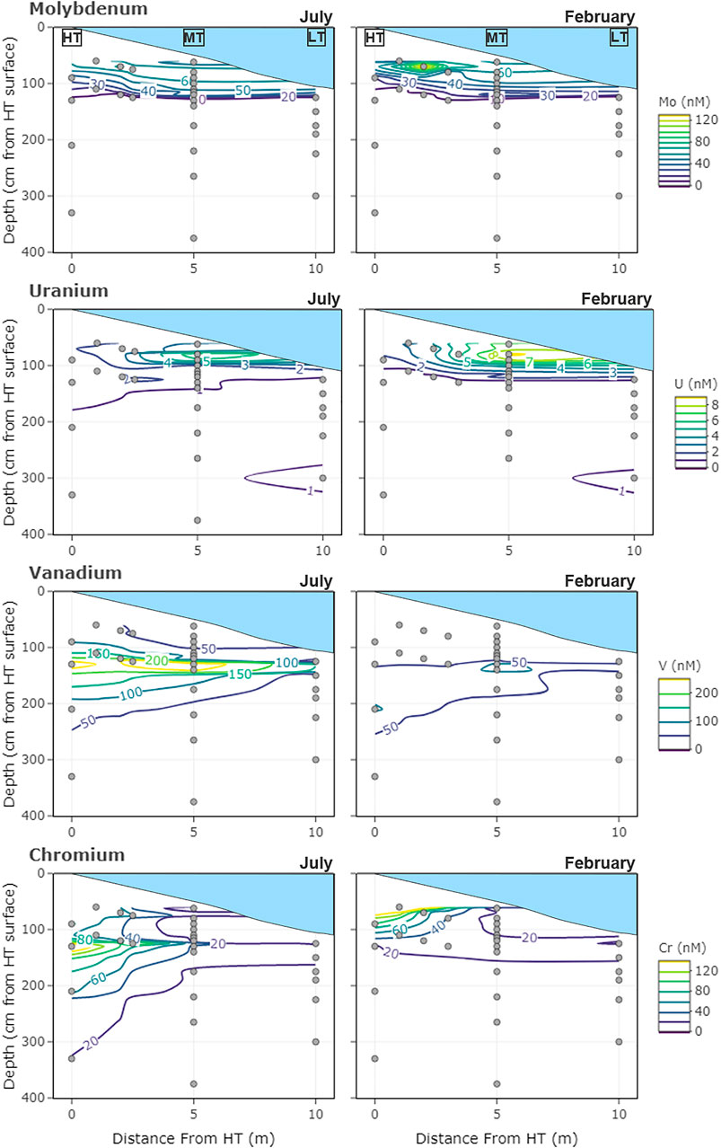
FIGURE 1. Sampling locations of the subterranean estuary transect and concentrations of dissolved redox-sensitive metals (A) Mo (B) U (C) V, and (D) Cr measured in July 2014 and February 2015. Depth profiles were located at the spring high tide (HT), mid-tide (MT), and just below low tide (LT) water levels. Depths are measured relative to the high tide sediment surface (0 cm).
Groundwater samples for dissolved (<0.45 µm) trace metal analysis (Fe, Mn, Mo, U, V, and Cr) were collected in acid-washed LDPE bottles, acidified immediately after collection, and analyzed by two-fold dilution and direct injection on a Thermo Element 2 inductively-coupled plasma mass spectrometer at the University of Southern Mississippi’s Center for Trace Analysis. Isotope dilution was used to account for matrix effects. Detection limits were ≤2 nM (nM). Samples for organic-metal complex measurements (<0.45 µm) were collected during the February seasonal transect sampling in 1 L acid-washed LDPE bottles and immediately frozen. These samples were later thawed and extracted through a Bond Elut C18 column (Agilent, 500 mg bed mass). Columns were acid-washed in dilute trace metal grade HCl and rinsed thoroughly. Before use, columns were conditioned with 100 ml of methanol followed by 500 ml of MilliQ water. Approximately 250 ml of sample was loaded through the column (confirmed by sample mass difference), followed by a 10 ml MilliQ water rinse (Lemaire et al., 2006). The column was dried by pulling air through for 30 minutes, and then elution was done with 10 ml of HPLC-grade methanol. Concentrated ultrapure HNO3 (100 µL) was added to samples before they were dried under a HEPA-filtered laminar flow hood. Samples were reconstituted with 1 N ultrapure HNO3 for analysis as described above. This method isolates 20–60% of DOC, primarily hydrophobic species (Lemaire et al., 2006). The amount of DOC recovered in the extractions here is not reported because efforts to prevent metal contamination were prioritized over preventing organic carbon contamination (e.g., collecting eluent in LDPE bottles). The metals extracted along with this organic phase will be referred to here as associated with hydrophobic dissolved organic matter (hDOM). Due to the uncertainty in DOC recovery in hDOM, the association of metals with hDOM can be considered to be a semi-quantitative assessment of how the metals are associated with DOM overall within the STE; comparisons can be made across space, time, and different metals within the study, but caution should be used if comparing precise numbers to other studies. Details for collection and analysis of DOC, humic C, and sulfide can be found in O’Connor et al. (2018).
2.3 Sediment Collection and Analyses
A 4-m long vibracore was collected adjacent to the mid-tide sampling location in May 2013, and processed as described previously (O'Connor et al., 2018). The core was sectioned into 5 cm intervals to evaluate vertical variations in sediment contents. Sequential leaches were performed to isolate the metal oxide and recalcitrant metal fractions (Tessier et al., 1979). Dried and weighed sediments (∼1 g) were shaken for 180 min in 5 ml of 1 M hydroxylamine hydrochloride in 25% acetic acid, centrifuged at 3000 g for 10 min. Four milliliters of supernatant were removed to a new, clean tube and diluted in 0.5 M HNO3 (Aristar Plus, trace metal grade). This represented the fraction liberated upon reductive dissolution of Fe and Mn (hydr)oxides (Tessier et al., 1979), and will be referred to here as the “metal oxide fraction.” The leach method used in the current study does not provide the specific information about speciation or redox state of solid-phase metal oxides afforded by other chemical leach methods (e.g., Anschutz et al., 2005; Hyacinthe et al., 2006). The simpler leach method was used here to liberate metals associated with the bulk amorphous oxide pool, comparable to other studies of Fe and Mn cycling in the STE (e.g., Charette et al., 2005). The remaining sediment was shaken in 5 ml aqua regia (1:3 HNO3:HCl) for 13 h. Samples were centrifuged, and the supernatant removed and diluted with MilliQ water. Metal concentrations in these fractions were analyzed as described for groundwater samples above. This fraction represents more recalcitrant sedimentary phases (but does not dissolve pyrite) and will be referred to as the “recalcitrant fraction” (Tessier et al., 1979; Huerta-Diaz and Morse 1992). Metal concentrations in both fractions were analyzed as described for groundwater samples above.
2.4 Data Analysis
As previously described (O'Connor et al., 2018), this STE is characterized by three endmember mixing between saline, estuarine surface water and two distinct up-gradient freshwater sources: one shallow and one deep (Supplementary Figure S1C). The shallow freshwater endmember is more oxidizing than the deep endmember (Eh around 100 mV compared to < −100 mV) and has higher organic matter contents. Therefore, mixing of chemical elements could not be evaluated only with respect to a single fresh endmember. To evaluate chemical addition or removal along the seasonal STE transects, two mixing lines were inferred on salinity-concentration plots: one between the surface endmember and the shallow fresh endmember, and one between the surface and deep fresh endmember. Points that fall within the triangle created by the two mixing lines were interpreted as resulting from mixing between the three endmembers, while those falling outside result from non-conservative addition or removal.
To quantify the addition or removal of an element at the MT profile over the 2-years time series, we calculated the concentration anomaly relative to conservative mixing. The concentration anomaly is the difference between the measured concentration and the expected concentration given conservative mixing between the endmembers, calculated as:
The expected concentration (Cexpected) was calculated using the fractional contributions of the three endmembers. The contribution of each endmember was calculated using salinity and humic carbon as tracers (described in O'Connor et al., 2018).
Multiple linear regression models were used to evaluate the response of the RSEs (Mo, U, V, and Cr) to changes in biogeochemically relevant predictor variables. All analyses were performed using existing functions in R (R Core Team 2015). The goal of these regressions was to determine the effect of major groundwater constituents on the distribution of RSMs, providing insight into how these elements respond to geochemical changes in the STE. These relationships also suggest what major constituents could be used to predict RSM behavior in other coastal groundwaters.
Two sets of regressions were used to understand the responses of redox-sensitive trace metals to other chemical constituents in the STE across time and space. The first used data measured monthly at the MT location and explored seasonal changes over the 2 years of sample collection (referred to here as “time effects”). Time effects regressions were performed on MT profile data separated into summer (May to October) and winter (November to April) of 2013 and 2014 (seasons were differentiated by differences in groundwater temperature; O’Connor et al., 2018). The second set of regressions assessed how RSM responses to predictor variables differed along a shore-normal transect (referred to here as ‘space effects’). The space effect regressions were done on the HT, MT, and LT profile data separately (using all 4 months of data at each location) to determine if RSM response to predictor variables differed spatially throughout the STE. Depth ranges included for each well were selected to exclude depths at which a given RSM concentration was consistently below the detection limit (below which any correlation analysis becomes meaningless).
Models using different combinations of geochemically relevant predictor variables were considered. Final models were selected based on p values the Akaike information criterion (AIC). AIC is used to compare the relative quality of potential models, with a lower AIC indicating a higher quality model. The model’s p value indicates the chance that the data fit to a model is due to random chance, rather than due to a true relationship in the data. Therefore, a lower p value indicates that a model is statistically significant. Due to the need to select a model that was the best overall fit for several conditions, a hard cut-off for p value was not used. Rather, a combination AIC and p value were evaluated in combination. In reporting model results, all R2 values reported are the adjusted R2 of the model which accounts for the sample size.
All response variables (i.e., RSM concentrations), as well as salinity, dissolved Fe, DOC, humic C, and sulfide concentrations were natural log transformed to achieve data normality. Temperature data were normal without transformation. In cases where DOC and humic C were both predictors in a model, collinearity was checked using the variance inflation factor (VIF). The VIF never exceeded 5, the recommended cut-off for multicollinearity in a model (James et al., 2014), so both predictors were retained in these cases.
The biogeochemical rationales for inclusion of various predictor variables considered for inclusion are described here. Salinity was considered for inclusion in all models to account for mixing of fresh and saline waters. Temperature was considered for the space effect models because chemical reactions (both biotic and abiotic) are temperature dependent. The time effects model, already split up by season, accounted for temperature in its design and temperature was therefore not considered as a possible predictor.
Dissolved Fe was considered as a predictor in all Mo and U models because Mo(VI) can sorb to iron oxides, and some Fe reducing bacteria can reduce U. Sulfide was considered in all Mo and U models because sulfide reacts directly with Mo, and because several sulfur-reducing microbial species are capable of reducing U. Although U(VI) can be reduced by Fe(II) (Behrends and Van Cappellen 2005) and sulfide (Hua et al., 2006), the rates of these reactions are comparable to those of enzymatic reduction only under certain conditions (e.g., the ready availability of certain reactive metal hydroxide surfaces; dominance of uranium hydroxide species). Therefore, geochemical associations of U with Fe and S here are generally considered to be proxy relationships for the microbial processes that generate these reduced metabolites, although abiotic reduction may also play a role.
DOC, humic C, and dissolved Fe were considered for all V and Cr models because reduced V and Cr species can be complexed by organic matter (Wehrli and Stumm 1989; Remoundaki et al., 2007) and co-precipitate with iron (hydr)oxides (Rai et al., 1989).
Model results are presented using normalized coefficient plots. For a given model, the coefficients are calculated based on scaled and centered data (using the scale function in R) in order to be comparable across different predictors. Stronger relationships between predictor and response variables are represented by larger (either positive or negative) coefficients. Normalized coefficients and p values can be found in the Supplementary Material.
3 Results
3.1 Groundwater
3.1.1 Molybdenum
The mean concentration of Mo in the shallow freshwater endmember (7.8 ± 4 nM) tended to be higher than for the mean deep freshwater endmember (0.63 ± 1 nM), but both were much lower than estuarine surface water concentrations (63 ± 8 nM) (Table 1). Molybdenum was highest in the surface water and shallow STE groundwater, with the 25 nM contour falling between 50 and 150 cm depth, and the 10 nM contour between 100 and 200 cm depth (Figure 1A). At MT, concentrations decreased steadily from surface water concentrations (62 ± 11 nM in summer; 57 ± 9 nM in winter) to 24 ± 12 nM at 115 cm depth across all seasons (Figure 2A). Below 115 cm depth, Mo declined sharply to less than the detection limit of 1 nM. At LT, Mo was consistently lower than at other locations (3 ± 5 nM) but tended to be highest in the shallowest sampled depth (Figure 1A). Concentrations of dissolved Mo associated with hDOM were highest at depths between 50 and 100 cm throughout the STE, reaching 4.5–10.8 nM (Figure 3A). The percent of Mo associated with hDOM increased with depth in the STE, from 2.7% in the surface to >50% below 150 cm depth (Figure 3A).
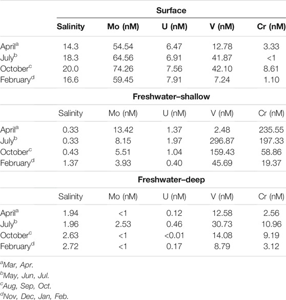
TABLE 1. Endmember salinities and RSM concentrations used to estimate mixing and concentration anomalies. The notes identify the months corresponding to the endmember concentrations that were used to calculate the conservative mixing lines and concentrations.
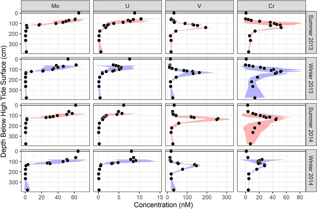
FIGURE 2. Dissolved (A) Mo, (B) U, (C) V, and (D) Cr concentrations from the MT profile over the 2-year time series. Summer is defined as May to October, and winter is defined as November to April. At each depth, the filled circles represent the mean, and shaded areas represent one standard deviation, of all the months sampled in each season.
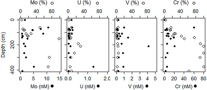
FIGURE 3. Groundwater depth profiles for concentrations (solid circles; lower axis) and percent of total dissolved metal (open circles; upper axis) associated with hydrophobic organic matter (as determined by extraction on a C18 column). Surface water concentrations are shown at 0 cm depth.
In the seasonal transects, samples with sulfide concentration >10 µM showed evidence of non-conservative removal (Figure 4A). Most non-sulfidic (shallow groundwater) samples fell within the conservative mixing area or slightly below with the exception of clear non-conservative excess in July. Molybdenum anomalies calculated at the MT profile were near zero in shallow groundwater (<100 cm), and the concentration anomaly dropped to below zero at 130–140 cm (Figure 5A).
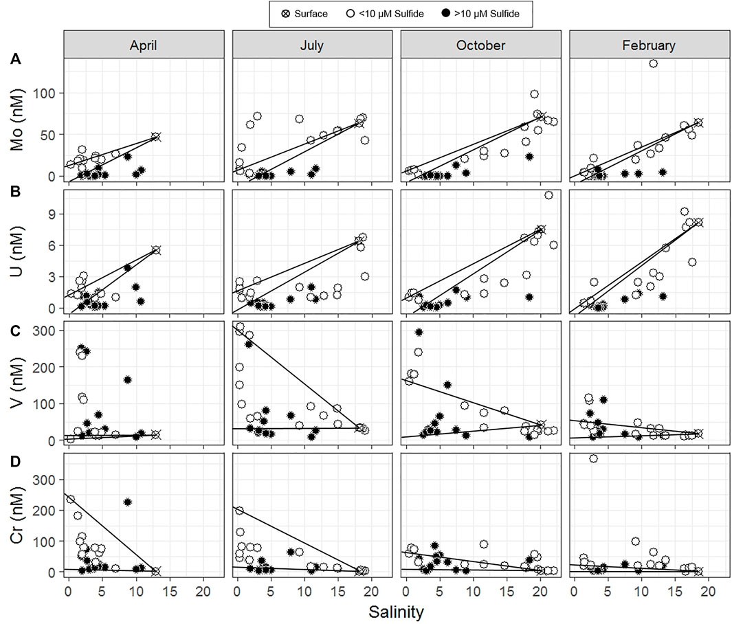
FIGURE 4. Salinity mixing diagrams of dissolved (A) Mo, (B) U, (C) V, and (D) Cr. Solid symbols indicate samples in which sulfide concentrations exceed 10 µM. Conservative mixing lines are drawn between the saline surface water endmember and both the deep and shallow freshwater endmembers (Table 1). Samples falling above and below the conservative mixing lines suggest non-conservative addition and removal, respectively.
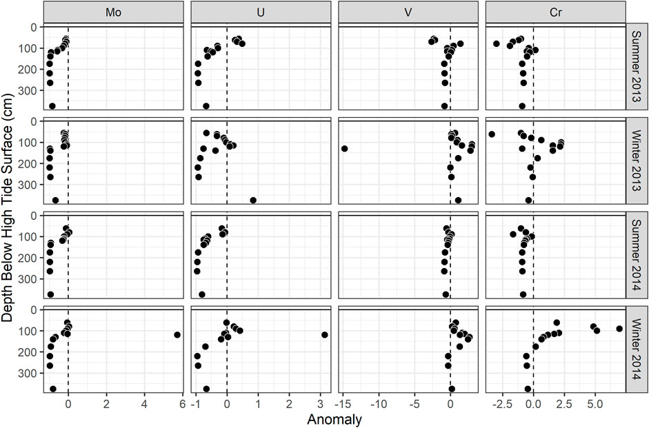
FIGURE 5. Concentration anomalies (calculated using three endmember mixing as described in the text) of (A) Mo, (B) U, (C) V, and (D) Cr at the MT profile. The points shown are the median anomaly values for each season.
The time effects linear model selected (based on AIC) for Mo was:
The models for individual seasons explained between 68 and 81% of the variability in Mo concentrations (Figure 6A). Molybdenum was correlated negatively with sulfide across all seasons. In seasons where the correlation with sulfide explained a lower percent of Mo variability (summer 2013 and winter 2014), the positive correlation with salinity was stronger.
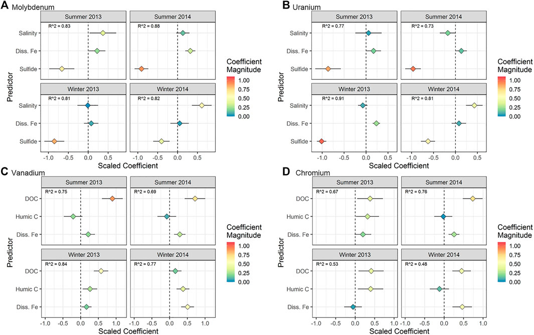
FIGURE 6. Regression results for (A) Mo, (B) U, (C) V, and (D) Cr for the time series taken at the MT sampling location (time effects). The horizontal axis represents the scaled coefficient for each predictor in the multiple linear regression (vertical axis). The color of the points shows the absolute magnitude of the coefficient. More extreme values (positive or negative) represent a stronger relationship between the predictor and the metal concentration. The horizontal line associated with each point represents the 95% confidence interval for the coefficient. For points where the confidence interval does not intersect 0, the p value for the coefficient is < 0.05.
The space effects linear model selected for Mo was the same as for the time effects model. The models for each location explained between 56 and 62% of the variability in Mo concentrations (Figure 7A). Salinity was the best predictor of Mo distribution at LT, whereas Fe and sulfide were better predictors at HT and MT, respectively.
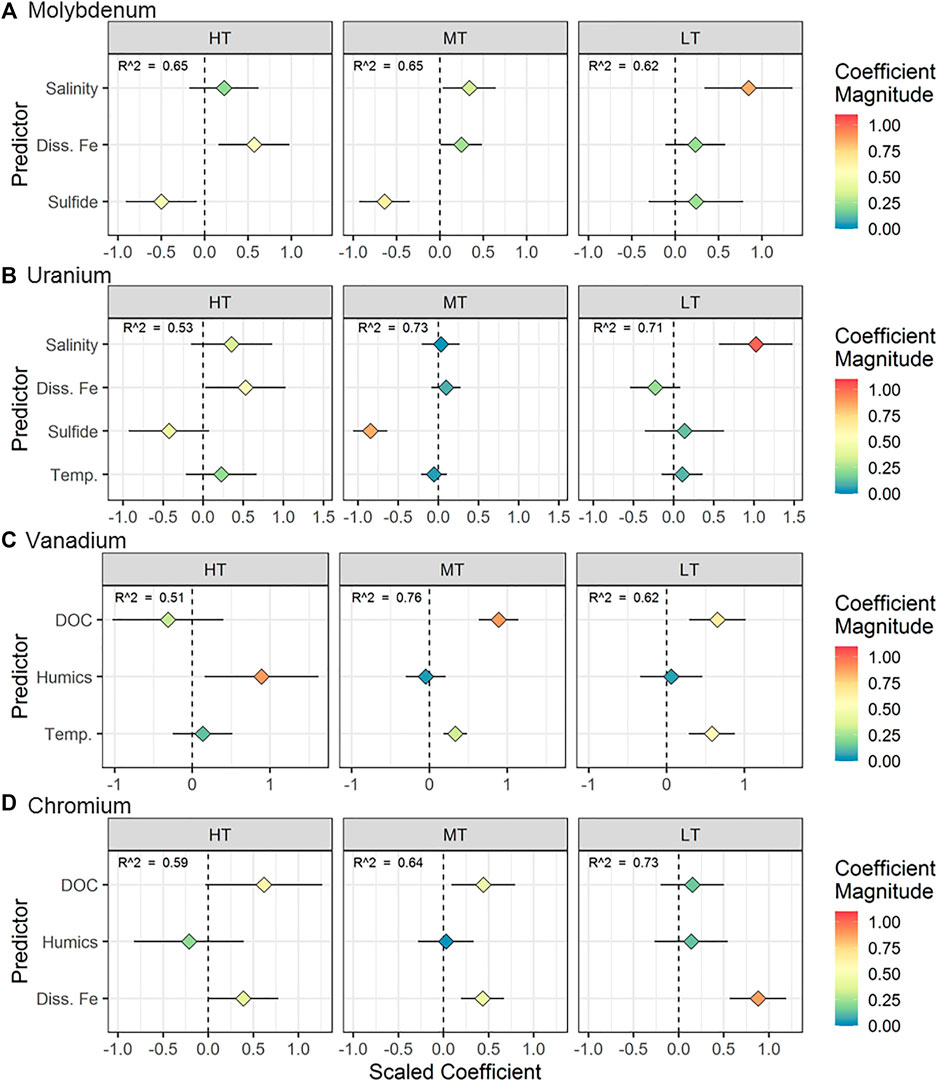
FIGURE 7. Regression results for (A) Mo, (B) U, (C) V, and (D) Cr for measurements taken along the STE transect (space effects). The horizontal axis represents the scaled coefficient for each predictor in the multiple linear regression (vertical axis). The color of the points shows the absolute magnitude of the coefficient. More extreme values (positive or negative) represent a stronger relationship between the predictor and the metal concentration. The horizontal line associated with each point represents the 95% confidence interval for the coefficient. For points where the confidence interval does not intersect 0, the p value for the coefficient is < 0.05.
3.1.2 Uranium
The mean U concentration for the shallow freshwater endmember (1.2 ± 0.6 nM) tended to be higher than that for the deep freshwater endmember (0.2 ± 0.2 nM), but both were much lower than estuarine surface water concentrations (7.2 ± 0.6 nM) (Table 1).
Dissolved U was highest in the surface water and shallowest parts of the STE. The 1 nM contour fell between 100 and 150 cm in July, and between 150 and 350 cm in February (Figure 1B). Summer U concentrations at MT remained relatively constant down to 90 cm (5 ± 3 nM), then decreased to <1 nM by 130 cm (Figure 2B). Winter U concentrations at MT remained relatively constant down to 100 cm (6 ± 4 nM), then decreased to <1 nM by 130 cm depth. At LT, U concentrations were consistently low (0.6 ± 0.6 nM), with somewhat higher concentrations evident at the shallowest (125 cm, 0.9 ± 0.2 nM) and deepest (300 cm, 1.6 ± 0.5 nM) sampled depths (Figure 1B). Concentrations of dissolved U associated with hDOM were relatively uniform (<0.5 nM) throughout the depth profile, with one sample reaching a maximum 1.4 nM between 300 and 400 cm depth (Figure 3B). The percent of U associated with hDOM was low in the surface (2.0%) and reached a maximum in the 200–300 cm depth range (15% ± 12) (Figure 3B).
In the seasonal transects, nearly all samples above salinity ∼3 showed non-conservative removal (in all months except April) (Figure 4B). Greater non-conservative behavior was observed in July than in other months based on the distance of points below the conservative mixing lines (Figure 4B) and the consistent negative concentration anomaly at shallower depths (Figure 5B). Uranium anomalies calculated at the MT were generally at or below zero from 62 to 115 cm, except in winter 2014, when anomalies were between zero and one, indicating enrichment (Figure 5B). Non-conservative removal occurred at all depths in summer 2013; at 90 cm and deeper in summer 2014; and at 140 cm and deeper in both winters. The anomalies calculated from three-endmember mixing typically fell between those calculated from mixing between the surface water and either the shallow or deep freshwater endmember.
The time effects linear model selected for U was:
The models for individual seasons explained between 54 and 84% of the variability in U concentrations (Figure 6B). The most statistically significant predictor of U concentrations over the 2-year sampling period was sulfide (negative correlation), followed by Fe (positive correlation) (Figure 6B). In winter 2014, the effect of Fe was not significant, but unlike other seasons, the effect of salinity was statistically significant.
The space effects linear model selected for U was:
The models for each location explained between 34 and 71% of the variability in U concentrations (Figure 7B). The best predictor of U concentration varied between locations. At HT, U was directly proportional to dissolved iron. At MT, U was inversely proportional to dissolved sulfide whereas salinity was the strongest predictor of U concentrations at LT (Figure 7B).
3.1.3 Vanadium
Dissolved V showed a mid-depth concentration maximum throughout the STE (Figure 1C). The maximum was generally between 50 and 250 cm from HT to MT, and 150–250 cm at LT. Dissolved V concentrations were highest from HT to MT and were never below the detection limit (2 nM) at any location. Within the MT profile maximum (from 100 to 140 cm), V concentrations ranged from a low of 147 ± 24 nM in winter 2014 to a high of 256 ± 54 nM in summer 2014 (Figure 2C), with generally higher concentrations in summer than in winter (Figures 1C,2C; Supplementary Figure S2). Concentrations of dissolved V associated with hDOM were typically 1–2 nM at all depths and the fraction of V associated with hDOM was low throughout the surface water and STE (<5%; Figure 3).
On average, vanadium was lowest in the deep freshwater endmember and highest in the shallow freshwater endmember (Table 1). The shallow freshwater endmember concentration was variable, increasing by a factor of six between April (2.48 nM) and July (296.9 nM). This shallow freshwater endmember was the primary source of V to the STE (having the highest concentration in all months but April). The deep freshwater endmember varied between a low of 8.8 nM in February to a high of 30.7 nM in July. Surface water concentrations varied between a low of 7.24 in February to a high of 42.1 in October.
In salinity mixing diagrams for the seasonal transects, V generally showed non-conservative addition, although patterns varied by month (Figure 4C). In July (with the highest shallow freshwater endmember concentration), most samples showed conservative behavior. In April and February (with lower shallow freshwater endmember concentrations), several sulfidic and non-sulfidic samples showed non-conservative addition. The calculated V anomalies at MT were primarily positive and were greatest between 100 and 175 cm in all seasons, coinciding with the mid-depth V concentration maximum. The concentration anomalies within the peak were higher in winter than in summer (Figure 5C). The anomalies within the V concentration maximum from three-endmember mixing typically were lower than those calculated from mixing between the surface water and the shallow or deep freshwater endmember.
The time effects linear model selected for V was:
The models for individual seasons explained between 67 and 83% of the variability in V concentrations (Figure 6C). Both DOC and Fe were directly correlated with V in most seasons (Figure 6C). Humic carbon was a significant predictor of V only in winter.
The space effects linear model selected for V was:
Models for each location explained between 40 and 74% of the variability in V concentration (Figure 7C). Dissolved organic carbon and temperature were positively correlated with V at MT and LT (Figure 7C), whereas V was significantly correlated with only humic carbon at HT. The direct correlation of V with temperature reflects the observed higher V concentrations in summer (Figures 1C,2C). Salinity was not a predictor of V in either the time effects or space effects models, which is consistent with only one of the freshwater endmembers acting as a primary source of V to the STE (as opposed to the existence of a single consistent fresh or saline source) (Table 1).
3.1.4 Chromium
Chromium was lowest in surface water (3 ± 3 nM) and highest in the shallow freshwater endmember (19.4–235.6 nM) (Table 1). Similar to V, Cr showed a mid-depth concentration maximum throughout the shallow STE (Figure 1D). Maximum Cr concentrations were observed from 90 to 130 cm depth at HT, from 100 to 200 cm depth at MT, and 125–150 cm at LT (Figure 1D). Concentrations of Cr were typically highest at HT, with concentrations commonly >100 nM, and up to 235 nM (Figure 1D). In the MT time series, Cr concentrations within the maximum ranged from 28 ± 3 nM in winter 2014 to a high of 53 ± 31 nM in winter 2013 (Figure 2D). Like V, Cr concentrations were always above the detection limit (1 nM). Concentrations of Cr within the maximum at MT did not show any consistent trends with season, but were higher during 2013 (Figure 2D, Supplementary Figure S2). Concentrations of dissolved Cr associated with hDOM were highest in the same depth range as the dissolved Cr maximum, between 100 and 200 cm depth (Figure 3). The percent of Cr associated with hDOM increased with depth in the STE from the surface water (2.8%) to the 301–410 cm depth interval (81% ± 26; Figure 3).
In salinity mixing diagrams for the seasonal transects, Cr concentrations generally exhibited conservative mixing behavior in the summer and non-conservative addition in the fall/winter when shallow freshwater endmember Cr concentrations were lower (Figure 4D). Additionally, positive Cr concentration anomalies (indicating addition) were observed at the MT profile, and tended to be higher in winter than summer (Figure 5D).
The time effects linear model selected for Cr was:
The models for individual seasons explained between 45 and 75% of the variability in Cr concentrations (Figure 6D). In 2013, Cr was positively correlated with DOC and humic carbon (Figure 6D). However, Cr was correlated with DOC and Fe (and not humic carbon) in 2014.
The space effects linear model selected for Cr was:
The models for each location explained between 55 and 71% of the variability in Cr concentrations (Figure 7D). Chromium was positively correlated with Fe at LT, and correlated with both DOC and Fe at MT. At HT, the predictor closest to statistical significance was Fe (p = 0.066). Similar to the linear models of V concentrations, salinity was not a predictor of Cr. However, unlike models for V, temperature was not a predictor of Cr concentrations, reflecting its more constant concentrations between summer and winter (Figure 2D).
3.2 Sediment
Metal oxide-associated Mo content in sediments was low (<1.5 μmol/cm3) in the shallowest sediments, increased to ∼4 μmol/cm3 between 70 and 150 cm, then increased to reach as high as 7.8 µmol/cm3 at depth (Figure 8). Metal oxide-associated U was low (∼0.1 μmol/cm3) down to 45 cm depth, increased to 1–2 μmol/cm3 between 70 and 250 cm depth, then increased to 5 μmol/cm3 at the base of the profile. Recalcitrant Mo and U profiles showed similar distributions to their metal oxide fractions.
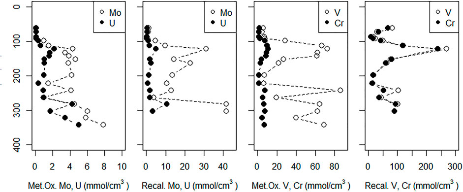
FIGURE 8. Sediment concentrations of metals dissolved by reducing (Metal Ox.) and aqua regia (recalcitrant [Recal.]) leaches (described in Methods). The sediment core was taken adjacent to the MT profile. The dotted line represents the sediment surface; depths are relative to the sediment surface at HT.
Metal oxide-associated V and Cr content were highest between 60–90 cm and 190–300 cm depths (Figure 8). Sediment concentrations of metal oxide-associated V reached as high as 86 μmol/cm3 while reducible Cr reached as high as 11 μmol/cm3. Recalcitrant V and Cr showed similar distributions as the metal oxide fractions, but with a sharper peak at 70 cm depth and similar concentrations.
4 Discussion
4.1 Molybdenum
High Mo concentrations in the surface water and shallow STE (compared to freshwater endmembers) showed Mo was supplied to the STE by estuary surface water (Figures 1A,2A). Once in STE groundwater, Mo was non-conservatively removed during advection into sulfidic portions of the STE (Figures 4A, 5A). Mo in sulfidic samples was always below concentrations expected for conservative mixing (Figure 4A), and calculated anomalies showed that Mo was consistently removed from groundwater where dissolved sulfide was first present, between 100 and 140 cm depth at MT (Figure 4A; O'Connor et al., 2018). These results are consistent with Mo observations from other STEs globally. Non-conservative removal of molybdenum was observed in several other study sites on the Atlantic and North Sea coasts (Windom and Niencheski 2003; Beck et al., 2008; Reckhardt et al., 2017). Reckhardt et al. (2017) demonstrated that Mo and sulfate depletion were correlated.
Measuring sulfide and using statistical modelling provided quantitative support for previous hypotheses regarding sulfide control on the removal of Mo. Multiple linear regression confirmed a negative correlation between Mo and sulfide throughout the STE (with the exception of the low tide location, discussed below) in all seasons (Figures 6A,7A). Laboratory and field studies suggest that at a sulfide threshold of ∼10 µM a geochemical “switch” is flipped and molybdate quantitatively reacts to form highly particle reactive thiomolybdate (MoS42-) (Helz et al., 1996; Erickson and Helz 2000). In this work, we confirm Mo removal primarily occurs where sulfide is present at concentrations higher than 10 µM (Figure 4A), consistent with these laboratory results. The negative correlation between Mo and sulfide throughout the 2-year time series suggests the importance of Mo removal by sulfide in every season (Figure 6A).
Sulfide concentrations varied seasonally in this STE (O'Connor et al., 2018), with higher concentrations during summer in the depth range where Mo was removed (100–140 cm; Figure 5A). However, Mo removal did not appear to be more extensive in summer (Figures 4A,5A). This may be because sulfide reached sufficiently high concentrations to drive Mo removal (>10 µM) by 140 cm depth in all seasons (O'Connor et al., 2018). Seasonal removal of Mo is more likely to occur in STEs where sulfide concentrations vary around a low-micromolar concentration threshold (e.g., Beck et al., 2008; Morford et al., 2009).
Sediment Mo content was consistent with Mo removal from groundwater to form insoluble compounds. Both metal oxide-associated and recalcitrant Mo increased in the 100–140 cm depth range (Figure 8) where sulfide and Mo co-occurred and dissolved Mo was removed (Figure 5A). Sediment Mo contents also increased with depth (Figure 8) suggests that the Mo-sulfide interface may shift over time, resulting in thiomolybdate compounds sorbing to sediments at different depths.
The pattern of Mo removal differed spatially throughout the STE. At LT, lower Mo concentrations and stronger correlation of Mo with salinity (Figure 7A) suggested that Mo removal typically occurs at shallow enough depths (sulfide concentrations were >250 μM at every sampled depth; O'Connor et al., 2018) that increasingly reducing conditions at depth did not drive further changes in Mo. This observation suggests that more seaward portions of shallow STEs may act as a greater Mo sink than intertidal zones.
Modeling done in this study supports a potential mechanism for Mo mobilization from the shallow STE observed by Beck et al. (2010) and in several samples in this study. Because molybdate can sorb to Mn oxides under oxic conditions (Shimmield and Price 1986), Beck et al. (2010) suggested that this may be associated with mobilization of metal (particularly Mn) oxides. This study confirms that dissolved Fe and Mo are correlated in summer months and that metal oxide-associated Mo occurs in shallow STE sediments (Figure 8), supporting the hypothesis that under non-sulfidic conditions, Mo cycling may be seasonally controlled by Fe and/or Mn oxidation and reductive dissolution (described in O’Connor et al., 2018).
The distribution of Mo contents in the groundwater and sediment suggests there may be spatial differences in the permanence of sequestration. Increasing concentrations of Mo in sediment occur near the redox interface, and may be mobilized with mixing of saline and oxic surface water into the STE. This mixing depends on the hydraulic gradient between groundwater and surface water (Gonneea et al., 2013; Luek and Beck 2014), which may be disturbed by short-term events such as storm surges or long-term events such as sea level rise. The highest concentrations of Mo in sediment occur at depth, where oxygen intrusion and remobilization are less likely.
4.2 Uranium
Consistent with many other studies (Duncan and Shaw 2003; Windom and Niencheski 2003; Charette and Sholkovitz 2006; Beck et al., 2008; Riedel et al., 2011; Reckhardt et al., 2017), uranium was supplied to the Gloucester Point STE by surface water and showed non-conservative removal with depth (Figures 1B, 2B, 4B, 5B). Sampling over several years and seasons showed that non-conservative removal was greater in summer. This is demonstrated by concentrations falling farther below the conservative mixing range in summer (Figure 4B) and shallower removal depths in the summer than the winter (Figure 5B).
Previous work has found inverse correlations between U and Fe, Mn, and sulfate reduction rate (Riedel et al., 2011; Reckhardt et al., 2017). This inverse relationship is consistent with U reduction coupled to metal oxide or sulfate reduction. Several microbial species, including many iron-reducing bacteria and sulfate/sulfur-reducing bacteria, (e.g., Geobacter metallireducens strain GS-15, Alteromonas putrefaciens, Shewanella putrefaciens, Desulfovibrio desulfuricans, Desulfovibrio vulgaris), can reduce U to its particle reactive species (Lovley et al., 1991; Lovley and Phillips 1992; Lovley et al., 1993; Fredrickson et al., 2000).
This work expands on these observations by assessing the relative importance of geochemical factors for U removal. Quantifying the relationship between U and other chemical parameters using multiple linear regression, rather than separate regressions, allowed for concurrent assessment of possible influences on U distribution. At the Gloucester Point STE, U was consistently inversely correlated with sulfide, while it showed either no correlation or a positive correlation with Fe (Figures 6B,7B). This suggests that sulfate/sulfur-reducing bacteria played a greater role in U reduction compared to iron-reducing bacteria at this STE. More extensive U removal in summer may be due to increased activity of sulfate/sulfur-reducing bacteria during warmer temperatures, which is consistent with conclusions drawn in O’Connor et al. (2018).
Similar to Mo, salinity exerted a stronger control on U concentrations at LT than at other locations in this STE (Figure 7B). Because redox conditions are largely consistent with depth at LT, U exhibits more conservative behavior compared to parts of the STE with more distinct redox gradients. Despite the strongly reducing conditions observed within the LT profile and consistently low U concentrations, U concentrations were always above the detection limit. Complexation with inorganic or organic ligands, which are both abundant throughout this STE, has been shown to inhibit the rate of microbially-mediated U reduction (Ganesh et al., 1997; Ganesh et al., 1999) and may therefore have led to the presence of soluble U within reducing groundwater.
Although both metal oxide-associated and recalcitrant U increased steadily with sediment depth (Figure 8), there was no U peak indicating a single clear depth of removal (as observed by Charette et al., 2005). Additionally, the increase in sediment U content was not as dramatic as the increase of Mo, despite similar contents in shallow (<100 cm) sediments. This may indicate that U removed to the sediments is more susceptible to remobilization during temporary increases in groundwater redox potential.
4.3 Vanadium
Dissolved V concentrations in the STE were highest mid-depth, evidently originating from shallow fresh groundwater (Figure 2C). Vanadium concentrations within the maximum (Figure 2C) and throughout the STE (Figure 1C) were highest in summer. These high summer concentrations appear partly due to higher concentrations of V in the shallow freshwater endmember (Table 1). A similar spatial and temporal pattern was observed in a tidal flat by Beck et al. (2008).
Dissolved V tends to be highest in groundwaters that are oxidizing and slightly basic (Wright and Belitz 2010; Pourret et al., 2012), unlike the reducing conditions throughout large portions of this and other coastal groundwater sites where high concentrations of V were measured in fresh water (Beck et al., 2008; Reckhardt et al., 2017). These studies found that V tends to be associated with higher DOC in reducing waters. Our multiple linear regression to model V concentrations found that V was correlated with both DOC and Fe throughout the 2-year time series (Figure 6A), suggesting that complexation by an inorganic-organic colloidal phase may have kept particle reactive reduced V species soluble (Pourret et al., 2012; Telfeyan et al., 2015). Only a small percent of V measured was in the hDOM pool at the Gloucester Point STE (Figure 3C). Therefore, hydrophilic organic matter (such as fulvic acids) may be important for complexation of V at this site (Stolpe et al., 2013; Telfeyan et al., 2015).
Higher V concentrations and higher DOC concentrations occurred in summer both at the Gloucester Point STE and the tidal flat studied in Beck et al. (2008). As proposed by Beck et al. (2008), this may be due to higher microbial activity in summer generating more labile organic compounds capable of complexing V. Our models found that the pool of organic matter associated with high V concentrations was different in the summer (correlated with DOC) versus the winter (correlated with humic carbon) (Figure 6A). This result suggests that, seasonal differences in organic matter concentration and composition could also drive seasonal changes in V concentration, and therefore mobility and eventual flux to the coastal ocean.
In addition to the seasonal variations in meteoric V supply, non-conservative addition of V occurred within the STE itself. Although higher V concentrations occurred in summer, greater non-conservative addition occurred during winter in both years (shown in seasonal transects and MT anomalies; Figures 4C,5C). Reduced V can sorb to hydrous metal oxides (Wehrli and Stumm 1989), and V was correlated with dissolved Fe in both winters (Figure 6C) at MT (Figure 7C). This is consistent with V release during the dissolution of Fe oxides, which occurs just up-gradient of the MT profile (O'Connor et al., 2018). These results suggest that the magnitude of the STE as a V source to the ocean depends on both organic matter source and seasonal redox dynamics.
The primary source of high V in the Gloucester Point STE may be local environmental factors. In inland groundwaters, V tends to be highest in aquifers composed of mafic and ultramafic rocks (Aiuppa et al., 2003; Wright and Belitz 2010; Luengo-Oroz et al., 2014). Sediments in the Chesapeake Bay region are rich in mafic and ultramafic minerals such as ilmenite, epidote, and staurolite (Firek et al., 1977; Darby 1984; Carpenter and Carpenter 1991). Additionally, fossil fuels can contribute to increased V concentrations in the environment (Andrade et al., 2004; Fiedler et al., 2008; Moreno et al., 2011), and coal burning emissions are a major source of contamination to sediments in the Chesapeake Bay region (Dickhut et al., 2000).
4.4 Chromium
Cr (like V) is enriched in minerals associated with mafic and ultramafic rock and in fossil fuels Robles-Camacho and Armienta, 2000 and Oze et al., 2007, which may provide the source of high Cr concentrations in fresh groundwater observed at the Gloucester Point STE. Cr concentrations were highest in a mid-depth maximum originating from shallow fresh groundwater (Figure 1D) and in the shallow freshwater endmember (Table 1). A similar distribution was observed in a tidal flat by Beck et al. (2008). The presence of dissolved Cr under reducing conditions is unusual given that soluble Cr(VI) is readily reduced to insoluble Cr(III) by Fe(II) (Eary and Rai 1989), organic matter (Bartlett and Kimble, 1976), and sulfide (Smillie et al., 1981), all of which are abundant in the Gloucester Point STE. Additionally, previous equilibrium calculations predict that Cr is reduced and therefore highly particle reactive throughout the STE (O'Connor et al., 2015). Beck et al. (2008) found a correlation between DOC and Cr and proposed that complexation with organic matter kept reduced Cr in solution (Bartlett and James 1983).
The multiple linear regression models for Cr offer more details regarding Cr complexation in the STE. At MT, Cr was correlated with DOC, supporting the hypothesis that complexation with organic matter can solubilize Cr in the STE. At MT, Cr was correlated with either humic carbon (in 2013) or Fe (in 2014) along with DOC (Figure 7D). In groundwater, colloids (small particles made up of aluminosilicate, iron (hydr)oxide, and organic components; Buffle et al., 1998) can enhance the transport of particle-reactive metals (Sanudo-Wilhelmy et al., 2002; De Jonge et al., 2004; Kim and Kim 2015). The correlation of Cr with both organic material and Fe at HT and MT suggested either that both Fe and Cr are present in organic complexes (Boggs et al., 1985), or that Cr is bound to mixed organic/inorganic colloidal material. However, Fe was the exclusive and strongest predictor at LT (Figure 7D). Colloids based on solid iron oxide material, rather than organic matter, are mobilized at oxic/anoxic interfaces and can transport metals (Pokrovsky and Schott 2002; Hassellov and von der Kammer 2008). As a result, the occurrence of sharp redox interfaces in the STE, including reductive dissolution of Fe oxides (O'Connor et al., 2015), may mobilize Fe-based colloids. This mobilization of Fe colloids may result in a shift from DOC- to Fe-mediated Cr transport moving seaward and shows that colloidal iron may play an important role for metal transport in addition to colloidal organic matter.
Unlike the other redox-active metals in this study, Cr showed interannual, rather that seasonal, variability in concentration. Interannual differences in the association of Cr with DOC, humic carbon, and Fe (Figure 6D) may have also contributed to interannual variability in groundwater Cr concentrations. Along with DOC, humic carbon predicted Cr concentrations in 2013, whereas Fe was the significant predictor in 2014, indicating a change in the composition of the material to which Cr was bound. A shift in composition could change binding constants or Cr solubility, resulting in increased concentrations. However, interannual variability was not observed for V. Compared with V, Cr was more strongly associated with the hDOM pool (Figure 3D), suggesting that distinct pools of dissolved organic matter complex V and Cr, which may account for differences in seasonal and interannual variability.
Despite not showing differences in concentration with season, Cr showed seasonally dependent non-conservative addition (Figures 4D,5D). Similar to V, non-conservative addition of Cr was greater in the winter. Because Cr species can sorb to reactive metal (hydr)oxide surfaces, this addition may be due to release upon reductive dissolution of Fe oxides, which is greater in winter in this STE (O'Connor et al., 2018).
5 Conclusion
Despite having similar chemical properties, Mo, U, V, and Cr behave differently in the STE due to differences in their sources within the STE and distinct biogeochemical properties. These differences cause seasonal variations in the concentrations and distributions of these elements in coastal groundwater at this study site.
Dissolved Mo and U were supplied to the STE by estuarine surface water and showed non-conservative removal when oxic surface water mixed into the reducing portions of the shallow STE. Molybdenum was removed by reaction with sulfide, but sulfide concentrations at this site were sufficiently high (i.e., in great excess of the 10 µM required to quantitatively react with Mo) that seasonal trends in removal were not evident. In contrast, U removal appeared linked to the activity of sulfate/sulfur-reducing bacteria and showed greater removal during summer (when temperatures are warmer and microbial metabolic rates are higher).
Both V and Cr were primarily supplied to the STE by meteoric groundwater and showed non-conservative addition within the STE. Minerals common to sediments in the region are enriched in V and Cr and were the most likely source of these elements to local groundwater. The mobility of V and Cr within the STE, and therefore their supply to the coastal ocean, was controlled by association/complexation with groundwater organic matter and Fe-rich colloids. Complexation with different organic matter pools may have led to seasonal variability in the distribution of V, but greater interannual variability of Cr.
Results from this study emphasize the importance of seasonality on biogeochemical cycling in the STE. Although the broader redox structure of the shallow STE was stable over this 2-year study, the magnitude of its source/sink functions changed in predictable ways. For example, studying metals cycling at a seasonal scale revealed greater U removal in summer, which could lead to an overestimation of the STE as a U sink. By simultaneously measuring trace metal concentrations and major redox constituents, seasonal variability in V and Cr concentrations was observed, and these changes could be explained by concomitant variability in DOC and Fe. This result also illustrates that easily measured major redox species such as organic carbon and Fe, which vary seasonally in other STEs, can help explain and even predict the behavior of redox-active trace metals. Understanding these seasonal changes in the distribution of RSMs within the STE can contribute to more accurate estimates of regional or global SGD-driven fluxes of heavy metals.
Data Availability Statement
The original contributions presented in the study are included in the article/Supplementary Material, further inquiries can be directed to the corresponding author.
Author Contributions
AO and AB contributed to the conception, design, and execution of this study. AO performed the statistical analysis. All authors contributed to manuscript preparation and revision, read, and approved the submitted version.
Funding
This work was supported by the National Science Foundation Graduate Research Fellowship Program (grant no: DGE-1444317) and the Virginia Institute of Marine Science.
Conflict of Interest
Author AO was employed by company Ramboll.
The remaining authors declare that the research was conducted in the absence of any commercial or financial relationships that could be construed as a potential conflict of interest.
Publisher’s Note
All claims expressed in this article are solely those of the authors and do not necessarily represent those of their affiliated organizations, or those of the publisher, the editors and the reviewers. Any product that may be evaluated in this article, or claim that may be made by its manufacturer, is not guaranteed or endorsed by the publisher.
Acknowledgments
The authors would like to thank Julie Krask, Leah Fitchett, and Michele Cochran for their invaluable help in the field and laboratory, and Alan Shiller for sample analyses. This article is Contribution 4069 of the Virginia Institute of Marine Science, William and Mary.
Supplementary Material
The Supplementary Material for this article can be found online at: https://www.frontiersin.org/articles/10.3389/fenvs.2021.613191/full#supplementary-material
References
Aiuppa, A., Bellomo, S., Brusca, L., D'Alessandro, W., and Federico, C. (2003). Natural and Anthropogenic Factors Affecting Groundwater Quality of an Active Volcano (Mt. Etna, Italy). Appl. Geochem. 18, 863–882. doi:10.1016/s0883-2927(02)00182-8
Algeo, T. J., Morford, J., and Cruse, A. (2012). Reprint of: New Applications of Trace Metals as Proxies in Marine Paleoenvironments. Chem. Geology. 324-325, 1–5. doi:10.1016/j.chemgeo.2012.07.012
Andrade, L., Marcet, P., Fernández-Feal, L., Fernández-Feal, C., Covelo, E., and Vega, F. (2004). Impact of the Prestige Oil Spill on Marsh Soils: Relationship between Heavy Metal, Sulfide and Total Petroleum Hydrocarbon Contents at the Villarrube and Lires Marshes (Galicia, Spain). Cienc. Mar. 30, 477–487. doi:10.7773/cm.v30i3.281
Anschutz, P., Dedieu, K., Desmazes, F., and Chaillou, G. (2005). Speciation, Oxidation State, and Reactivity of Particulate Manganese in marine Sediments. Chem. Geol. 218, 265–279. doi:10.1016/j.chemgeo.2005.01.008
Anschutz, P., Smith, T., Mouret, A., Deborde, J., Bujan, S., Poirier, D., et al. (2009). Tidal Sands as Biogeochemical Reactors. Estuar. Coast. Shelf Sci. 84, 84–90. doi:10.1016/j.ecss.2009.06.015
Archer, C., and Vance, D. (2008). The Isotopic Signature of the Global Riverine Molybdenum Flux and Anoxia in the Ancient Oceans. Nat. Geosci. 1, 597–600. doi:10.1038/ngeo282
Barnes, C. E., and Cochran, J. K. (1993). Uranium Geochemistry in Estuarine Sediments: Controls on Removal and Release Processes. Geochim. Cosmochim. Acta 57, 555–569. doi:10.1016/0016-7037(93)90367-6
Bartlett, R. J., and Kimble, J. M. (1976). Behavior of Chromium in Soils: II. Hexavalent Forms. J. Environ. Quality 5, 383–386. doi:10.2134/jeq1976.00472425000500040010x
Bartlett, R. J., and James, B. (1983). Behavior of Chromium in Soils: V. Fate of Organically Complexed Cr(III) Added to Soil. J. Environ. Qual. 12, 169–172. doi:10.2134/jeq1983.00472425001200020003x
Beck, A. J., Tsukamoto, Y., Tovar-Sanchez, A., Huerta-Diaz, M., Bokuniewicz, H. J., and Sañudo-Wilhelmy, S. A. (2007). Importance of Geochemical Transformations in Determining Submarine Groundwater Discharge-Derived Trace Metal and Nutrient Fluxes. Appl. Geochem. 22, 477–490. doi:10.1016/j.apgeochem.2006.10.005
Beck, M., Dellwig, O., Schnetger, B., and Brumsack, H-J. (2008). Cycling of Trace Metals (Mn, Fe, Mo, U, V, Cr) in Deep Pore Waters of Intertidal Flat Sediments. Geochim. Cosmochim. Acta 72 (12), 2822–2840. doi:10.1016/j.gca.2008.04.013
Beck, A. J., Cochran, J. K., and Sañudo-Wilhelmy, S. A. (2009). Temporal Trends of Dissolved Trace Metals in Jamaica Bay, NY: Importance of Wastewater Input and Submarine Groundwater Discharge in an Urban Estuary. Estuaries Coasts 32, 535–550. doi:10.1007/s12237-009-9140-5
Beck, A. J., Cochran, J. K., and Sañudo-Wilhelmy, S. A. (2010). The Distribution and Speciation of Dissolved Trace Metals in a Shallow Subterranean Estuary. Mar. Chem. 121, 145–156. doi:10.1016/j.marchem.2010.04.003
Beck, A. J., Kellum, A. A., Luek, J. L., and Cochran, M. A. (2016). Chemical Flux Associated with Spatially and Temporally Variable Submarine Groundwater Discharge, and Chemical Modification in the Subterranean Estuary at Gloucester Point, VA (USA). Estuaries Coasts 39, 1–12. doi:10.1007/s12237-015-9972-0
Behrends, T., and Van Cappellen, P. (2005). Competition between Enzymatic and Abiotic Reduction of Uranium(VI) under Iron Reducing Conditions. Chem. Geol. 220, 315–327. doi:10.1016/j.chemgeo.2005.04.007
Boggs, S., Livermore, D., and Seitz, M. G. (1985). Humic Substances in Natural Waters and Their Complexation with Trace Metals and Radionuclides: A Review. IL (USA): Argonne National Lab.
Bruland, K. W., and Lohan, M. C. (2006). “Controls of Trace Metals in Seawater,” in The Oceans and Marine Geochemistry. Editors H. D. Hollands, K. K. Turekian, and H. Elderfield (Oxford: Elsevier), 23–47.
Brumsack, H. J., and Gieskes, J. M. (1983). Interstitial Water Trace-Metal Chemistry of Laminated Sediments from the Gulf of California, Mexico. Mar. Chem. 14, 89–106. doi:10.1016/0304-4203(83)90072-5
Buffle, J., Wilkinson, K., Stoll, S., Filella, M., and Zhang, J. (1998). A generalized Description of Aquatic Colloidal Interactions: The Three-Colloidal Component Approach. Environ. Sci. Technol. 32, 2887–2899. doi:10.1021/es980217h
Burnett, W. C., Bokuniewicz, H., Huettel, M., Moore, W. S., and Taniguchi, M. (2003). Groundwater and Pore Water Inputs to the Coastal Zone. Biogeochem 66, 3–33. doi:10.1023/b:biog.0000006066.21240.53
Burnett, W. C., Peterson, R., Moore, W. S., and de Oliveira, J. (2008). Radon and Radium Isotopes as Tracers of Submarine Groundwater Discharge - Results From the Ubatuba, Brazil SGD Assessment Intercomparison. Estuar. Coast. Shelf Sci. 76, 501–511. doi:10.1016/j.ecss.2007.07.027
Cable, J. E., Burnett, W. C., Chanton, J. P., and Weatherly, G. L. (1996). Estimating Groundwater Discharge into the Northeastern Gulf of Mexico Using Radon-222. Earth Planet. Sci. Lett. 144, 591–604. doi:10.1016/S0012-821X(96)00173-2
Carpenter, R. G., and Carpenter, S. F. (1991). Heavy mineral Deposits in the Upper Coastal plain of North Carolina and Virginia. Econ. Geol. 86, 1657–1671. doi:10.2113/gsecongeo.86.8.1657
Charette, M. A., and Sholkovitz, E. R. (2006). Trace Element Cycling in a Subterranean Estuary: Part 2. Geochemistry of the Pore Water. Geochim. Cosmochim. Acta 70, 811–826. doi:10.1016/j.gca.2005.10.019
Charette, M. A., Sholkovitz, E. R., and Hansel, C. M. (2005). Trace Element Cycling in a Subterranean Estuary: Part 1. Geochemistry of the Permeable Sediments. Geochim. Cosmochim. Acta 69, 2095–2109. doi:10.1016/j.gca.2004.10.024
Darby, D. A. (1984). Trace Elements in Ilmenite: A Way to Discriminate Provenance or Age in Coastal Sands. Geol. Soc. Am. Bull. 95, 1208–1218. doi:10.1130/0016-7606(1984)95<1208:teiiaw>2.0.co;2
de Jonge, L. W., Klaergaard, C., and Moldrup, P. (2004). Colloids and Colloid Facilitated Transport of Contaminants in Soils: An Introduction. Vadose Zo. J. 3, 321–325. doi:10.2136/vzj2004.0321
Dickhut, R. M., Canuel, E. A., Gustafson, K. E., Liu, K., Arzayus, K. M., Walker, S. E., et al. (2000). Automotive Sources of Carcinogenic Polycyclic Aromatic Hydrocarbons Associated with Particulate Matter in the Chesapeake Bay Region. Environ. Sci. Technol. 34, 4635–4640. doi:10.1021/es000971e
Duncan, T., and Shaw, T. J. (2003). The Mobility of Rare Earth Elements and Redox Sensitive Elements in the Groundwater/Seawater Mixing Zone of a Shallow Coastal Aquifer. Aquat. Geochem. 9, 233–255. doi:10.1023/b:aqua.0000022956.20338.26
Eary, L. E., and Rai, D. (1989). Kinetics of Chromate Reduction by Ferrous Ions Derived from Hematite and Biotite at 25°C. Am. J. Sci. 289, 180–213.
Erickson, B. E., and Helz, G. R. (2000). Molybdenum (VI) Speciation in Sulfidic Waters: Stability and Lability of Thiomolybdates. Geochim. Cosmochim. Acta 64, 1149–1158. doi:10.1016/s0016-7037(99)00423-8
Fiedler, S., Siebe, C., Herre, a., Roth, B., Cram, S., and Stahr, K. (2008). Contribution of Oil Industry Activities to Environmental Loads of Heavy Metals in the Tabasco Lowlands, Mexico. Water Air Soil Pollut. 197, 35–47. doi:10.1007/s11270-008-9789-6
Firek, F., Shideler, G. L., and Fleischer, P. (1977). Heavy-Mineral Variability in Bottom Sediments of the Lower Chesapeake Bay, VA. Mar. Geol. 23, 217–235. doi:10.1016/0025-3227(77)90020-2
Fredrickson, J. K., Zachara, J. M., Kennedy, D. W., Duff, M. C., Gorby, Y. A., Li, S.-M. W., et al. (2000). Reduction of U(VI) in Goethite (Alpha-FeOOH) Suspensions by a Dissimilatory Metal-Reducing Bacterium. Geochim. Cosmochim. Acta 64, 3085–3098. doi:10.1016/s0016-7037(00)00397-5
Ganesh, R., Robinson, K. G., Reed, G. D., and Sayler, G. S. (1997). Reduction of Hexavalent Uranium from Organic Complexes by Sulfate- and Iron-Reducing Bacteria. Appl. Environ. Microbiol. 63, 4385–4391. doi:10.1128/aem.63.11.4385-4391.1997
Ganesh, R., Robinson, K. G., Chu, L., Kucsmas, D., and Reed, G. D. (1999). Reductive Precipitation of Uranium by Desulfovibri Desulfuricans: Evaluation of Co-contaminant Effects and Selective Removal. Wat. Res. 33, 3447–3458. doi:10.1016/s0043-1354(99)00024-x
Gonneea, M. E., Mulligan, A. E., and Charette, M. A. (2013). Seasonal Cycles in Radium and Barium within a Subterranean Estuary: Implications for Groundwater Derived Chemical Fluxes to Surface Waters. Geochim. Cosmochim. Acta 119, 164–177. doi:10.1016/j.gca.2013.05.034
Hassellov, M., and von der Kammer, F. (2008). Iron Oxides as Geochemical Nanovectors for Metal Transport in Soil-River Systems. Elements 4, 401–406. doi:10.2113/gselements.4.6.401
Helz, G. R., Miller, C. V., Charnock, J. M., Mosselmans, J. F. W., Pattrick, R. A. D., Garner, C. D., et al. (1996). Mechanism of Molybdenum Removal from the Sea and its Concentration in Black Shales: EXAFS Evidence. Geochim. Cosmochim. Acta 60, 3631–3642. doi:10.1016/0016-7037(96)00195-0
Hua, B., Xu, H., Terry, J., and Deng, B. (2006). Kinetics of Uranium(VI) Reduction by Hydrogen Sulfide in Anoxic Aqueous Systems. Environ. Sci. Technol. 40, 4666–4671. doi:10.1021/es051804n
Huerta-Diaz, M. A., and Morse, J. W. (1992). Pyritization of Trace Metals in Anoxic marine Sediments. Mar. Chem. 29, 119–144. doi:10.1016/0016-7037(92)90353-k
Hyacinthe, C., Bonneville, S., and Van Cappellen, P. (2006). Reactive Iron(III) in Sediments: Chemical versus Microbial Extractions. Geochim. Cosmochim. Acta 70, 4166–4180. doi:10.1016/j.gca.2006.05.018
James, G., Witten, D., Hastie, T., and Tibshirani, R. (2014). An Introduction to Statistical Learning: With Applications in R. New York: Springer Publishing Company, Incorporated.
Kim, I., and Kim, G. (2015). Role of Colloids in the Discharge of Trace Elements and Rare Earth Elements from Coastal Groundwater to the Ocean. Mar. Chem. 176, 126–132. doi:10.1016/j.marchem.2015.08.009
Klinkhammer, G. P., and Palmer, M. R. (1991). Uranium in the Oceans: Where it Goes and Why. Geochim. Cosmochim. Acta 55, 1799–1806. doi:10.1016/0016-7037(91)90024-y
Lemaire, E., Blanc, G., Coynel, A., and Etcheber, H. (2006). Dissolved Trace Metal – Organic Complexes in the Lot – Garonne River System Determined Using the C18 Sep-Pak System. Aquat. Geochem. 12, 21–38. doi:10.1007/s10498-005-0908-3
Lovley, D. R., and Phillips, E. J. P. (1992). Reduction of Uranium by Desulfovibrio Desulfuricans. Appl. Environ. Microbiol. 58, 850–856. doi:10.1128/aem.58.3.850-856.1992
Lovley, D. R., Phillips, E. J. P., Gorby, Y. A., and Landa, E. R. (1991). Microbial Reduction of Uranium. Nature 350, 413–416. doi:10.1038/350413a0
Lovley, D. R., Widman, P. K., Woodward, J. C., and Phillips, E. J. (1993). Reduction of Uranium by Cytochrome C3 of Desulfovibrio Vulgaris. Appl. Environ. Microbiol. 59, 3572–3576. doi:10.1128/aem.59.11.3572-3576.1993
Luek, J. L., and Beck, A. J. (2014). Radium Budget of the York River Estuary (VA, USA) Dominated by Submarine Groundwater Discharge with a Seasonally Variable Groundwater End-Member. Mar. Chem. 165, 55–65. doi:10.1016/j.marchem.2014.08.001
Luengo-Oroz, N., Bellomo, S., and D’Alessandro, W. (2014). “High Vanadium Concentrations in Groundwater at El Hierro (Canary Islands, Spain),” in 10th International Hydrogeological Congress, Thessalonik Greece, 8-10 October 2014, 427–435.
McAllister, S. M., Barnett, J. M., Heiss, J. W., Findlay, A. J., Macdonald, D. J., Dow, C. L., et al. (2015). Dynamic Hydrologic and Biogeochemical Processes Drive Microbially Enhanced Iron and Sulfur Cycling within the Intertidal Mixing Zone of a beach Aquifer. Limnol. Oceanogr. 60, 329–345. doi:10.1002/lno.10029
Moore, K. A., and Reay, W. G. (2009). CBNERRVA Research and Monitoring Program. J. Coast. Res. 57, 118–125. doi:10.2112/1551-5036-57.sp1.118
Moore, W. S. (1999). The Subterranean Estuary: a Reaction Zone of Ground Water and Sea Water. Mar. Chem. 65, 111–125. doi:10.1016/s0304-4203(99)00014-6
Moreno, R., Jover, L., Diez, C., and Sanpera, C. (2011). Seabird Feathers as Monitors of the Levels and Persistence of Heavy Metal Pollution after the Prestige Oil Spill. Environ. Pollut. 159, 2454–2460. doi:10.1016/j.envpol.2011.06.033
Morford, J. L., and Emerson, S. R. (1999). The Geochemistry of Redox Sensitive Trace Metals in Sediments. Geochim. Cosmochim. Acta 63, 1735–1750. doi:10.1016/s0016-7037(99)00126-x
Morford, J. L., Emerson, S. R., Breckel, E. J., and Kim, S. H. (2005). Diagenesis of Oxyanions (V, U, Re, and Mo) in Pore Waters and Sediments from a continental Margin. Geochim. Cosmochim. Acta 69, 5021–5032. doi:10.1016/j.gca.2005.05.015
Morford, J. L., Martin, W. R., François, R., and Carney, C. M. (2009). A Model for Uranium, Rhenium, and Molybdenum Diagenesis in marine Sediments Based on Results from Coastal Locations. Geochim. Cosmochim. Acta 73 (10), 2938–2960. doi:10.1016/j.gca.2009.02.029
Nameroff, T. J., Calvert, S. E., and Murray, J. W. (2004). Glacial-interglacial Variability in the Eastern Tropical North Pacific Oxygen Minimum Zone Recorded by Redox-Sensitive Trace Metals. Paleoceanography 19, 1–19. doi:10.1029/2003pa000912
O'Connor, A. E., Luek, J. L., McIntosh, H., and Beck, A. J. (2015). Geochemistry of Redox-Sensitive Trace Elements in a Shallow Subterranean Estuary. Mar. Chem. 172, 70–81. doi:10.1016/j.marchem.2015.03.001
O’Connor, A. E., Krask, J., Beck, A. J., and Canuel, E. (2018). Seasonality of Major Redox Constituents in a Shallow Subterranean Estuary. Geochim. Cosmochim. Acta 224, 344–361. doi:10.1016/j.gca.2017.10.013
Oze, C., Bird, D. K., and Fendorf, S. (2007). Genesis of Hexavalent Chromium from Natural Sources in Soil and Groundwater. PNAS 104, 6544–6549. doi:10.1073/pnas.0701085104
Pokrovsky, O., and Schott, J. (2002). Iron Colloids/organic Matter Associated Transport of Major and Trace Elements in Small Boreal Rivers and Their Estuaries (NW Russia). Chem. Geol. 190, 141–179. doi:10.1016/s0009-2541(02)00115-8
Pourret, O., Dia, A., Gruau, G., Davranche, M., and Bouhnik-Le Coz, M. (2012). Assessment of Vanadium Distribution in Shallow Groundwaters. Chem. Geol. 294–295, 89–102. doi:10.1016/j.chemgeo.2011.11.033
R Core Team (2015). R: A Language and Environment for Statistical Computing. Vienna, Austria: R Foundation for Statistical Computing. URL: https://www.R-project.org/.
Rai, D., Eary, L. E., and Zachara, J. M. (1989). Environmental Chemistry of Chromium. Sci. Total Environ. 86, 15–23. doi:10.1016/0048-9697(89)90189-7
Remoundaki, E., Hatzikioseyian, A., and Tsezos, M. (2007). A Systematic Study of Chromium Solubility in the Presence of Organic Matter: Consequences for the Treatment of Chromium-Containing Wastewater. J. Chem. Technol. Biotechnol. 82, 802–808. doi:10.1002/jctb.1742
Reckhardt, A., Beck, M., Greskowiak, J., Schnetger, B., Bӧttcher, M. E., Gehre, M., et al. (2017). Cycling of Redox-Sensitive Elements in a Sandy Subterranean Estuary of the Southern North Sea. Mar. Chem. 188, 6–17. doi:10.1016/j.marchem.2016.11.003
Riedel, T., Lettmann, K., Schnetger, B., Beck, M., and Brumsack, H.-J. (2011). Rates of Trace Metal and Nutrient Diagenesis in an Intertidal Creek Bank. Geochim. Cosmochim. Acta 75, 134–147. doi:10.1016/j.gca.2010.09.040
Rimmer, S. M., Thompson, J. a., Goodnight, S. a., and Robl, T. L. (2004). Multiple Controls on the Preservation of Organic Matter in Devonian–Mississippian marine Black Shales: Geochemical and Petrographic Evidence. Palaeogeogr. Palaeoclimatol. Palaeoecol. 215, 125–154. doi:10.1016/s0031-0182(04)00466-3
Robles-Camacho, J., and Armienta, M. A. (2000). Natural Chromium Contamination of Groundwater at Leon Valley, Mexico. J. Geochemical Explor. 68, 167–181. doi:10.1016/s0375-6742(99)00083-7
Santos, I. R., Burnett, W. C., Dittmar, T., Suryaputra, I. G. N. A., and Chanton, J. (2009). Tidal Pumping Drives Nutrient and Dissolved Organic Matter Dynamics in a Gulf of Mexico Subterranean Estuary. Geochim. Cosmochim. Acta 73, 1325–1339. doi:10.1016/j.gca.2008.11.029
Santos, I. R., Burnett, W. C., Misra, S., Suryaputra, I. G. N. A., Chanton, J. P., Dittmar, T., et al. (2011). Uranium and Barium Cycling in a Salt Wedge Subterranean Estuary: The Influence of Tidal Pumping. Chem. Geol. 287, 114–123. doi:10.1016/j.chemgeo.2011.06.005
Sañudo-Wilhelmy, S. A., Rossi, F. K., Bokuniewicz, H., and Paulsen, R. J. (2002). Trace Metal Levels in Uncontaminated Groundwater of a Coastal Watershed: Importance of Colloidal Forms. Environ. Sci. Technol. 36, 1435–1441. doi:10.1021/es0109545
Scholz, F., Hensen, C., Noffke, A., Rohde, A., Liebetrau, V., and Wallmann, K. (2011). Early Diagenesis of Redox-Sensitive Trace Metals in the Peru Upwelling Area – Response to ENSO-Related Oxygen Fluctuations in the Water Column. Geochim. Cosmochim. Acta 75, 7257–7276. doi:10.1016/j.gca.2011.08.007
Shimmield, G., and Price, N. (1986). The Behaviour of Molybdenum and Manganese during Early Sediment Diagenesis — Offshore Baja California, Mexico. Mar. Chem. 19, 261–280. doi:10.1016/0304-4203(86)90027-7
Siebert, C., Nägler, T. F., von Blanckenburg, F., and Kramers, J. D. (2003). Molybdenum Isotope Records as a Potential New Proxy for Paleoceanography. Earth Planet. Sci. Lett. 211, 159–171. doi:10.1016/s0012-821x(03)00189-4
Slomp, C. P., and Van Cappellen, P. (2004). Nutrient Inputs to the Coastal Ocean through Submarine Groundwater Discharge: Controls and Potential Impact. J. Hydrol. 295, 64–86. doi:10.1016/j.jhydrol.2004.02.018
Smillie, R. H., Hunter, K., and Loutit, M. (1981). Reduction of Chromium(VI) by Bacterially Produced Hydrogen Sulphide in a marine Environment. Water Res. 15, 1351–1354. doi:10.1016/0043-1354(81)90007-5
Snyder, M., Taillefert, M., and Ruppel, C. (2004). Redox Zonation at the saline-influenced Boundaries of a Permeable Surficial Aquifer: Effects of Physical Forcing on the Biogeochemical Cycling of Iron and Manganese. J. Hydrol. 296, 164–178. doi:10.1016/j.jhydrol.2004.03.019
Spinelli, G. A., and Fisher, A. T. (2002). Groundwater Seepage into Northern San Francisco Bay: Implications for Dissolved Metals Budgets. Water Resour. Res. 38, 12-1–12-19. doi:10.1029/2001wr000827
Stolpe, B., Guo, L., Shiller, A. M., and Aiken, G. R. (2013). Abundance, Size Distributions and Trace-Element Binding of Organic and Iron-Rich Nanocolloids in Alaskan Rivers, as Revealed by Field-Flow Fractionation and ICP-MS. Geochim. Cosmochim. Acta 105, 221–239. doi:10.1016/j.gca.2012.11.018
Telfeyan, K., Johannesson, K. H., Mohajerin, T. J., and Palmore, C. D. (2015). Vanadium Geochemistry along Groundwater Flow Paths in Contrasting Aquifers of the United States: Carrizo Sand (Texas) and Oasis Valley (Nevada) Aquifers. Chem. Geol. 410, 63–78. doi:10.1016/j.chemgeo.2015.05.024
Tessier, A., Campbell, P. G. C., and Bisson, M. (1979). Sequential Extraction Procedure for the Speciation of Particulate Trace Metals. Anal. Chem. 51, 844–851. doi:10.1021/ac50043a017
Tribovillard, N., Algeo, T. J., Lyons, T., and Riboulleau, A. (2006). Trace Metals as Paleoredox and Paleoproductivity Proxies: An Update. Chem. Geol. 232, 12–32. doi:10.1016/j.chemgeo.2006.02.012
Wanty, R. B., and Goldhaber, M. B. (1992). Thermodynamics and Kinetics of Reactions Involving Vanadium in Natural Systems: Accumulation of Vanadium in Sedimentary Rocks. Geochim. Cosmochim. Acta 56, 1471–1483. doi:10.1016/0016-7037(92)90217-7
Wehrli, B., and Stumm, W. (1989). Vanadyl in Natural Waters: Adsorption and Hydrolysis Promote Oxygenation. Geochim. Cosmochim. Acta 53, 69–77. doi:10.1016/0016-7037(89)90273-1
Windom, H., and Niencheski, F. (2003). Biogeochemical Processes in a Freshwater–Seawater Mixing Zone in Permeable Sediments along the Coast of Southern Brazil. Mar. Chem. 83, 121–130. doi:10.1016/s0304-4203(03)00106-3
Keywords: subterranean estuary, submarine groundwater discharge, coastal groundwater, redox-sensitive metals, oxyanion-forming elements
Citation: O'Connor AE, Canuel EA and Beck AJ (2022) Drivers and Seasonal Variability of Redox-Sensitive Metal Chemistry in a Shallow Subterranean Estuary. Front. Environ. Sci. 9:613191. doi: 10.3389/fenvs.2021.613191
Received: 01 October 2020; Accepted: 09 December 2021;
Published: 17 January 2022.
Edited by:
Clare Robinson, Western University, CanadaReviewed by:
Xueyan Jiang, Ocean University of China, ChinaGuebuem Kim, Seoul National University, South Korea
Gwénaëlle Chaillou, Université du Québec à Rimouski, Canada
Copyright © 2022 O'Connor, Canuel and Beck. This is an open-access article distributed under the terms of the Creative Commons Attribution License (CC BY). The use, distribution or reproduction in other forums is permitted, provided the original author(s) and the copyright owner(s) are credited and that the original publication in this journal is cited, in accordance with accepted academic practice. No use, distribution or reproduction is permitted which does not comply with these terms.
*Correspondence: Alison E. O'Connor, alisoneoconnor@gmail.com