Spatial Assessment of Water Use Efficiency (SDG Indicator 6.4.1) for Regional Policy Support

Introduction

The United Nations (UN) adopted an ambitious global sustainability agenda for the period up to 2030 (UN, 2015). In September 2015, heads of state and government from 193 member states of UN agreed to adopt the 2030 Agenda for Sustainable Development consisting of 17 goals and 169 targets (UN, 2017; UN-Water, 2018). Achieving the Sustainable Development Goals (SDGs) will require major efforts on how the monitoring of the progresses toward the goals can be tracked (UN, 2017; UN-Water, 2017b), and how consequent implementation actions can be identified and targeted to different situations (Gain et al., 2016). The multiplicity of essentially non-comparable measures of sustainable development necessitates the generation of “relevant” SDG indicators so that “clear, unambiguous messages be conveyed to users” (Hák et al., 2016). In this respect, there were attempts by their drafters, the UN Inter-Agency and Expert Group on SDG Indicators (IAEG-SDG), to ensure relevance. Although there are criticisms that many suggested indicators lack comprehensive, cross-country data and some even lack agreed statistical definitions (Schmidt-Traub et al., 2017), the United Nations Statistical Commission (UNSC) adopted a set of 230 indicators proposed by the IAEG-SDG on March 2016 as a practical starting point to monitor progress on the 17 goals and 169 targets of the SDGs (Allen et al., 2017).

Developing countries are usually those with the higher needs, bigger gaps between current capabilities and the targets and the more limited resources for accurate monitoring, due to limitations in the availability of information and in the statistical institutions to manage them (UN-Water, 2017a).

In order to move from agreeing on the goals to implementing and ultimately achieving them, Yonehara et al. (2017) suggested to divide the SDGs' 15-years time frame into three 5-years phases: a planning phase driven by proactive evaluation and evaluability assessment, an improvement phase characterized by formative evaluation and monitoring, and a completion phase involving outcome and impact evaluations (see Table 1). Reyers et al. (2017) and UN-Water (2016) stated that there must be greater attention on interlinkages across sectors (e.g., finance, agriculture, energy, and transport), across societal actors (local authorities, government agencies, private sector, and civil society), and across scales (Liu et al., 2017, 2018). In order to improve these interlinkages, Reyers et al. (2017) also provided seven recommendations pertaining to the following areas: finance, technology, capacity building, trade, policy coherence, partnerships, and, finally, data, monitoring and accountability. Among these seven recommendations, data collection, monitoring and accountability at different levels are highly important for the implementation of SDGs. Vanham et al. (2018) and FAO (2017), for example, suggested that SDGs implementation should be monitored at least three levels: national (e.g., country level), sub-national (e.g., basin level), and local level (see Table 2).

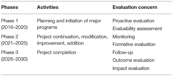
Table 1. Three 5-years phases for SDG implementation and evaluation, according to Yonehara et al. (2017).

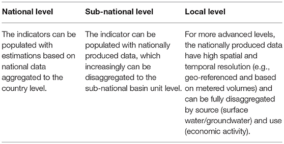
Table 2. Monitoring of SDG implementations at different levels, according to FAO (2017).

The main challenge for monitoring the implementation of the SDGs at national, sub-national and local levels remains in the availability of comparable global raw data collected with adequate spatial detail and quality at regular time intervals (Giupponi and Gain, 2017; Farinosi et al., 2018; UN-Water, 2018). Usually, country-level data are available globally from international organizations, such as the global water information system, AQUASTAT of the Food and Agriculture Organization (FAO). However, country-level averaging and aggregation hide the variability of physical and socio-economic phenomena (Gain et al., 2016). Therefore, the spatial detail is crucial to identify hot spot areas of greatest interest for planning the interventions toward the achievement of the SDGs (Giupponi and Gain, 2017; Farinosi et al., 2018). In addition, there is an urgent need for the research community to develop scientifically robust tools to help operationalize the SDGs at the global, regional, national and sub-national levels, with an aim to support the tracking of cross scale, local and aggregate, regional and global trends (Reyers et al., 2017). Specifically, quantitative assessments based on robust models and scenarios are required to foresight sustainable futures to back cast potential development pathways (Reyers et al., 2017).

In order to support implementation of SDGs, several recent studies (Gain et al., 2016; Obersteiner et al., 2016; Allen et al., 2017; Giupponi and Gain, 2017; Schmidt-Traub et al., 2017; Unver et al., 2017; Vanham et al., 2018) proposed approaches for quantitative assessments. Most of these studies have been conducted at national or transboundary river basin scale. Schmidt-Traub et al. (2017) and Gain et al. (2016), for example, developed an SDG index based on selected indicators at global level, while Allen et al. (2017) focused on Arab regions. However, most of those studies focus on a single SDG or sector and they do not consider interactions across sectors and hence the possible synergies and trade-offs among SDGs are neglected (Liu et al., 2018), while they are extremely important for policy support toward successful implementation of SDGs. Using network analysis approach, Le Blanc (2015) showed that some goals (SDG 12 and SDG 10) are strongly connected to many other goals through multiple targets, while other goals are weakly connected to the rest of the system. Obersteiner et al. (2016) found that coherent cross-sectoral policy combinations can manage trade-offs among environmental conservation initiatives and food prices. Recently, Neely et al. (2017) documented several cases (e.g., Bangladesh, the Gambia, Nepal, Guatemala, India) on cross sectoral coordination for food and agriculture and its benefit to national policies of these countries. A recent study by Giupponi and Gain (2017) provided an integrated assessment of SDG 2 (food), 6 (water), and 7 (energy), highlighting synergies and conflicts amongst and within the three sectors (water, energy, and food), in the Ganges–Brahmaputra–Meghna (GBM) River Basin in Asia and in the Po River Basin in Europe. However, they did not analyze current situations in view of possible future scenarios, which is essential for moving from monitoring of SDGs to the implementation of targeted policies. Recently, Vanham et al. (2018) assessed the indicator SDG 6.4.2 “Level of water stress” for monitoring progress toward SDG, considering future scenarios across different spatial scales (e.g., national, basin, and catchment scales), but they did not consider interactions with other targets and goals.

In summary, an analysis of the most recent literature shows the following gaps: (i) consideration of synergies and trade-offs, or cross-sectoral interactions while assessing SDGs; (ii) assessment procedures that go beyond national level aggregation and zoom into local phenomena, and (iii) analysis of links between past trends and current situations and possible future developments to support the identification of effective and robust policy options.

In order to help fill the above mentioned gaps, this study presents an approach for the spatial assessment of Water Use Efficiency (WUE; SDG indicator 6.4.1), to explore how the economic value generated by water varies within countries. Maps of WUE (US$ per cubic meter of water) are first produced at country level and then at the level of small administrative units. The most recent spatial estimations of related variables for current times and for the time at the end of the Agenda 2030 planning period are used to characterize future scenarios and guide the identification of water management policies with consideration of expected developments of the economy as a whole and of the agricultural sector in particular, in order to explore the nexus, in terms of potential trade-offs and synergies between water use for food production and other uses of water.

The main aim of the proposed approach is to show how it is possible to provide policy support for the achievement of SDGs (in this case water use efficiency, i.e., indicator 6.4.1 for Target 6.4), by making use of freely available global information with the highest possible spatial detail. It is expected that the possibility would be of particular interest for those countries that may face challenges in the acquisition of data needed for the assessment. The countries of South and South-East Asia are facing many data acquisition challenges. In addition, these countries face similar challenges, such as overexploitation of freshwater for irrigation, poor governance, and social conflicts for water allocation. In these areas, specifically in South Asia, the authors have significant first-hand experiences, e.g., Giupponi et al. (2013), Gain et al. (2015), Giupponi and Gain (2017), Roy et al. (2017), Gain et al. (2017a), and Gain et al. (2017b). Therefore, South and South-East Asia has been selected as the demonstration area for the proposed approach.

Methods

Assessment of Water Use Efficiency

Target 6.4 of SDGs aims to “by 2030, substantially increase water-use efficiency across all sectors and ensure sustainable withdrawals and supply of freshwater to address water scarcity, and substantially reduce the number of people suffering from water scarcity” (UN, 2015). To monitor progress toward this target, two indicators are used: Indicator 6.4.1 measuring water use efficiency (WUE) to address the economic component and 6.4.2 measuring the level of water stress to address the physical component. Recently, Vanham et al. (2018) provided a detailed assessment of the indicator 6.4.2 (i.e., Level of water stress). In this study, we assess the indicator 6.4.1 (change in WUE over time) taking into account interactions across sectors and scales.

As suggested by FAO (2017), the WUE is defined as the value added per unit of water withdrawn over time (showing the trend in water use efficiency over time) and is calculated in US$ per cubic meter of abstracted water as the sum of the three main sectors (agriculture, industry and services), weighted according to the proportion of water withdrawn by each sector over the total withdrawals (see Equation 1).

where:

WUE = Water use efficiency [US$/m³]

A_we = Irrigated agriculture water use efficiency [US$/m³]; see below

P_A = Proportion of water withdrawn by the agricultural sector over the total withdrawals

I_we = Industrial water use efficiency [US$/m³]

P_I = Proportion of water withdrawn by the industry sector over the total withdrawals

S_we = Services water use efficiency [US$/m³]

P_S = Proportion of water withdrawn by the service sector over the total withdrawals

To calculate water use efficiency for irrigated agriculture, the Equation (2) is used:

where:

A_we = Irrigated agriculture water use efficiency [US$/m³]

GVA_a = Gross value added by agriculture (excluding river and marine fisheries and forestry) [US$]

C_r = Proportion of agricultural GVA produced by rainfed agriculture [–]; see below

V_a = Volume of water withdrawn by the agricultural sector (including irrigation, livestock and aquaculture) [m³]

C_r can be calculated from the proportion of irrigated land on the total arable land, as shown in Equation (3):

where:

A_i = proportion of irrigated land on the total arable land

0.375 = Generic Default Ratio Between Rainfed and Irrigated Yields

To calculate water use efficiency for industry, the following Equation (4) is used.

where:

I_we = Industrial water use efficiency [US$/m³]

GVA_i = Gross value added by industry [US$]

V_i = Volume of water withdrawn by the industry [m³]

For calculating WUE for service sector, the Equation (5) will be used.

where:

S_we = Service sector water use efficiency [US$/m³]

GVA_s = Gross value added by service sector [US$]

V_s = Volume of water withdrawn by the industry [m³]

Using above equations (Equations 1–5) and collecting the most recent data from variety of selected sources (see Table 3), we have calculated WUE at country level. The data sources for the input variable is summarized in Table 3. All the map layers were referenced on the same coordinate system and eventually converted in raster layers to allow for spatial analysis at the highest possible resolution (see Table 4). The gaps in input data were filled by alternative sources providing values comparable with those recommended by the custodian agencies. For example, gaps in A_i values per country in the AQUASTAT databases were filled by data derived from AQUASTAT publications and country reports, while gaps in the socio-economic variables of the World Bank data bases were filled with the corresponding values of the International Monetary Fund.

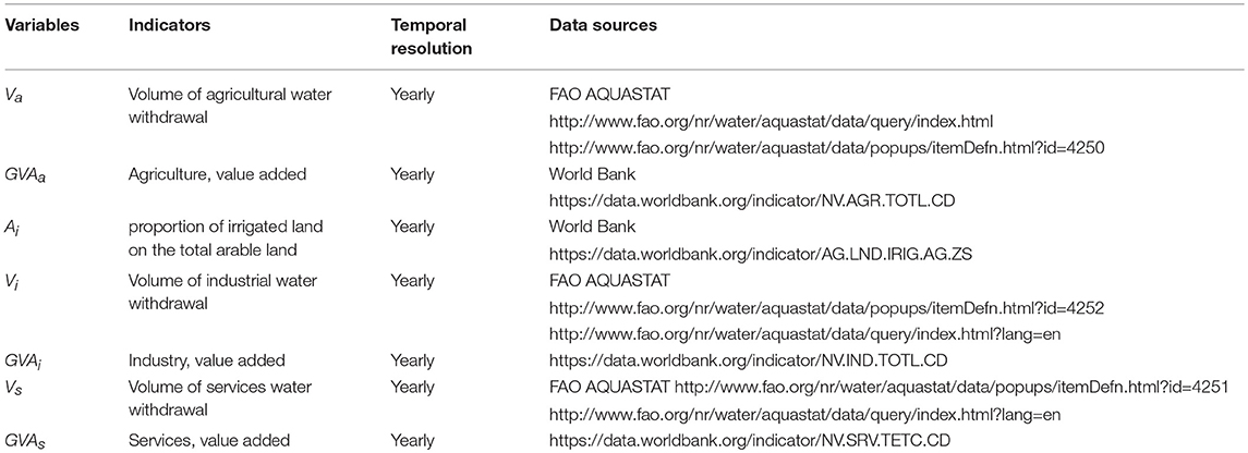
Table 3. Data sources for country level calculation of WUE.

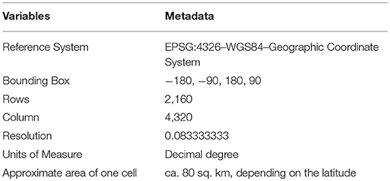
Table 4. Metadata information of developed GIS layers.

Initially, we have calculated country-level WUE for the year 2016, as required by FAO, for comparative purposes. Even if almost all data layers were downloaded at global level, as stated above, we have focused our assessment on South and South-East Asia, by framing maps according to a window with North-East corner longitude 73° latitude 34°N and South-West corner longitude 110° latitude 5°N.

The entire data processing has been conducted in the TerrSet GIS environment, by Clark University (version 18.31) and coded in a single macro file, to allow for easy revisions and updates. Figure 1 presents a flow-chart of the procedure.

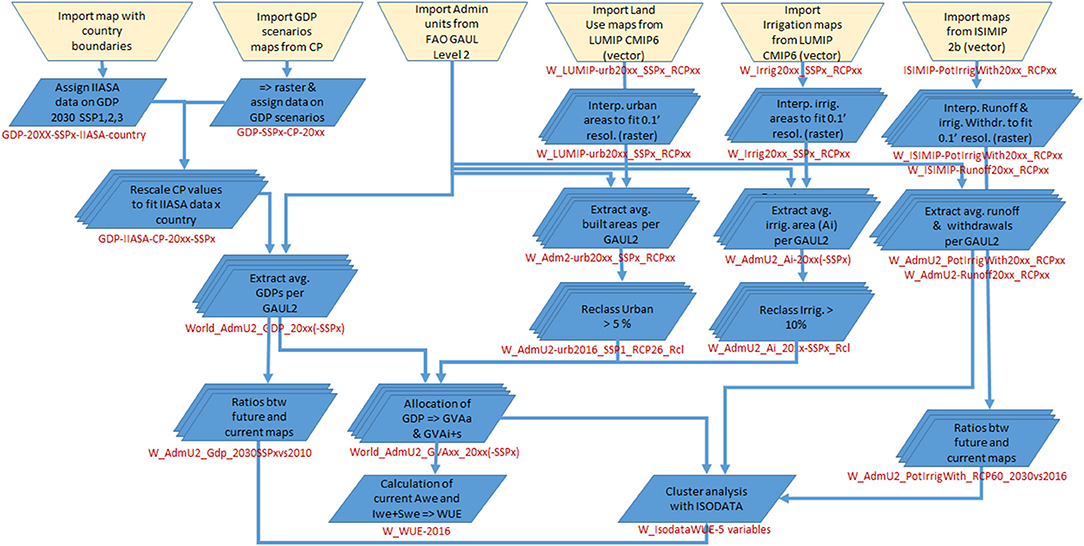
Figure 1. Flow-chart of the proposed approach (file nomenclature in red).

Spatial Analysis of WUE

The gridded estimations of GDP carried out by Murakami and Yamagata (2016) in the Carbon Project¹ were used for building spatially explicit maps of the values of economic activities, going well-beyond country level. Murakami and Yamagata (2016) assessed global population and GDP scenarios in 0.5 × 0.5 degree grids between 1980 and 2100 with an interval of 10 years. For the historical period (1980–2010), the data is estimated by downscaling actual populations and GDPs by country, while for the future (2020–2100) values are estimated by downscaling projected populations and GDPs under three Shared Socioeconomic Pathways (SSP): SSP1; SSP2; and SSP3, by country (source: IIASA SSP database version 1)².

Using the above method, gridded GDP value in 2010 is considered as the most recent available map, while the GDP projection for 2030 (end of Agenda 2030 period) is mapped for three SSPs (SSP1 refers to “Sustainability-Taking the Green Road”, SSP2 indicates “Middle of the Road,” while, SSP3 refers “Regional Rivalry–A Rocky Road”). A series of tests were conducted to verify the coherence between different sources of GDP information (WB, IMF, and IPCC-SSP) and sector GVA's. Eventually, the spatially explicit maps of GDP sum up at the total GVA country values, provided by WB, thus allowing for obtaining comparable results between the country level exercise and the spatial analysis. While future projections fit the values of IIASA.

In order to increase the visibility of the maps we aggregated the cell values (ca. 80 km²) at the level of FAO Global Administrative Unit Layers (GAUL) 2, reported in Figure 2 (source: FAO Geonetwork)³.

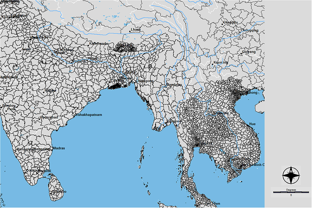
Figure 2. FAO Global Administrative Unit Layer (GAUL) Level 2.

In order to allocate total GDPs per GAUL2 into agriculture as well as industry and service sectors, we have incorporated the land cover map for current and future periods (i.e., 2030) of 3 SSPs in the GIS layer. The land cover maps were collected from the Land Use Model Intercomparison Project (LUMIP) (Lawrence et al., 2016), data set prepared for the Coupled Model Intercomparison Project Phase 6 (CMIP6) (Eyring et al., 2016). In addition to a land cover map, irrigation maps for current and future periods (considering the 3 SSPs) were also imported from LUMIP. The imported land cover and irrigated agriculture maps were used to guide the allocation of GDP, to irrigated areas as the sources of agricultural value added of water withdrawn and built up areas for the allocation of industrial and services value added. By comparing GDP maps with land use and irrigation maps, we distributed total GDP estimations by the Carbon Project into 3 land typologies: (i) GDP of industrial or service origin in those areas with higher GDP and high percentages of built up areas; (ii) GDP of agricultural origin in areas with significant percentage of irrigated agriculture and intermediate GDP values; and (iii) the remaining areas where low GDP values in areas with no significant presence of irrigated agriculture.

For assessing the proportion of agricultural GVA produced by rainfed agriculture (C_r) per GAUL2, using Equation (3), the proportion of irrigated land on total arable land is extracted from LUMIP irrigation area map. Current aggregated figures of water withdrawal for agriculture and other sectors are extracted from recent national statistics shown in Table 3.

An important caveat we would like to stress here is that the data used for this analysis, both the SSP and the LUMIP projections, are result of global scale modeling exercises affected by a certain degree of uncertainty. As stressed in the literature presenting the results of those projects (Lawrence et al., 2016; Riahi et al., 2017), the number of models used for the production of these datasets is relatively limited, and the observed data use for their calibration and validation rather scattered over space and time. Moreover, the future outcomes of current climate change adaptation and mitigation policies, or the lack of effective strategies, are likely to change the socio-economic conditions that have been hypothesized for the scenarios here utilized (Prestele et al., 2016). The uncertainty brought to the analysis presented in this paper by the use of these data is rather difficult, if not impossible, to estimate.

Assessment of Nexus Between Water and Agriculture

Given that the purpose of the work is to make use of freely available spatial information, in order to explore the nexus between water use for economic purposes in general and food production, we acquired the results of the most recent projections of the Inter-Sectoral Impact Model Intercomparison Project (ISIMIP2b) (Frieler et al., 2017).

The rationale behind the approach developed here is that having assessed the current status of economic uses of water, the strategies to be implemented to improve WUE should be tailored to the local situation in terms of: (i) potential for future economic development in general, i.e., GDP changes between future (2030) and current period; (ii) potential for future development of irrigated agriculture, in terms of changes of potential irrigation withdrawal between future (2030) and current period; and (iii) estimated future availability of water resources, using as a proxy the estimated runoff volume. Runoff volume can be considered a good indicator of the surface components of the locally generated blue water resources that, however, is limited in capturing the amount of resources flowing from upstream and fails to account for stocks of groundwater resources.

Depending on current levels of value added generated by water withdrawals and on what emerges from future scenarios (in terms of development, irrigation expansion and water availability), competent administrations can identify promising strategies for the achievement of the SDGs. For example, in areas with relatively low level of current development, but with great future potential, strategies would depend on expected water availability. They could be oriented toward infrastructural investments, in case of high availability of water resources, or toward investments for improving the efficiency per cubic meter of water, when expected availability of water resources is low.

A very preliminary exercise of zoning in support of policy design was thus carried out by using an ISODATA cluster analysis technique (Iterative Self-Organizing Data Analysis Technique), which is a consolidated k-clustering method used for identifying land classes from stacks of multiple images in remote sensing studies (Johnson and Wichern, 2007; Richards, 2013). The map of ISODATA clusters provides a synthesis of multivariate spatial variability of the most important variables characterizing current and future WUE in the region and can be considered as a preliminary support for the identification of a series of different zones characterized by relative internal homogeneity, thus requiring different approaches in terms of policies and measures for the achievement of Target 6.4.

For assessing GDP changes, we calculated the ratio of GDP values between 2030 and current period. Similarly, the ratio of potential irrigation water withdrawal has been calculated between the values of 2030 and those of 2016. Given that runoff estimations varied a lot across the studied area, but showed only limited spatial changes in the comparison between future projection and current estimates, we preferred to use the map of future projections in the ISODATA procedure than calculating the ratio with current values.

We have considered yearly agricultural water withdrawal data for multi-model-mean of four General Circulation Models (GCMs) [GFDL-ESM2M (Donner et al., 2011), HADGEM2-ES ((Bellouin et al., 2011; Collins et al., 2011)), IPSL-CM5A-LR (Dufresne et al., 2013), MIROC5 (Watanabe et al., 2010)] under two climate scenarios (RCP 2.6 and RCP6.0) from global hydrologic model, H08 (Hanasaki et al., 2018). In order to account for inter-annual variability, water withdrawal data are calculated based on 10 years average: current period 2015 represents average yearly value of 2011–2020 and future (2030) value by averaging yearly value of 2026–2035.

Results

Country Level Water Use Efficiency

The current WUE values per country, calculated with the most recent information available in the databases reported in Table 3 is shown in Figure 3.

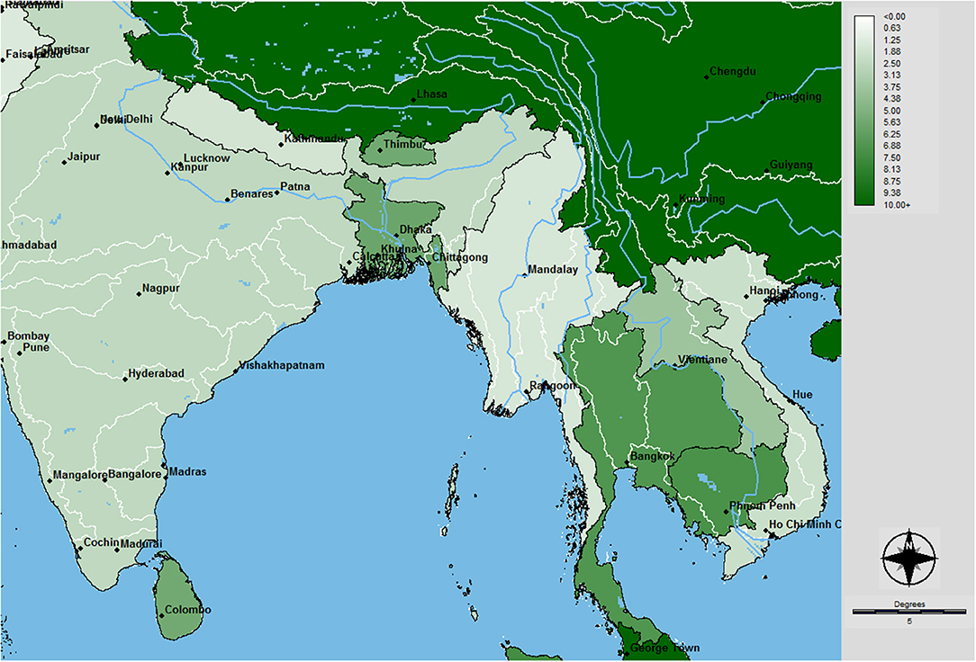
Figure 3. Water use efficiency (US$ m⁻³): current national average values of countries included in the frame of the study area.

The country level results of WUE as shown in Figure 3 are in line with those produced by international organizations (UN-Water, 2018). Only very simplistic comparisons can be derived from the map: e.g., the relatively high value of China, or the relatively lower value of Nepal. Evidently, values averaged at national level are too aggregated and do not present any regional and local variations and hence, there is no information useful for the analysis of the cause-effect links of the phenomena that produced such results, and thus no sound basis for the development of strategies for improving current values to meet Target 6.4, by country or regional governments. Therefore, the assessment of WUE should go beyond country boundaries, with a spatial detail that allows the identification of the combination of environmental and socio-economic drivers, determining the current situations in terms of WUE. Moreover, future projections are needed to compare the current situation with possible future trajectories of those drivers, thus being able to anticipate possible future developments and to design robust policies in view of future scenarios.

Spatial Analysis of WUE

Following the procedure concisely described above, we first mapped GDP values at 0.5° resolution from the Carbon Project as at FAO GAUL 2 level for current period and for three scenarios of SSPs of the future period of 2030. The results of aggregating GDP values at the GAUL 2 level are reported in Figure 4, showing, in general, projected increases in GDP for the studied area, independently from the SSP scenario, but with some differences in the allocation of economic activities moving across the SSPs.

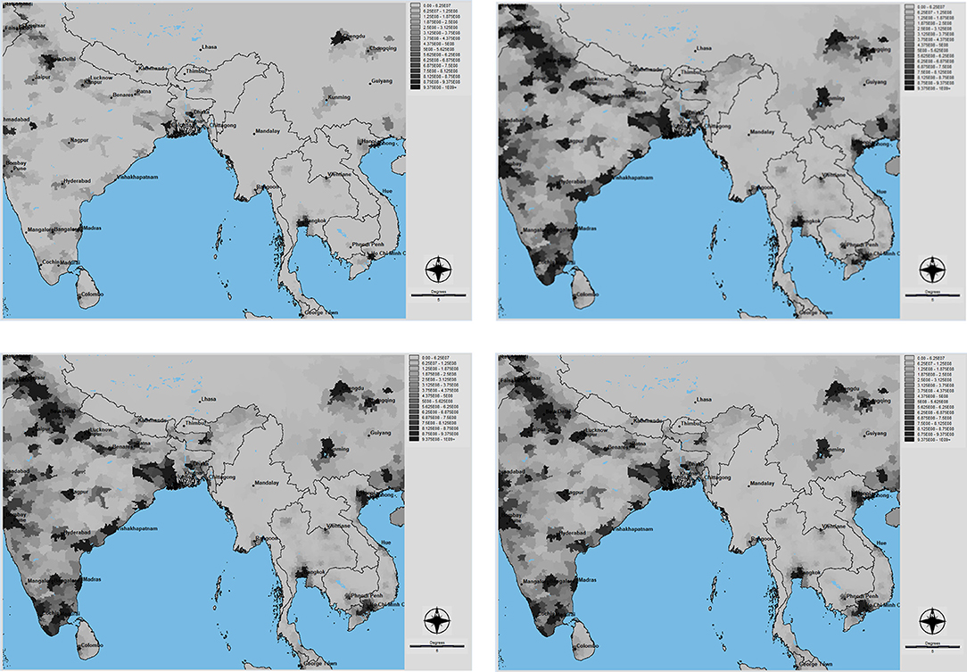
Figure 4. Current GDP (top left) and projected GDP per administrative units (FAO GAUL2) in US$ per pixel (~80 km²): SSP1 (top right) SSP2 (lower left) and SSP3 (lower right).

Considering the most recent statistics on water withdrawals (agricultural, industrial and domestic) and disaggregated GDP into irrigated agriculture and built-up areas as described above, the current value added of water (in US$) at the GAUL2 has been assessed. The spatial allocation of WUE for Southeast Asia is shown in Figure 5. The high value of WUE (represented through deep magenta color in Figure 5A) is shown mainly in built-up areas where industry and urban centers are located, while intermediate levels of water value added are found in irrigated agricultural area (see also Figure 5B,C for more details). By comparing Figure 5 with Figure 3, the potential of accurate spatial analyses clearly emerges. Figure 4 shows all the areas in which current human activities are generating value added from water withdrawals. These are areas where policy interventions to improve WUE required by SDG Target 6.4 should find priority implementation.

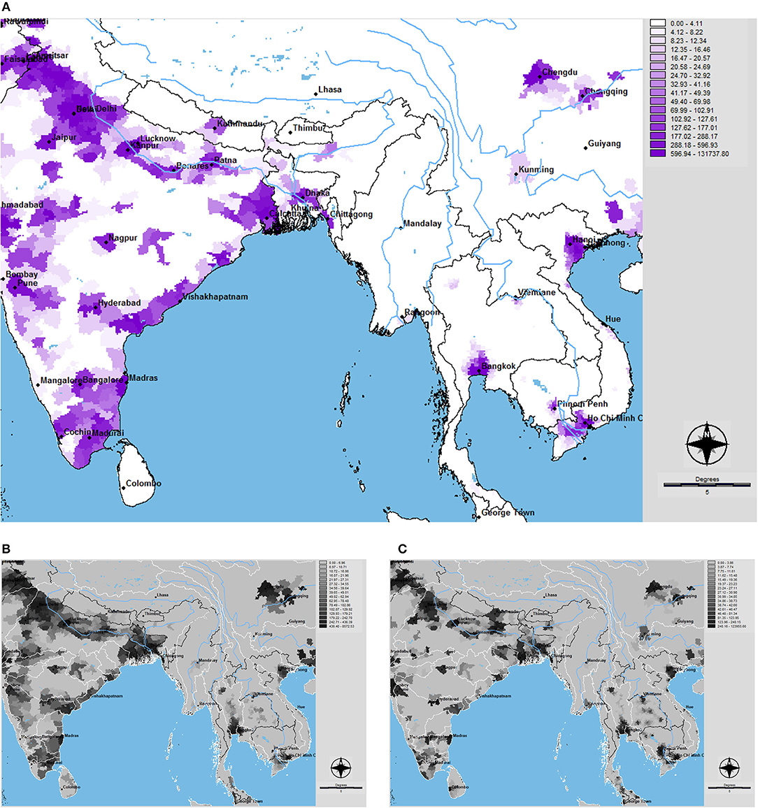
Figure 5. Top (A): Current value added generated by water (in US $) per pixel (~80 km²) at the GAUL 2 level of administrative units; bottom left (B): value added from the agricultural sector; bottom-right (C): value added from industrial and service sectors.

Having identified the priority areas, the need emerges to identify which policies to implement, taking into consideration the relationships among water intensive economic activities and other environmental and socio-economic dynamics. Here, the nexus between food production–and more specifically food produced with irrigated agriculture, and other uses of water is of greater relevance. In terms of value added per unitary volume of water, the primary sector cannot compete with the secondary and tertiary ones, but strategic decisions should be taken at policy level to rule the emerging trade-offs and conflicts and exploit potential synergies, with the aim of maximizing the benefit for society as a whole.

As stated before, the policy options to be implemented will depend on how social and ecological systems will evolve in the future. In this work, we considered future projections of economic growth, the expected development of irrigated agriculture and the changes in water availability as three very important drivers for policy design in water management.

As previously stated, cluster analysis was chosen as a technique to identify areas with similar combination of current and future values of driving variables. By analyzing a stack of 5 images in ISODATA, we produced a map with the identification of typologies of areas that can be used as a preliminary zoning to support the development of water management policies in the region. The five images were current value added for the agricultural sector, the value added of services and industry, future water availability (using estimated runoff volumes as a proxy), the GDP ratio (between 2030 and current period) and the potential irrigation water withdrawal ratio (between 2030 and current period). The procedure was set to obtain 10 clusters showing interesting distinctive average features (see Table 5 and Figure 6 with the histogram of normalized values). The description of each cluster deriving for the different combination of the five independent variables is shown in Table 6, while Figure 7 shows the spatial distribution of the clusters. Indeed, the clusters produced by the ISODATA procedure depend on the specific geographical frame of analysis. With a different frame, but also with different parametrization the results will not be the same. However, the analysis of sensitivity for exploring the effects of variations on ISODATA inputs demonstrated that the main typologies of zones concisely described in Table 6 remain rather stable.

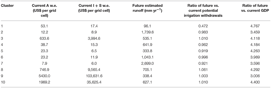
Table 5. Average values of clusters.

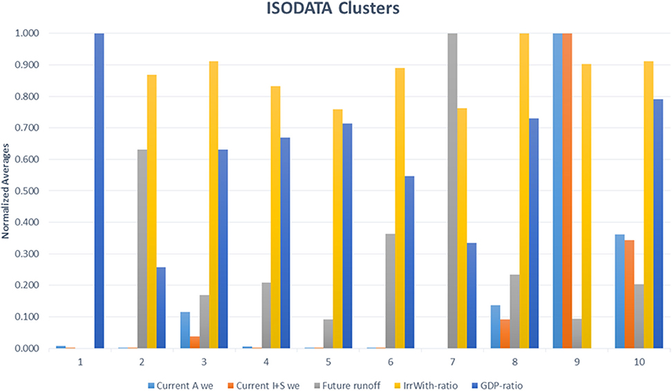
Figure 6. Results of ISODATA classification: normalized average values of the 10 clusters.

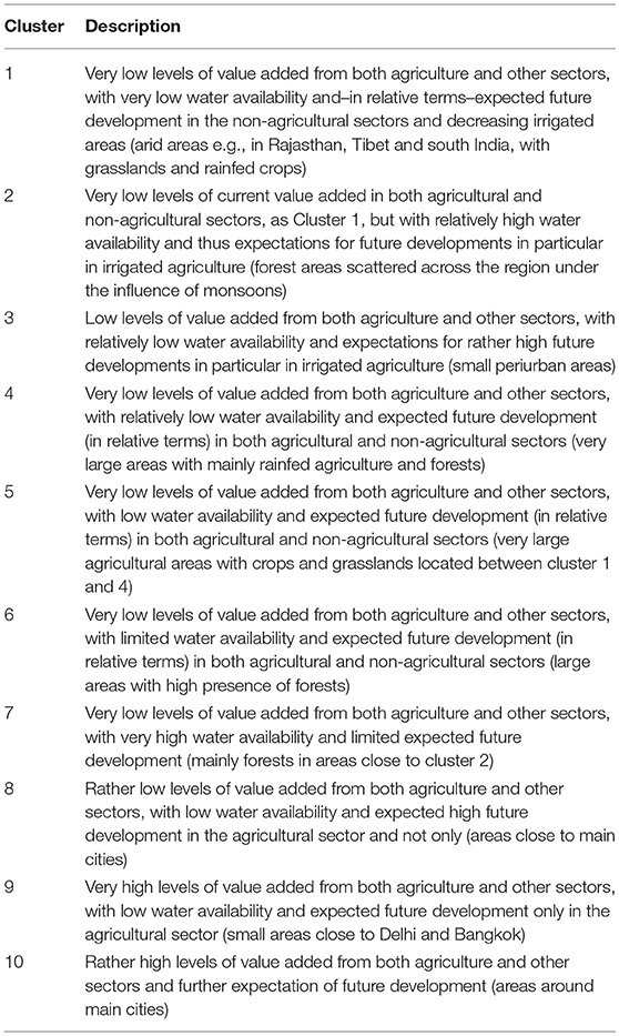
Table 6. Identification of clusters.

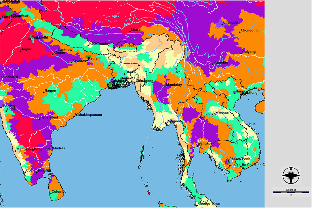
Figure 7. Results of cluster analysis with five variables, to guide the identification of water management policies.

The results of cluster analysis briefly described in Table 6, point out at least three macro-areas that should be subject to different policies. Cluster 2 and 7, are mainly forested and with limited future needs of investments in water infrastructures given the current status and future prospect of availability of water resources and land uses. Cluster 1, 3, 4, 5, 6, 8 are areas of potential future development, where improvements of WUE are to be considered as a priority to avoid conflicts over water resource allocation among different economic sectors. Cluster 3 and 8 are in a peculiar situation, since they are mainly located close to very important urban areas, as are Cluster 9 and 10, where the demand and the potential value added of water are high and so are potential future conflicts for water resource allocation between agriculture and other sectors.

The uncertainty associated with the various input layers should be carefully considered, taking into account the spread of the values of the same variables in various locations. For example, scenario maps of potential irrigation withdrawals vary more in areas of active development, such as the Indo-Gangetic plain, while GDP estimation varies a lot with changing scenarios in built up areas. The robustness of proposed policies will depend on their capabilities to maintain their benefits even with varying future contexts.

Conclusions

Agenda 2030 imposes huge challenges to governments all over the world in their efforts to identify the most effective strategies and implementation measures for achieving the numerous goals and targets. These challenges are particularly strong for those countries with lower resources and more limited data. Considerable efforts have been invested by international institutions and UN agencies for facilitating the identification and access to data sources with global coverage. UN Water launched an Integrated Monitoring Guide for SDG 6 and released a series of step-by-step monitoring guidelines⁴, for monitoring the various indicators, in which data sources at national level are identified. Unfortunately, the quality of available information is often not adequately documented by metadata, thus making an accurate assessment of uncertainty practically impossible as it was in this case. Moreover, the available country statistics presented are referred to different years and time series are very limited, making historical dynamic analyses impossible in vast parts of the world.

In parallel to those efforts focused on national statistics, a wealth of coordinated modeling efforts are in progress to support climate change studies and policy analyses. Here we took advantage of the Land Use Model Intercomparison Project (LUMIP) (Lawrence et al., 2016), set up for the forthcoming Coupled Model Intercomparison Project Phase 6 (CMIP6) (Eyring et al., 2016) and the Inter-Sectoral Impact Model Intercomparison Project (ISIMIP2b) (Frieler et al., 2017). While it is evident that modeling efforts cannot replace data limitations, it seems also evident that such coordinated efforts developed upon shared scenarios and common assumptions represent a great opportunity in particular for less developed countries. In particular, they make freely available state of the art historical simulations and future projections with global coverage, which allows for global, but also regional synoptic analyses across country boundaries (e.g., transboundary river basins) with unprecedented spatial detail.

In this work we attempted the integration of available statistics with those recently released global datasets, considering that the combination of the two can substantially improve monitoring and analyses based only upon country statistics. Very importantly, the use of spatially disaggregated future projections is a prerequisite for moving from SDG monitoring, to policy support for the achievement of the Goals. The identification of effective policies is impossible without having the capability to make projections into the future, but not necessarily developing new models, particularly when the ambition is to explore operational solutions to current and emerging water management issues, at regional and sub-national levels, in areas where national statistical systems are less developed, as in most of developing countries.

Official documents and guidelines ask for country scale assessments, but instead the emphasis should be placed on detailed spatial analysis brought to a level of detail which allows for understanding of the mechanisms behind observed situations and thus also for the design of targeted policies to improve the current status. The first step in policy development consists in the acquisition of the information needed to develop a knowledge base, organized through a long series of indicators, but assessment procedures should go beyond national level aggregation and zoom into sub-national phenomena. Spatially explicitly future scenarios are needed to design sustainable development policies, with the required medium to long term perspectives. The proposed approach goes in that direction, while being still consistent with the approach proposed at country level by the custodian agencies, to allow for both monitoring and reporting the progress toward the meeting of the SDGs with international coordination and for supporting the identification of targeted policy measures needed at local level.

The approach is demonstrated in South and South-East Asia, an area of great relevance in addressing open issues related to sustainable development and the assessment of the indicator 6.4.1 (Change in water use efficiency), which better exemplifies the integration of socio-economic and environmental issues. Moreover, cluster analysis applied to both current estimations and future projections allows a comparison of the current state of the WUE indicator (SDG6) with future prospects of agricultural and non-agricultural development (SDG 2; 8 and others), and changes in water availability (SDG 15). For example, it allows for the identification of territorial ambits to guide tailored water management policies, with consideration of their linkages to other policy contexts, and thus also other SDGs.

Indeed, this work is focused on a single indicator, without explicit assessment of its interlinkages with others, but the calculation of Water Use Efficiency is in fact focused on the analysis of the nexus between water resources and different economic sectors, agriculture and food production in particular. Strong interlinkages are evident with several targets. In particular target 2.4 on sustainable agricultural systems, of which we analyzed the use of water for irrigation, 6.5 for the contribution of efficient water management across sectors to Integrate Water Resources Management (IWRM) policies, and 15.1 focused on the status of freshwater ecosystems. Some of the input data used for the assessment of target 6.4 can be used for the assessment of other indicators, and the flow chart designed for this work can be easily expanded to include the calculation of other indicators.

Although the kind of analysis that we proposed provides concrete support to the policy making, important limitations are still in place and should be clearly discussed. First of all, the use of modeling outputs especially in areas characterized by limited data availability is certainly a huge advantage, but, at the same time, it brings levels of error and uncertainty that are difficult to estimate and are likely to affect the conclusions of the presented and similar analyses. In this work, uncertainty has been dealt with only by means of sensitivity analysis to explore the effects of varying inputs to the final territorial clusters for policy support, obtaining results which showed limited effects on the identification of clusters. Nevertheless, further research efforts are needed to assess the uncertainty levels brought, respectively, by input data and modeling options, in order to provide an accurate estimation of the robustness of the results. Ideally, data uncertainty could be limited by a more detailed monitoring campaign that the custodian agencies should pursue: the first step toward this direction was represented by the identification of a clear set of indicators, but the course taken will surely be costly and hardly free of impediments.

The approach in this paper should be intended to be a procedure for capitalizing on existing information, applicable in different parts of the world, such as South and South-East Asia, selected in this application for the relevance of open issues related to sustainable development, but also for demonstrating the feasibility in regions with strong limitations in data availability. The same procedure (see Figure 1) can be easily applied to the rest of the world, even though accuracies will vary depending on the uncertainties in the input data. Cluster analysis should be carefully reconsidered at global level, for example by revising the number of clusters, in order to obtain meaningful results.

In the near future, this approach will substantially benefit from the continuous flow of new spatial information made available by the intercomparison modeling exercises mentioned above and by improved statistics. Even more, the zoning proposed here could benefit from ad-hoc integrated modeling exercises, but that would increase time and financial resources needed by orders of magnitude.

Data Availability Statement

The datasets utilized as inputs for this study can be found in the repositories and links identified in the article above (see Table 3, in particular). Intermediate and final results, including data sets, maps and the macro file will be made available by the authors to any qualified researcher.

Author Contributions

CG designed the methodological framework and conducted GIS analyses. FF and AG contributed to the development of the methodology and collected raw data. The three authors jointly wrote the article.

Conflict of Interest Statement

The authors declare that the research was conducted in the absence of any commercial or financial relationships that could be construed as a potential conflict of interest.

Acknowledgments

AG is financially supported by the cluster of excellence, The Future Ocean, funded by the German Research Foundation, whose support is gratefully acknowledged.

Footnotes

References

Allen, C., Nejdawi, R., El-Baba, J., Hamati, K., Metternicht, G., and Wiedmann, T. (2017). Indicator-based assessments of progress towards the sustainable development goals (SDGs): a case study from the Arab region. Sustain. Sci. 12, 975–989. doi: 10.1007/s11625-017-0437-1
Bellouin, N., Collins, W. J., Culverwell, I. D., Halloran, P. R., Hardiman, S. C., Hinton, T. J., et al. (2011). The HadGEM2 family of met office unified model climate configurations. Geosci. Model Dev. 4, 723–757. doi: 10.5194/gmd-4-723-2011
Collins, W. J., Bellouin, N., Doutriaux-Boucher, M., Gedney, N., Halloran, P., Hinton, T., et al. (2011). Development and evaluation of an earth-system model – HadGEM2. Geosci. Model Dev. 4, 1051–1075. doi: 10.5194/gmd-4-1051-2011
Donner, L. J., Wyman, B. L., Hemler, R. S., Horowitz, L. W., Ming, Y., Zhao, M., et al. (2011). The dynamical core, physical parameterizations, and basic simulation characteristics of the atmospheric component AM3 of the GFDL global coupled model CM3. J. Clim. 24, 3484–3519. doi: 10.1175/2011JCLI3955.1
Dufresne, J. L., Foujols, M. A., Denvil, S., Caubel, A., Marti, O., Aumont, O., et al. (2013). Climate change projections using the IPSL-CM5 earth system model: from CMIP3 to CMIP5. Clim. Dyn. 40, 2123–2165. doi: 10.1007/s00382-012-1636-1
Eyring, V., Bony, S., Meehl, G. A., Senior, C. A., Stevens, B., Stouffer, R. J., et al. (2016). Overview of the coupled model intercomparison project phase 6 (CMIP6) experimental design and organization. Geosci. Model Dev. 9, 1937–1958. doi: 10.5194/gmd-9-1937-2016
FAO (2017). Integrated Monitoring Guide for SDG 6. Step-by-step monitoring methodology for indicator 6.4.1 on water-use efficiency. Version 2017-03-10.
Farinosi, F., Giupponi, C., Reynaud, A., Ceccherini, G., Carmona-Moreno, C., De Roo, A., et al. (2018). An innovative approach to the assessment of hydro-political risk: a spatially explicit, data driven indicator of hydro-political issues. Glob. Environ. Change 52, 286–313. doi: 10.1016/j.gloenvcha.2018.07.001
Frieler, K., Lange, S., Piontek, F., Reyer, C. P. O., Schewe, J., Warszawski, L., et al. (2017). Assessing the impacts of 1.5°C global warming – simulation protocol of the Inter-Sectoral Impact Model Intercomparison Project (ISIMIP2b). Geosci. Model Dev. 10, 4321–4345. doi: 10.5194/gmd-10-4321-2017
Gain, A. K., Benson, D., Rahman, R., Datta, D. K., and Rouillard, J. J. (2017a). Tidal river management in the south west Ganges-Brahmaputra delta in Bangladesh: moving towards a transdisciplinary approach? Environ. Sci. Policy 75, 111–120. doi: 10.1016/j.envsci.2017.05.020
Gain, A. K., Giupponi, C., and Benson, D. (2015). The water–energy–food (WEF) security nexus: the policy perspective of Bangladesh. Water Int. 40, 895–910. doi: 10.1080/02508060.2015.1087616
Gain, A. K., Giupponi, C., and Wada, Y. (2016). Measuring global water security towards sustainable development goals. Environ. Res. Lett. 11:124015. doi: 10.1088/1748-9326/11/12/124015
Gain, K. A., Mondal, S. M., and Rahman, R. (2017b). From flood control to water management: a journey of bangladesh towards integrated water resources management. Water 9:1. doi: 10.3390/w9010055
Giupponi, C., and Gain, A. K. (2017). Integrated spatial assessment of the water, energy and food dimensions of the sustainable development goals. Reg. Environ. Change 17, 1881–1893. doi: 10.1007/s10113-016-0998-z
Giupponi, C., Giove, S., and Giannini, V. (2013). A dynamic assessment tool for exploring and communicating vulnerability to floods and climate change. Environ. Model. Softw. 44, 136–147. doi: 10.1016/j.envsoft.2012.05.004
Hák, T., Janoušková, S., and Moldan, B. (2016). Sustainable development goals: a need for relevant indicators. Ecol. Indicat. 60, 565–573. doi: 10.1016/j.ecolind.2015.08.003
Hanasaki, N., Yoshikawa, S., Pokhrel, Y., and Kanae, S. (2018). A global hydrological simulation to specify the sources of water used by humans. Hydrol. Earth Syst. Sci. 22, 789–817. doi: 10.5194/hess-22-789-2018
Johnson, R. A., and Wichern, D. W. (2007). Applied Multivariate Statistical Analysis. Upper Saddle River, NJ: Pearson Education, Inc.
Lawrence, D. M., Hurtt, G. C., Arneth, A., Brovkin, V., Calvin, K. V., Jones, A. D., et al. (2016). The land use model intercomparison project (LUMIP) contribution to CMIP6: rationale and experimental design. Geosci. Model Dev. 9, 2973–2998. doi: 10.5194/gmd-9-2973-2016
Le Blanc, D. (2015). Towards integration at last? the sustainable development goals as a network of targets. Sustain Dev. 23, 176–187. doi: 10.1002/sd.1582
Liu, J., Hull, V., Godfray, H. C. J., Tilman, D., Gleick, P., Hoff, H., et al. (2018). Nexus approaches to global sustainable development. Nat. Sustain. 1, 466–476. doi: 10.1038/s41893-018-0135-8
Liu, J., Yang, H., Cudennec, C., Gain, A. K., Hoff, H., Lawford, R., et al. (2017). Challenges in operationalizing the water–energy–food nexus. Hydrol. Sci. J. 62, 1714–1720. doi: 10.1080/02626667.2017.1353695
Murakami, D., and Yamagata, Y. (2016). Estimation of Gridded Population and GDP Scenarios with Spatially Explicit Statistical Downscaling. ArXiv 1610.09041.
Neely, C., Bourne, M., Chesterman, S., Kouplevatskaya-Buttoud, I., Bojic, D., and Vallée, D. (2017). Implementing 2030 Agenda for Food and Agriculture: Accelerating Impact through Cross-Sectoral Coordination at the Country Level. Rome: Food and Agriculture Organization of the United Nations.
Obersteiner, M., Walsh, B., Frank, S., Havlík, P., Cantele, M., Liu, J., et al. (2016). Assessing the land resource–food price nexus of the sustainable development goals. Sci. Adv. 2:e1501499. doi: 10.1126/sciadv.1501499
Prestele, R., Alexander, P., Rounsevell, M. D. A., Arneth, A., Calvin, K., Doelman, J., et al. (2016). Hotspots of uncertainty in land-use and land-cover change projections: a global-scale model comparison. Glob. Change Biol. 22, 3967–3983. doi: 10.1111/gcb.13337
Reyers, B., Stafford-Smith, M., Erb, K. H., Scholes, R. J., and Selomane, O. (2017). Essential variables help to focus sustainable development goals monitoring. Curr. Opin. Environ. Sustain. 26–27, 97–105. doi: 10.1016/j.cosust.2017.05.003
Riahi, K., van Vuuren, D. P., Kriegler, E., Edmonds, J., O'Neill, B. C., Fujimori, S., et al. (2017). The shared socioeconomic pathways and their energy, land use, and greenhouse gas emissions implications: an overview. Glob. Environ. Change 42, 153–168. doi: 10.1016/j.gloenvcha.2016.05.009
Roy, K., Gain, A. K., Mallick, B., and Vogt, J. (2017). Social, hydro-ecological and climatic change in the southwest coastal region of Bangladesh. Regional Environ. Change 17, 1895–1906. doi: 10.1007/s10113-017-1158-9
Schmidt-Traub, G., Kroll, C., Teksoz, K., Durand-Delacre, D., and Sachs, J. D. (2017). National baselines for the sustainable development goals assessed in the SDG index and dashboards. Nat. Geosci. 10, 547–555. doi: 10.1038/ngeo2985
UN (2015). Transforming our World: 2030 Agenda for Sustainable Development. Res. A/70/L.1. New York, NY: United Nations.
UN (2017). Revised List of Global Sustainable Development Goal indicators. New York, NY: United Nations.
Unver, O., Bhaduri, A., and Hoogeveen, J. (2017). Water-use efficiency and productivity improvements towards a sustainable pathway for meeting future water demand. Water Security 1, 21–27. doi: 10.1016/j.wasec.2017.05.001
UN-Water (2016). Water and Sanitation Interlinkages Across the 2030 Agenda for Sustainable Development. Geneva: UN-Water.
UN-Water (2017a). Integrated Monitoring Guide for Sustainable Development Goal 6 on Water and Sanitation: Good practices for Country Monitoring Systems. Geneva: UN-Water.
UN-Water (2017b). Integrated Monitoring Guide for Sustainable Development Goal 6 on Water and Sanitation: Targets and Global Indicators. Geneva, UN-Water.
UN-Water (2018). Sustainable Development Goal 6 Synthesis Report on Water and Sanitation. Geneva: UN-Water.
Vanham, D., Hoekstra, A. Y., Wada, Y., Bouraoui, F., de Roo, A., Mekonnen, M. M., et al. (2018). Physical water scarcity metrics for monitoring progress towards SDG target 6.4: an evaluation of indicator 6.4.2 “Level of water stress”. Sci. Total Environ. 613–614, 218–232. doi: 10.1016/j.scitotenv.2017.09.056
Watanabe, M., Suzuki, T., O'ishi, R., Komuro, Y., Watanabe, S., Emori, S., et al. (2010). Improved climate simulation by MIROC5: mean states, variability, and climate sensitivity. J. Clim. 23, 6312–6335. doi: 10.1175/2010JCLI3679.1
Keywords: sustainable development goals, water use efficiency, spatial assessment, ISODATA, policy support
Citation: Giupponi C, Gain AK and Farinosi F (2018) Spatial Assessment of Water Use Efficiency (SDG Indicator 6.4.1) for Regional Policy Support. Front. Environ. Sci. 6:141. doi: 10.3389/fenvs.2018.00141
Received: 25 June 2018; Accepted: 05 November 2018;
Published: 22 November 2018.
Edited by:
Richard George Lawford, Morgan State University, United StatesReviewed by:
Sushel Unninayar, Morgan State University, United StatesArgyro Kavvada, Booz Allen Hamilton, United States
Olcay Unver, Food and Agriculture Organization delle Nazioni Unite, Italy
Copyright © 2018 Giupponi, Gain and Farinosi. This is an open-access article distributed under the terms of the Creative Commons Attribution License (CC BY). The use, distribution or reproduction in other forums is permitted, provided the original author(s) and the copyright owner(s) are credited and that the original publication in this journal is cited, in accordance with accepted academic practice. No use, distribution or reproduction is permitted which does not comply with these terms.
*Correspondence: Carlo Giupponi, cgiupponi@unive.it