Introduction

In the last two decades about 100 automatic weather stations (AWSs) have been deployed in Antarctica (e.g. United States Antarctica Program (USAP),Reference Stearns and WendlerStearns and Wendler, 1988). Considering how vast the continent is, the number of observations is still limited. The use of these stations is a relatively cheap and easy way of increasing the number of measurements. An AWS is designed to work for long periods without being serviced and can therefore operate in remote areas and in harsh weather conditions. The AWS data have been used to study meteorological processes close to the surface and climatological conditions in several regions of Antarctica (e.g. Reference Allison, Wendler and RadokAllison and others, 1993; Reference Bintanja, Jonsson and KnapBintanja and others, 1997).

This paper describes the annual cycle of meteorological variables and the surface energy fluxes over Berkner Island, Filchner-Ronne Ice Shelf, Antarctica. Several studies have been carried out on the ice cap of Berkner Island within the framework of the Filchner-Ronne Ice Shelf Programme (FRISP), a research programme of the Alfred Wegener Institute for Polar and Marine Research (AWI), Bremerhaven, Germany. These range from short-pulse echo sounding to ice-core drillings and meteorological measurements (Reference Oerter and OerterOerter, 1995). In February 1995 the Institute for Marine and Atmospheric Research Utrecht (IMAU) deployed an AWS on the south dome of the island, with the aim of providing insight into the meteorological conditions on the island to help with the interpretation of the ice-core analysis.

The station has provided us with a fairly complete 3 year meteorological dataset, which is described here and used to determine the surface energy fluxes. This study proves that it is feasible to derive a fairly accurate estimate of the surface energy balance from relatively simple meteorological measurements made by an AWS. This has the advantage that estimates of the surface energy budgets can be made over longer periods at remote places.

Location and Experimental Set-Up

Berkner Island is a large island completely covered by ice in the Filchner-Ronne Ice Shelf, south of the Weddell Sea (Fig. 1). The AWS measurements were carried out on Thyssen Hohe, the south dome of Berkner Island (79.57° S, 45.78° W; 886 m a.s.l.). Observations started on 12 February 1995. The station samples every 6 min, calculates hourly average data, transmits these data using an Argos transmitter and also stores the data locally. It is designed to work for approximately 3 years without being serviced. The results reported in this paper are based on an almost 3 year meteorological dataset (12 February 1995 to 31 December 1997).

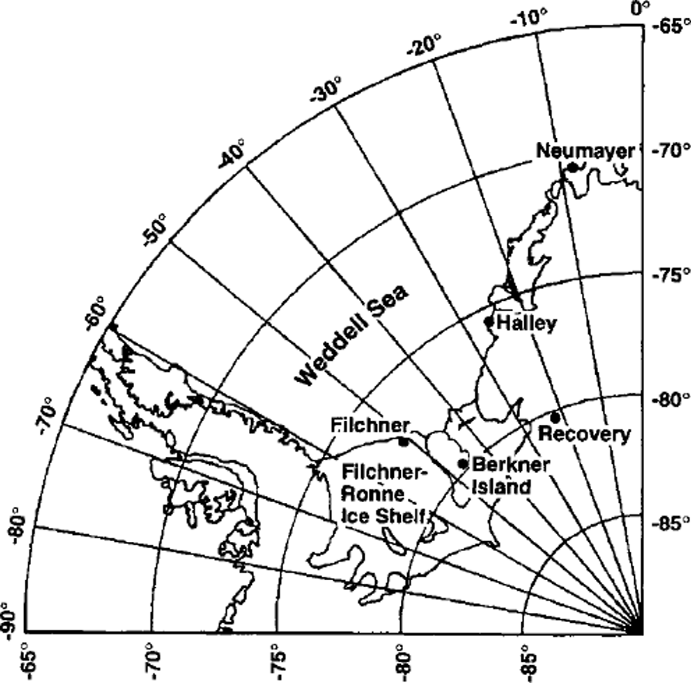
Fig. 1. Location of the weather stations in the Filchner-Ronne Ice Shelf area.

The station consists of a vertical mast placed on a four-legged frame. Near the top of the mast, a horizontal bar is attached on which the air-temperature, wind-speed, wind-direction, instrument-height and shortwave-incoming-radiation sensors are mounted. The AWS also measures snow temperature at two depths (initially 0.1 and 1.0 m) and air pressure (mounted inside the electronics box). The instrument height is a measure of the snow height and is monitored by the station using a sonic altimeter. The AWS is situated in an accumulation zone, so the instrument height is not constant over time. The initial height was 2.95 m.

The accuracy of the sensors was tested in an intercomparison experiment in The Netherlands and near the South Pole before the station was placed on Berkner Island. The sensors are not ventilated, which affects the accuracy, particularly, of the temperature sensor. Problems with the data transmission led to gaps in the dataset of a few hours to a few days. About 8% of the data are lost in this way. The most serious problems were caused by rime forming on the sensors. This causes the wind-speed and wind-direction sensors to seize, and shields the instrument-height and shortwave-radiation sensors. As a result, data from these sensors are unreliable between 4 April 1995 and 30 October 1995 and for some briefer periods.

We will compare the meteorological conditions on Berkner Island with the conditions at Halley station and at Recovery Glacier AWS. Halley station is a permanently occupied British base on the Brunt Ice Shelf, which is located in the southeastern part of the Weddell Sea region (75.45° S, 26.4° W; 37ma.s.l.). Meteorological measurements at this station started in 1956. Recovery AWS was placed on Recovery Glacier, situated south of the Shackleton Range, in 1994 (80.8° S, 22.3° W; 1220 m a.s.l.). Only data for 1995 are available from this AWS.

Meteorological Conditions

Figure 2 shows the temporal variations in the daily mean values of air temperature, wind speed, air pressure and instrument height during the measuring period. The AWS records show that the near-surface meteorological conditions on the south dome of Berkner Island are very variable. Besides the seasonal variability, large variations occur on time-scales of days and weeks. Because the station was placed on a dome, the near-surface climate is probably mainly influenced by synoptic-scale weather systems and relatively unaffected by katabatic flow, for which a slope in the terrain would be necessary.

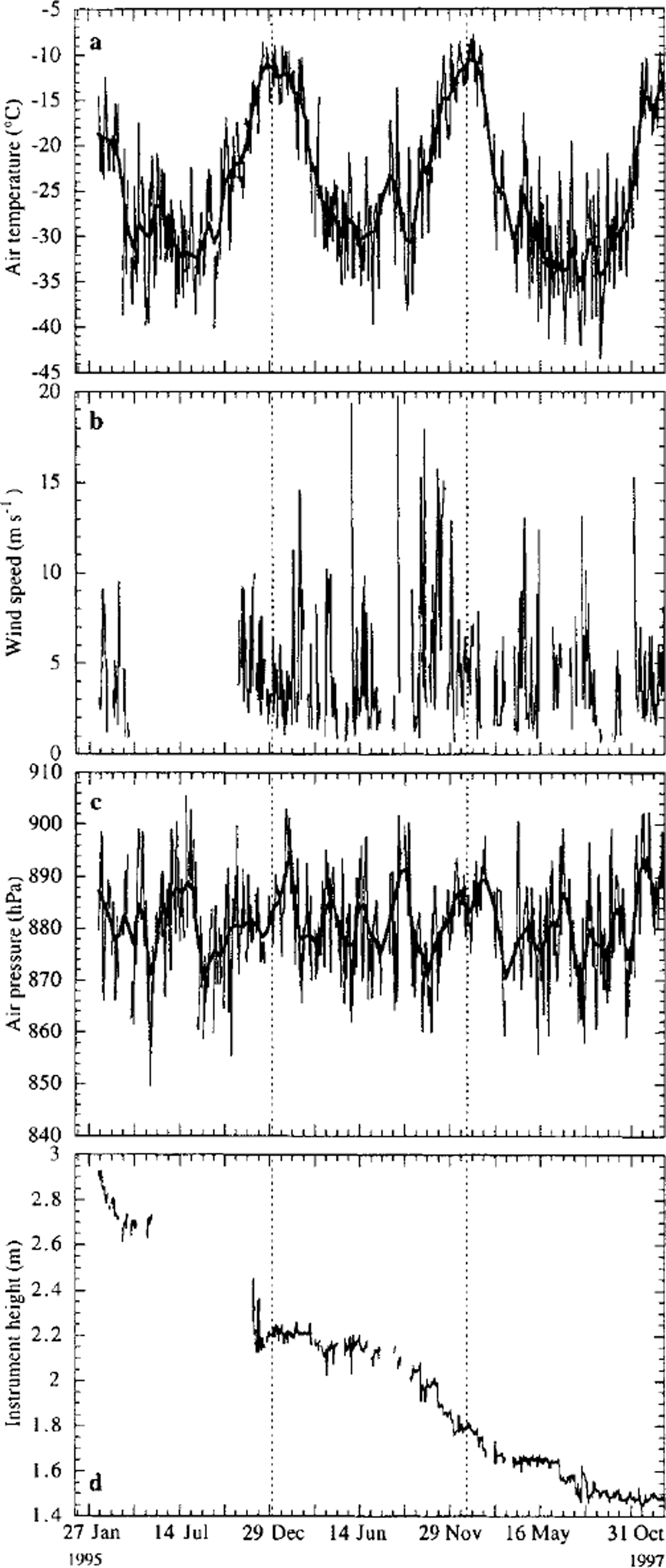
Fig. 2. Variation in the daily mean values of air temperature (a), wind speed (b), air pressure (c) and instrument height ( d) over the entire measuring period. The thick line is a smoothed curve.

The absence of a predominant katabatic flow is shown in the wind-speed (Fig. 2) and wind-direction results. The wind speed is quite variable throughout the measuring period. Although large gaps are present, no significant annual variation is observed. Daily mean values vary between 0 and 20 ms⁻¹, and wind-speed maxima (6 min means) can reach 50 ms⁻¹. The annual mean wind speed is about 4.5 ms⁻¹, which is low compared to other Antarctic stations. The annual mean wind speed for Halley, Recovery and Dumont d’Urville is 6.7, 5.5 and 9.4 ms⁻¹ (Reference King and TurnerKing and Turner, 1997), respectively. These stations are all affected by katabatic flow. Dome C, a station on a dome not affected by katabatic flow, observes an annual mean wind speed of 2.9 ms⁻¹ (Reference Wendler and KodamaWendler and Kodama, 1984).

In general, the wind direction is variable, with a weak preference for directions of around 10° from north. Variability of the wind direction is expressed in the directional constancy, which is the ratio of the magnitude of the vector mean wind speed to the scalar mean. A high directional constancy implies that the wind prefers a particular direction. The directional constancy based on hourly means for Berkner Island is 0.38, which, for Antarctic conditions, can be considered low. Halley has a directional constancy of 0.59. Recovery and Dumont d’Urville each have a high directional constancy, of 0.90 and 0.91, respectively.

The summer on Berkner Island is short and peaked, temperatures during the summer remaining below 0°C. The highest recorded hourly mean temperature was -3.1°G (28 January 1996), so no significant melt is expected. The lowest recorded temperature was -46.0°C (4 September 1997). During winter, temperature fluctuations of 20°C or more occur within a few days. The absence of melt implies that mass loss is caused entirely by wind erosion and/ or sublimation. Figure 2 shows that the height of the sensor bar decreases by 1.45 m over the measuring period. Snow-pit measurements 5 km from the AWS yield a mean near-surface snow density of 368.2 kg m⁻³ (Reference Oerter and OerterOerter, 1995), resulting in an annual accumulation of about 180 mm w e. a–1. Results from anicecore drilled near the snow pit.reveal an annual mean accumulation of 170 mm we. a⁻¹, based on about 20 years’ accumulation (Reference WagenbachWagenbach and others, 1994). The interannual variability is large. In 1995, 0.73 m snow accumulated near the AWS, comparedto0.40 and0.32 min 1996 and 1997, respectively.

Table 1 shows the annual mean values and extremes (based on daily averaged values) of the meteorological parameters for the measuring period. The table also summarises the annual mean values for Halley station (based on monthly averaged values) and for Recovery AWS (based on daily averaged values). Note that for Berkner Island, January is missing for the year 1995. To obtain a mean value over a complete year, values for January 1996 are substituted for those in January 1995. Furthermore, 63% of the wind-speed and wind-direction data were lost through rime forming in 1995. The calculated annual mean values are based on the remaining 37%. For Recovery AWS, only data for 1995 were available.

Table 1. Annual mean and extreme values of the meteorological data for Berkner Island AWS (based on daily averaged values), Halley station (based on monthly averaged values) and Recovery AWS (based on daily averaged values). Plus the long-term annual mean for Halley station (Reference King and TurnerKing and Turner, 1997)

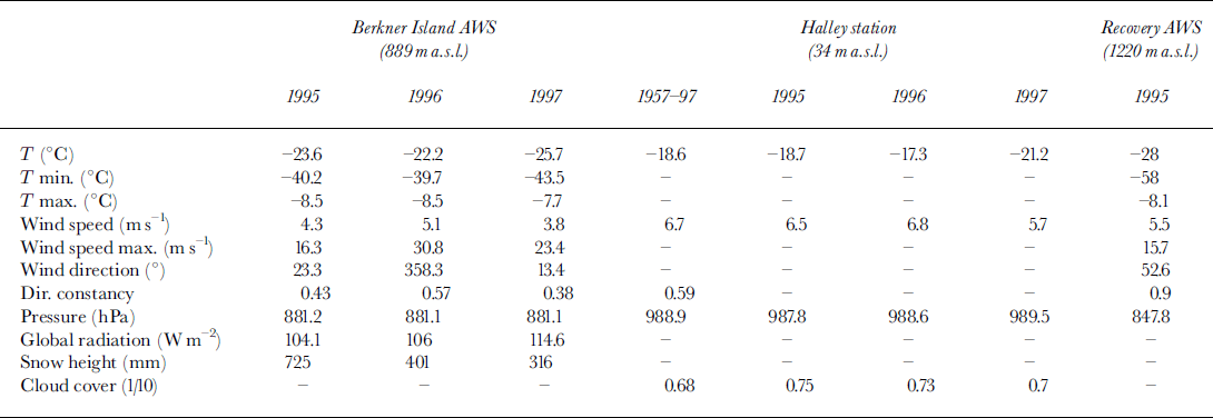
The annual mean temperature for Berkner Island over the measurement period is about -24°C. The 10 m snow temperature, a measure of the annual mean surface temperature, is -26.4°G. For both Halley station and Berkner Island, 1996 was a warm year with high wind speeds. The temperature at Halley and the AWS site was about 1.5°G warmer than the long-term mean. The directional constancy for Berkner Island was also high. The year 1997, on the other hand, was very cold for both stations. The temperature for the AWS was about 2°C lower than the annual mean over the 3 year period, mainly because of the low winter temperatures. The temperature for Halley was almost 3°C lower than the long-term mean. Other meteorological quantities also show extreme values for 1997 compared to the long-term mean. For instance, the wind speed for both stations is low, the shortwave incoming radiation for Berkner Island is high and the changes in snow height are small. Furthermore, the mean cloud cover measured near Halley is low compared to the other two years. Although the two stations are about 700 km apart, the high value of incoming shortwave radiation, the low mean temperature and the low mean cloud cover indicate lower cyclonic activity in 1997. This is reflected in the higher annual mean pressure for Halley station and the higher pressure in February, November and December 1997 for Berkner Island (Fig. 2c).

Surface Energy Balance: Model Description and Assumptions

The model used to compute surface energy fluxes is described in Reference Greuell and KonzelmannGreuell and Konzelmann (1994). They used the model to calculate the surface energy balance for the Swiss Federal Institute of Technology (ETH) camp location, West Greenland. We adjusted the model to suit the situation on Berkner Island. The model will be described briefly to illustrate the adjustments that were made.

The model consists of an atmospheric part and a firn part. No adjustments were made in the firn part of the model. In the firn part the model calculates the temperature and density on a grid extending vertically from the surface into a 25 m thick snow layer. The distance between the gridpoints of the snow model changes exponentially from 50 mm at the surface to 3 m at a depth of 25 m. On this grid the thermodynamic energy equation is solved:

(1)

where p is the density, c_pi is the heat capacity of ice, K is the effective conductivity, ∂Qt_/∂z is the absorption of energy from the atmosphere, M is the melt rate, F is the freezing rate and L_M is the latent heat of fusion. In the uppermost layer of the model, Q_t is the sum of the radiative and turbulent fluxes. In the following layers Q_t is the shortwave radiation penetration. K is a function of the density and is calculated using Von Dusen’s equation:

(2)

Densification of the snowpack is possible through internal melting and/or refreezing. Furthermore, empirical relations developed by Reference Herron and LangwayHerron and Langway (1980) describe settling and packing of the snowpack.

In the atmospheric part of the model, the radiative and turbulent fluxes are calculated. Generally, if there is no melt, the surface energy balance is written as (fluxes towards the surface are positive):

(3)

where S is the net shortwave radiative flux (incoming minus reflected), L is the net longwave radiative flux (incoming minus emitted), H and LE are the turbulent fluxes of sensible and latent heat, respectively, and G is the subsurface energy flux. The model is forced by five meteorological quantities, namely, air temperature, wind speed, air pressure, incoming shortwave radiation and snow-height changes. The AWS does not measure humidity, and therefore relative humidity was set to a constant value of 70% based on Filchner station measurements.

The snow-height changes were derived from the instrument-height measurements and influence the size and density of the uppermost grid layer. In the case presented here, the net shortwave radiation is derived from incident radiation measurements and using an albedo of 0.8 (Reference Bintanja and van den BroekeBintanja and Van den Broeke, 1995). The longwave incoming radiation is calculated using the parameterisation of Reference KingKing (1996), which is derived from monthly mean values of incoming longwave radiation and temperature at four Antarctic stations:

(4)

where T _a is the screen-level temperature in K. The temperature measurements are corrected to give T _a. The longwave outgoing radiation is calculated using the Stefan-Boltzmann law with an emissivity of 1, and the surface temperature (T ₀) derived from the firn part of the model.

The fluxes of sensible and latent heat are calculated using Monin-Obukhov similarity theory. In the atmospheric surface layer the mean gradients of wind speed (u), potential temperature (9) and specific humidity (q) are assumed to be related to the corresponding fluxes according to the flux-profile relations:

(5a)

(5b)

(5c)

where κ is the von Karman constant (≈ 0.4), z is the height above the surface, u* is the friction velocity, 6_, is the turbulent temperature scale, q_* is the turbulent humidity scale, ξ is a non-dimensional length scale (= z/ L_mo in which L_mo is the Monin-Obukhov length scale) and ϕ_m and φh are the non-dimensional stability functions for momentum (m) and heat (h), respectively. The non-dimensional stability function for moisture is assumed to be equal to φh. In unstable conditions (£ < 0) the expressions for ϕ of Reference DyerDyer (1974) and Reference HogstromHogstrom (1988) are used. In stable conditions (£ > 0) the expressions for ϕ of Reference DuynkerkeDuynkerke (1991) are used. Assuming a constant flux layer, the flux-profile relations can be integrated analytically between two heights. The surface-roughness length of momentum (z₀) is empirically derived and assumed to be 1.0 × KT⁴m (Reference King and TurnerKing and Turner, 1997). The surface-roughness lengths of heat (z_h) and moisture (z_q) are calculated using the method described by Reference AndreasAndreas (1987). At z₀ the wind speed is zero and the specific humidity becomes the ice-saturation value for T₀. Knowing the surface-roughness lengths, the humidity and the wind speed and temperature at two levels, it is possible to compute u‡, 6, and q* using an iterative method. The turbulent fluxes of sensible (H) and latent (LE) heat can then be calculated with:

(6a)

(6b)

where p_&amp; is the air density, c_pa is the heat capacity of air at constant pressure and L_s is the latent heat of sublimation.

Surface Energy Balance: Results

In Figure 3 the modelled and measured subsurface temperature at two depths are shown for the entire measurement period. The sensor depths were 0.1 and 1.0 m initially, and slowly increased due to accumulation. The model is able to simulate the measurements but underestimates the temperature at both levels. During summer the differences are largest but generally remain smaller than 4°C. At larger depth the differences diminish. The mean difference between the modelled and measured temperature is –1.0°C at the 0.1 m level and –0.8°C at the 1.0 m level. Reference Greuell and KonzelmannGreuell and Konzelmann (1994) also found differences of this magnitude between their modelled and measured subsurface temperature on Greenland. They attributed the differences to a thin layer of snow over an ice surface, which was not represented in the model, or to a deficiency in the simulation of internal melting. In our case, however, the snow layer is thick enough and no internal melting takes place.

Fig 3. Daily mean values for the simulated (solid line) and measured (dashed line) snow temperatures at two depths over the entire measurement period. Also shown is the difference between the simulated and measured temperatures.

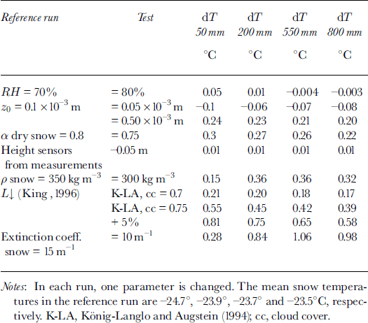
A problem in our case is the fact that we have no direct measurements of the longwave radiation fluxes or measurements of the turbulent fluxes. This means that parameterisations are needed to calculate these fluxes. Table 2 shows the sensitivity of the snow temperature to changes in the model parameters and measurements. The table shows that the temperatures are sensitive to changes in the longwave incoming flux and the extinction coefficient of shortwave radiation penetration in snow. The model is less sensitive to changes in surface roughness, relative humidity or surface albedo. The influence of the changes is largest at shallow depth and diminishes with increasing depth. More sophisticated routines calculating the extinction coefficient are available (Reference Brandt and WarrenBrandt and Warren, 1993) but require the solar radiation to be treated in small wavelength bands, which is not the case here. Considering the limited number of variables measured and the large number of assumptions made, the simulation can be regarded as reasonably good. Also, the changes introduced to the reference run are rather extreme.

Table 2. Changes in mean snow temperatures at 50, 200, 550 and 800 mm depth with a change in model parameters or measurements with regard to the reference run

Accepting the calculated energy fluxes in the reference run, Figure 4 shows the monthly mean surface energy fluxes for the complete period. To obtain estimates throughout winter 1995, the long-term mean wind speed is used and the sensor height is linearly interpolated. During winter the net radiation flux (R) is fully determined by the net longwave radiation flux (L). R is negative, upward-directed (-10 to -20 W m⁻²), and almost completely balanced by a positive sensible-heat flux (H) that cools the air near the surface. This is a typical feature of the surface energy balance in the Antarctic winter. The magnitude of R corresponds to values found by Reference King, Anderson, Smith and MobbsKing and others (1996). The magnitude of H corresponds to values found by Reference Steams, Weidner, Bromwich and SteamsStearns and Weidner (1993) for three AWSs on the Ross Ice Shelf (Gill, Elaine and Lettau). Two more stations (Marilyn and Schwerdfeger) show higher fluxes. The latent-heat flux (LE) is small during winter because of the low temperatures, as was found by Reference Steams, Weidner, Bromwich and SteamsStearns and Weidner (1993).

Fig. 4. Monthly mean values for net shortwave radiation (S), net longwave radiation (L), net radiation (R), sensible-heat flux (H), latent-heat flux (LE) and total subsurface energy flux (G). A positive value indicates a flux towards the surface. The bars are stacked.

In the short Antarctic summer, R is positive and dominated by the net shortwave radiation flux (S), warming the surface. The warmer surface causes the outgoing longwave radiation flux to increase and conditions in the surface layer to become unstable. This is indicated by negative values of H (-5 to –10W m⁻²). Reference Steams, Weidner, Bromwich and SteamsStearns and Weidner (1993) also found negative values for H for Gill, Elaine and Lettau AWSs. LE is of the same order of magnitude as H and also negative, indicating that the snow layer loses mass by sublimation. The energy flux into the ice (G) is small. The magnitude of LE in summer is of the same order as found by Reference Wendler, Ishikawa and KodamaWendler and others (1988) in Terre Adélie (-8.7 W m⁻²). Reference Steams, Weidner, Bromwich and SteamsStearns and Weidner (1993) found slightly higher fluxes on the Ross Ice Shelf (-10 to -30 Wm⁻²), as did Reference Bintanja and van den BroekeBintanja and Van den Broeke (1995) in Dronning Maud Land (-22.1 Wm⁻²). Reference Wendler, Ishikawa and KodamaWendler and others (1988) and Reference Bintanja and van den BroekeBintanja and Van den Broeke (1995) described daily averaged positive values for H above snow surfaces indicating stable conditions.

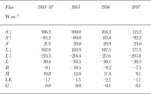
Annual mean values of the surface energy fluxes are given in Table 3. The annual mean fluxes for 1995 are calculated using january and February 1996 to fill in the missing values. The annual mean net radiation flux is negative and is almost equal to the value found by Reference King, Anderson, Smith and MobbsKing and others (1996) of -9.8 W nT² for Halley. The negative net radiation is mainly balanced by a net downward sensible-heat transport. This indicates stable conditions on average. This balance was also found at the South Pole (Reference CarrollCarroll, 1982), but the fluxes were twice as large (H = 19.4 W m⁻², R = -18.7 W m⁻²). The annual mean subsurface energy flux is small and changes sign from year to year. Positive values indicate cooling, and negative values warming, of the snowpack. The calculated annual mean latent-heat flux 0f-1.7 W nT² corresponds to a mass loss through sublimation of 20.0 mm we. a⁻¹. The fluxes are reasonably constant from year to year.

Table 3. Annual mean values and mean values over the 3year period of the surface-energy-flux components

Summary and Concluding Remarks

The AWS on Berkner Island has provided us with a fairly complete 3 year meteorological dataset. The data show that the near-surface conditions on Berkner Island are largely determined by the large-scale flow; the station is located on a dome where it is unaffected by katabatic flows. The annual mean air temperature is about –24°C. In the absence of katabatic forcing, the annual mean wind speed is relatively low (4.5 m s⁻¹) and the wind direction variable (directional constancy 0.38). The annual mean mass balance is positive and about 180 mm we. a⁻¹, which compares well with ice-core studies (Reference WagenbachWagenbach and others, 1994).

Using an energy-balance model, we have computed the surface energy balance and subsurface temperatures. The calculated subsurface temperatures compare reasonably well with the measurements. The sensitivity analysis shows that the subsurface temperatures are especially sensitive to changes in the parameterisation of the incoming longwave energy flux and the magnitude of the extinction coefficient of penetrating shortwave radiation in snow. Nevertheless, considering the limited number of variables measured and the large number of assumptions made, the simulation can be regarded as reasonably good, with mean differences between modelled and measured snow temperatures of –1.0°G at the 0.1 m level and –0.8°C at the 1 m level.

On an annual average the net shortwave radiation flux is the largest positive term (i.e. directed toward the surface) in the energy balance (+21.3 W nT²). The sensible-heat flux is also positive (+10.8 W nT²). The net longwave radiation flux (-30.4 W m⁻²) and the latent-heat flux (-1.7 W m⁻²) cool the surface on average. The annual cycle of the surface energy balance shows that in early summer the sensible-heat flux is negative and heating of the snow occurs. The other months show a steady cooling of the snowpack.

This study shows that using simple meteorological measurements (temperature, wind speed, pressure, incoming shortwave radiation and snow-height changes) and a surface energy-balance model, it is possible to calculate the surface energy fluxes, provided that model input parameters (e.g. surface roughness length and snow conductivity) and parameterisations (e.g. longwave incoming radiation and Monin-Obukhov similarity theory) are known and correct. The accuracy of the calculated fluxes can be improved by improving the parameterisations of the incoming longwave radiation for polar regions and implementing a wavelength-dependent extinction coefficient of shortwave radiation in snow. On the instrumental side, solving the problem of freezing of the wind-speed sensor and increasing the number of observed meteorological parameters (e.g. outgoing shortwave radiation, humidity and longwave radiation) can lead to improvements.