


Abstract
The North Atlantic Ocean is the most intense marine sink for anthropogenic carbon dioxide (CO2) in the world's oceans, showing high variability and substantial changes over recent decades. However, the contribution of biology to the variability and trend of this sink is poorly understood. Here we use in situ plankton measurements, alongside observation-based sea surface CO2 data from 1982 to 2020, to investigate the biological influence on the CO2 sink. Our results demonstrate that long term variability in the CO2 sink in the North Atlantic is associated with changes in phytoplankton abundance and community structure. These data show that within the subpolar regions of the North Atlantic, phytoplankton biomass is increasing, while a decrease is observed in the subtropics, which supports model predictions of climate-driven changes in productivity. These biomass trends are synchronous with increasing temperature, changes in mixing and an increasing uptake of atmospheric CO2 in the subpolar North Atlantic. Our results highlight that phytoplankton play a significant role in the variability as well as the trends of the CO2 uptake from the atmosphere over recent decades.
Export citation and abstract BibTeX RIS

Original content from this work may be used under the terms of the Creative Commons Attribution 4.0 license. Any further distribution of this work must maintain attribution to the author(s) and the title of the work, journal citation and DOI.
1. Introduction
Marine phytoplankton are responsible for approximately half of the primary production on earth [1]. However, little is known about how variable the biological response to interannual changes in ocean circulation is, and how this is influencing the air-sea flux of carbon dioxide (CO2). This is in part due to a lack of in situ measurements [2, 3], which has led to a substantial divergence in future climate model projections [4, 5]. Therefore, quantifying the role of phytoplankton in marine carbon sequestration is critical in understanding the biological impacts of climate change and consequent feedbacks on climate.
Atmospheric CO2 concentrations have increased continuously since the industrial revolution, contributing to rising global temperatures [6]. The North Atlantic Ocean is an important net sink of atmospheric CO2, taking up an estimated 23% of the anthropogenic global carbon inventory, while only covering 15% of the global ocean [7, 8]. CO2 uptake in the North Atlantic is highly variable [9, 10], with air-sea exchange controlled by the partial pressure CO2 (pCO2) gradient between the ocean and the atmosphere, which is influenced by the temperature dependent solubility of CO2 as well as other processes such as physical mixing and biological uptake [10, 11]. While the influence of temperature on the solubility of pCO2 is well understood [11–13], much less process understanding exists regarding the drivers that are not directly related to temperature variations, i.e. the non-thermal drivers, in particular the role of biology. Ocean circulation and mixing control the amount of deep, aged (i.e. carbon and nutrient rich) water reaching the ocean surface [14–16], and therefore modify on large scales, the magnitude of biological production. Seasonal warming and light, as well as nutrient availability, trigger phytoplankton photosynthesis, with consequent increased uptake of CO2 [12] and increase in phytoplankton biomass. Satellite measurements have served as appropriate indicators of the variability in sea-surface chlorophyll-a (chl-a), i.e. a first order proxy for biological production in the top surface layer of the ocean, but are not yet able to differentiate the plankton community composition [17–19]. Here we also use in situ data collected from the Continuous Plankton Recorder (CPR), which utilises a robust marine sampler towed within surface waters at a depth of ∼7 m (sampling the top ∼20 m of seawater due to the wash of the volunteer ships that tow CPRs) and a procedure that has remained consistent since 1958 [20]. This unique dataset allows us to investigate the variability of plankton biomass and community composition in surface waters over multiple decades at large spatial scales, such as that of the North Atlantic Ocean. Combining this with an observation-based estimate of the partial pressure of carbon dioxide (pCO2) at the sea surface [21, 22] from 1982 to 2020 derived from the Surface Ocean CO2 Atlas (SOCAT) [23], we demonstrate the importance of biology on the uptake of carbon in the North Atlantic at seasonal, interannual and decadal time-scales. Further, by investigating changes in temperature and mixing, we provide a more advanced understanding of the processes involved in the drawdown of CO2.
2. Materials and methods
Our main focus here is the basin-wide relationship between phytoplankton and the difference in atmospheric and oceanic CO2 concentrations, i.e. the thermodynamic disequilibrium driving the exchange of CO2 between the atmosphere and the surface ocean of the North Atlantic (See figure S1 for mean values and study area). The air-sea pCO2 difference (pCO − pCO
− pCO =
=  CO2), was calculated using xCO2 atmospheric data obtained from the NOAA marine boundary layer reference network [24]. Phytoplankton groups were defined and quantified using CPR data [20], and diatoms are presented in the main text, however other phytoplankton groupings were considered in the analysis (table S1 within the supplementary extended data lists the phytoplankton taxa that were included in the phytoplankton groupings for diatoms and dinoflagellates. Coccolithophores and silicoflagellates were included as separate groups and were only recorded as presence/absence values until 1993, after which they are routinely speciated and counted within the CPR survey, however their pigment (along with other phytoplankton species' pigment) is detected in the Phytoplankton Colour Index (PCI) signal [20]. Diatoms are also thought to be one of the major phytoplankton groups contributing to the biological uptake and potential export of CO2, due to their relative size (and therefore transfer efficiency to the deep ocean) and dominance of the North Atlantic spring bloom [25, 26].
2.1. Datasets
The carbon observation data were obtained from the SOCAT (www.socat.info) [23]. pCO2 is derived from the fugacity of carbon dioxide (fCO2) [27] and then interpolated using a 2-step neural network technique to provide monthly coverage on a 1 × 1∘ grid [21, 22].
Regional monthly-mean atmospheric xCO2 data were obtained from the NOAA marine boundary layer reference network [24]. This was converted to atmospheric pCO2 following [28]:

where P is the sea-level pressure [29], and  is the water-vapour pressure at 100% humidity [28].
The phytoplankton data were obtained from the CPR Survey (CPR, www.cprsurvey.org). The CPR is a towed marine sampler, that is voluntarily towed behind ships of opportunity at a water depth of ∼7 m, which due to the wash of the ship samples the top ∼20 m surface layer [20]. The mesh size of the silk used within the CPR is 270 µm, and although this means that larger phytoplankton are better represented in the CPR dataset, the CPR does routinely record phytoplankton down to approx. 5–10 µm (such as coccolithophores). In addition, the PCI does reflect some of the smaller taxa as their biomass adds to the colouration of the silk [30]. Satellite derived chl-a was also included in the analysis as an independent measure of phytoplankton biomass within the study area. It is important to note that there are limitations associated with both satellite and CPR measurements for estimating the plankton [18], as with any plankton sampling method [31]. Rare species bias was removed from the CPR dataset by only including taxa that occur above 1% frequency of occurrence [32]. Table S1 within the supplementary extended data lists the taxa that were included in the phytoplankton groups, as well as the use of the PCI. The phytoplankton data were all log transformed using log10 (x + 1) in order to homogenise the variance [33, 34]. Each phytoplankton index was gridded onto a 1 × 1∘ grid by taking the monthly mean for each grid cell, and removing any grid cell where the CPR sample number was  3 to reduce the potential impact of decreased sampling effort [34]. For a detailed methodology on using the CPR data please refer to Richardson et al [20].
The satellite derived estimate of sea surface chl-a was obtained from the OC-CCI dataset version 4.1, which is a merged MERIS, Aqua-MODIS, SeaWiFS and VIIRS global satellite product from 1998–present (esa-oceancolour-cci.org) [35]. The chl-a data were averaged by month on to a 1 × 1∘ grid within the study area for the analysis.
Mean monthly sea surface temperature (SST) data from 1982 to 2020 were obtained from the International Comprehensive Ocean-Atmosphere Data Set (ICOADS, 1∘ enhanced data, www.esrl.noaa.gov/psd/data/gridded/data.coads.1deg.html) [36].
Mixed layer depth (MLD) from 1982 to 2020 was obtained from the global ocean and sea-ice reanalysis products (ORAS5: Ocean Reanalysis System 5) prepared by the European Centre for Medium-Range Weather Forecasts (ECMWF www.ecmwf.int/node/18519) [37] and generated using Copernicus Climate Change Service information (2022). Where MLD is defined as the depth of the ocean where the average sea water density exceeds the near surface density plus 0.01 kg m−3.
2.2. Data collocation
Datasets were spatio-temporally collocated by gridding them at 1 × 1∘ resolution and taking monthly means within each grid cell from 1982 to 2020, with the exceptions of the chl-a dataset which was only available from 1998 onwards. Although CPR data from the North Atlantic are available from 1958 onwards, for comparison with oceanic CO2 data (available from 1982 onwards) the main analyses within this paper focus on the period 1982 to 2020, however phytoplankton trends are presented in figure 6 to aid discussion around multidecadal trends.
2.3. Thermal and non-thermal pCO2 components
Thermal (pCO2T) and non-thermal (pCO2NT) driving components on pCO2 were derived based on the well constrained influence of temperature on pCO2 under fixed dissolved inorganic carbon (DIC) and total alkalinity (TA) conditions, where  ln pCO2/
  T = 0.04 231 ∘C −1 [11–13]:


where the over bar indicates mean parameter. pCO2T calculated following equation (2) represents the pCO2 concentration if the addition or removal of carbon by biological and air-sea exchange processes were absent. pCO2NT (equation (3)) represents the pCO2 concentration due to changes in DIC and TA, which could be influenced by biology, air-sea CO2 exchange, advection, and mixing [13].
2.4. Determination of linear trends and statistical testing
Annual linear trends were calculated for each 1 × 1∘ grid-cell, using standard model I linear regression. The significance of the linear trend was calculated whereby the ratio (tb) of the linear trend (T) and the standard error of the linear trend (SE(Ne)) (equation (5)) were compared to a critical value of t (tcrit, assuming a distribution of student's t) at a 95% significance level and the effective degrees of freedom, which takes into account any autocorrelation within the time-series by using the effective sample size (Ne) [38]:

The most common autocorrelation within time-series is temporal autocorrelation, which implies that throughout time preceding observations are not independent of each other. This has implications for the significance of any trend where temporal autocorrelation exists [39]. To account for temporal autocorrelation when calculating the significance of the linear trends and any correlations within the time-series data, the modified Chelton method was used as it has been shown to be the optimum method for altering significance due to autocorrelation within time-series [39]. Those samples that are not autocorrelated within the time-series are effectively independent and counted within the effective sample size (Ne), which will be less than the sample size (N). By using the effective sample size to calculate the standard error of the linear trend and the critical value of t (rather than N) this reduces the significance of the trends and therefore takes into account autocorrelation within the time-series [40].
2.5. Objective mapping
Objective mapping was used for gap-filling of the CPR values in figures 4(c) and S1(c), for all other visualisations or numerical results no gap-filling technique was used on the CPR data. Objective mapping is similar to kriging and follows the least squares approach, but it assumes that the mean drift (trend) is known and uses a covariance matrix where larger weights are assigned to points that are nearby and co-vary positively with the estimated values [41]. The method can be described by the following equation:

where b is the mapped property, w is the data weights, E is the covariance matrix and r is the residuals (weighted mean) [42].
2.6. Monthly standardised anomalies
Standardised zscore calculation measures the standardisation (distance from the mean using standard deviation) of the data [41]. The output is a standardized zscore where positive values signify values above the long term mean and negative values are below the long term mean, zero values are at the long term mean.
3. Results and discussion
Our analysis reveals that the seasonal diatom abundance maxima occurred concurrently with the seasonal minima in  CO2 (figures 1(a) and (c)). In temperate and subpolar latitudes this occurs during spring. Further south, in the subtropical zone, where temperature dominates the timing of the seasonal carbon maximum [11, 12, 43], diatoms and
  CO2 have their seasonal maximum/minimum shifted towards winter. This confirms that two contrasting mechanisms are affecting the seasonal cycle of CO2 drawdown in the North Atlantic [21, 43]. In higher latitudes, the strongest drawdown of sea surface CO2 is observed during spring (figure 1(a)), initiated by a combination of increasing light levels, rising temperatures (figure 1(b)), and by increased nutrient concentrations brought to the surface by deep wintertime mixing (figure 1(d)). This spring period is associated with a peak in spring-blooming diatoms during May/June (figure 1(c)). At these higher latitudes, there is also a later, weaker CO2 drawdown period in August associated with diatom biomass (figures 1(a) and (c)). In the high latitudes in winter, the seasonal
  CO2 signal (figure 1(a)) is positive, i.e. the surface ocean is supersaturated with CO2 with respect to the atmospheric concentration. This supersaturation is associated with increased turbulence (MLD) (figure 1(d)) that is mixing carbon-rich deeper waters to the surface [13]. As temperatures increase and surface wind speeds decrease in spring, stratification allows the phytoplankton to bloom and take up CO2 via photosynthesis, making the surface ocean CO2 undersaturated with respect to the atmospheric CO2 [13] (negative
  CO2). The seasonal temperature cycle is opposing the sea-surface
  CO2 in the high latitudes (figures 1(a) and (b)), confirming that solubility only plays a secondary role in the
  CO2 seasonality [11, 21, 43]. In contrast, in the lower latitudes, the solubility effect is the dominant process [11], as the seasonal
  CO2 cycle follows the seasonal temperature variability with summer/autumn months being associated with the release of CO2 to the atmosphere from the ocean (figures 1(a) and (b)) [21, 43]. These contrasting mechanisms between the subpolar and subtropical North Atlantic are schematically illustrated in figure 2.

Figure 1. Seasonal variations. Seasonal mean Hovmöller plots of latitude verses time (month) for the North Atlantic (a), ΔpCO2 (µatm) (b), SST (∘C) (c), Diatom abundance (log10(x + 1)) (d), MLD (m). All plots were created using monthly data from 1982 to 2020.
Download figure:
Standard image High-resolution image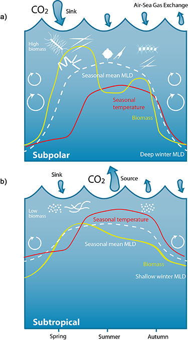
Figure 2. Seasonal schematic. Schematic demonstrating the seasonal changes in temperature (red line), phytoplankton biomass (green line), MLD (white dashed line), mixing (white arrows), and CO2 air-sea gas exchange (blue arrows) in the (a) subpolar North Atlantic, and (b) subtropical North Atlantic.
Download figure:
Standard image High-resolution imageOn interannual time-scales, the comparison between the  CO2 and its drivers (figure 3) illustrates that year-to-year changes in the North Atlantic carbon sink are largely driven by non-thermal effects. Here we derive the temperature independent
  CO2 (non-thermal
  CO2NT, see figure 3(b)) using the temperature sensitivity of CO2 in seawater [11–13] (see Methods). The
  CO2NT represents changes in pCO2 due to non-thermal drivers such as; ocean circulation, mixing, air-sea exchange and biological processes [13]. As the temporal variability of ocean pCO2 is larger than that of atmospheric pCO2 [24, 44, 45], the interannual variability in the
  CO2 is likely to be a product of changes in temperature, ocean physics and biology (figures 3(c), (e) and (g)), and not atmospheric variability. From 2010 onwards, we find a substantial decrease in the seawater
  CO2 and
  CO2NT at ∼50∘ N (figures 3(a) and (b)). This more negative
  CO2 indicates an increased uptake of CO2 by the ocean, which corresponds to an increasing trend in SST, shoaling of the mixed layer and an increase in diatom abundance (figures 3(c), (e) and (g)). We interpret this signal as indicative of shallower mixing depths reducing light limitation, therefore leading to increased photosynthesis, and hence increased uptake of CO2 from the water. The observed increased phytoplankton biomass (figure 6(a)) is dominated by an increase in diatoms (figure 3(c)) and coccolithopheres (figure 6(e)) during this period. The
  CO2 variation and smaller difference between the air-sea pCO2 during the 1990s at 60∘ N (figures 3(a) and (b), ∼60∘ N) aligns with the increased mixing that occurred during this period as the Labrador Sea convection increased [46, 47], bringing carbon-rich waters to the surface and lower diatom abundance due to stronger vertical mixing and hence limited light availability (figures 3(c), (e) and 4(a), (e)). Correlation between diatom abundance and
  CO2NT are negative in the subpolar (⩾45.5∘ N) and positive in the subtropical (
 45.5∘ N) North Atlantic, whilst throughout the majority of the North Atlantic, SST shows a negative correlation with
  CO2 (figure 3(h)), and MLD shows the expected positive correlation with
  CO2NT (figure 3(f)). This confirms the strong link between CO2, phytoplankton biomass and mixing, because if it were just temperature driving the interannual variability you would expect to see a significant positive correlation between
  CO2 and SST across all latitudes.
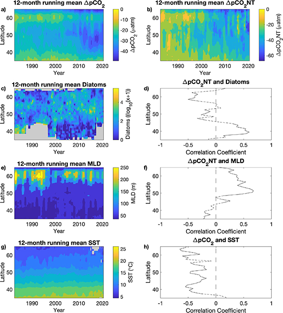
Figure 3. Interannual variations. 12-month running mean Hovmöller plots of latitude verses time (year) for the North Atlantic (a), ΔpCO2 (µatm) (b), ΔpCO2NT (µatm) (c), Diatom abundance (log10(x + 1)) (e), MLD (m) (g), SST (∘C). Areas shaded grey are where there were insufficient data (see Methods). Pearson's linear correlation coefficients at each degree latitude are plotted as a black line for (d), ΔpCO2NT against Diatoms (f), ΔpCO2NT against MLD (h), ΔpCO2 against SST. Correlations that are outside of the 95% significance level ( 0.05) are dashed black lines (see Methods). All plots were created using monthly data from 1982 to 2020.
Download figure:
Standard image High-resolution imageFigure 4 shows maps of the annual linear trends in  CO2, CPR diatom abundance, MLD, SST and satellite derived chl-a estimates for the study area, alongside time-series of the standardised monthly anomalies and linear trends within the the subpolar North Atlantic (⩾45.5∘ N) and the subtropical North Atlantic (
 45.5∘ N) (see Methods). Across most of the North Atlantic the
  CO2 sink is increasing (decreasing trend = more uptake to the ocean), with a significant decrease in
  CO2 seen within the subpolar and subtropical North Atlantic (figures 4(a) and (b)). Although diatom abundance has increased across most of the study area, there is a pattern of decreasing abundance towards the subtropical North Atlantic (figures 4(c) and (d)). This regional biomass trend is also reflected in the PCI (PCI, figure 6), and although the satellite derived chl-a data only started in 1998, an increase in chl-a is also observed across most of the subpolar region (figures 4(i) and (j)). SST has increased across the study area (figures 4(g) and (h)), whereas MLD shows a decrease across most of the subpolar North Atlantic, in particular the western North Atlantic (figure 4(e)). This pronounced shoaling of the mixed layer in the Labrador Sea since the end of the 1990s (figures 4(e) and (f)), coincides with increased diatom abundance which is more pronounced on the western North Atlantic because of a reduction in Labrador Sea convection due to warming [46, 47] (figures 4(c) and (d)). These data support model predictions suggesting that increasing temperature would result in enhanced stratification which would lead to decreased productivity in the subtropics due to increased nutrient limitation and increased productivity in subpolar regions due to decreased light limitation [48–51]. Figures 5 and 6 (phytoplankton groups) depict these regional changes between the subpolar and subtropical North Atlantic, showing how mean seasonality and annual variability change over time (see Methods). Despite no clear correspondence between interannual variability in SST and CO2 (figure 3), we do find a corresponding long term warming trend in the subpolar region that matches a long term increase in the CO2 sink which likely reflects the continued increase in atmospheric pCO2 concentrations [5] (figures 5(a) and (d)). We find a significant decrease in
  CO2 in the higher latitudes of −0.45 ± 0.03 µatm yr−1 implying an increase in the marine carbon sink (figures 4(a), (b) and 5(a)), see supplementary extended data table S2 for trend values and their uncertainties). This sink is associated with increased productivity in the subpolar North Atlantic, increased mixing within the Labrador Sea and decreased mixing within the central subpolar North Atlantic (figures 4(a), (c), (e) and 5, supplementary figure 6 and table S2). In the region defined here as subtropical(
 45.5∘ N), it appears that there has been a shift from a seasonal ocean decrease in CO2 during the summer months when Diatom abundance was high (1980s), to a seasonal increase in CO2 during the summer months (2010–2020) where increased temperatures and low Diatom abundance appear to be dominating the system (figures 5(e)–(h)). Over decadal time periods, regional natural variability is likely to be affecting the processes that influence carbon flux variability with varying influence in different regions of the North Atlantic [22, 52]. In particular, the North Atlantic Oscillation has been shown to influence the circulation between the subtropical and subpolar gyres at the decadal scale [8, 52].

Figure 4. Linear trends. Linear trend maps for; (a), ΔpCO2 (µatm yr−1), (c), Diatom abundance (log10(x + 1) yr−1), (e), MLD (m yr−1), (g), SST (∘C yr−1), (i), chl-a (miiligram m−3 yr−1). Red shades signify an increasing trend while blue shades signify a decreasing trend from 1982–2020, except for chl-a (1998–2020). Areas shaded grey are where there were insufficient data (see Methods).
Download figure:
Standard image High-resolution image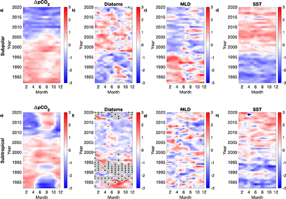
Figure 5. Regional standardised anomalies from 1982–2020. Monthly standardised anomaly plots for the subpolar North Atlantic (⩾45.5∘ N); (a), ΔpCO2 (µatm), (b), diatom abundance (log10(x + 1)), (c) MLD (m), (d), SST (∘C). And for the subtropical North Atlantic ( 45.5∘ N); (e), ΔpCO2 (µatm), (f), diatom abundance (log10(x + 1)), (g) MLD (m), (h), SST (∘C). Red shades signify values above the long term mean and blue shades are values below the long term mean (see Methods). Zero mean values are in white. All plots were created using monthly data from 1982 to 2020. Missing months of data are indicated with a black asterisk.
Download figure:
Standard image High-resolution image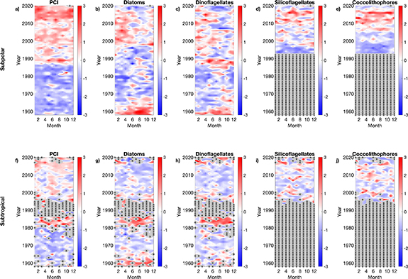
Figure 6. Regional standardised phytoplankton abundance anomalies from 1958 to 2020. Monthly standardised anomaly plots for the subpolar North Atlantic (⩾45.5∘ N); (a) PCI (log10(x + 1)), (b) Diatoms (log10(x + 1)), (c) Dinoflagellates (log10(x + 1)), (d) Silicoflagellates (log10(x + 1)), and (e) Coccolithophores (log10(x + 1)). And for the subtropical North Atlantic ( 45.5∘ N); (f) PCI (log10(x + 1)), (g) Diatoms (log10(x + 1)), (h) Dinoflagellates (log10(x + 1)), (i) Silicoflagellates (log10(x + 1)), and (j) Coccolithophores (log10(x + 1)). Red shades signify values above the long term mean and blue shades are values below the long term mean (see Methods). Zero mean values are in white. All plots were created using monthly data from 1958 to 2020, apart from coccolithophores and silicoflagellates as they were counted within the CPR dataset since 1993. Missing months of data are indicated with a black asterisk.
Download figure:
Standard image High-resolution image
The PCI presents a significant increasing trend across the whole North Atlantic since 1958 (see figure 6). This suggests that smaller phytoplankton taxa ( 5 µm) might be increasing across the whole North Atlantic as they are represented in the PCI but not always recorded in the taxonomic identification process due to the semi-quantitative nature of the CPR sampling (see Methods) and the difficulty of identifying smaller phytoplankton using light microscopy. This observation is supported by both the silicoflagellate and coccolithophore phytoplankton groupings (which generally include smaller taxa than the diatom and dinoflagellate taxa presented (table S1)) showing significant increases in the subpolar region, however their abundance has only been counted since 1993 (figure 6). Changes in dinoflagellate abundance show a similar pattern to that of the diatoms (figure 6), however this could be due to the CPR not quantitatively sampling some of the smaller less-robust dinoflagellate taxa. If modelled predictions of declines in productivity and plankton cell-size are correct [48–51], then it is likely that carbon export and potential sequestration to the deep ocean will be reduced, due to a decreased transfer efficiency [4]. Climatic indices will also likely be influencing multidecadal changes in the phytoplankton [53]. Edwards et al [54] demonstrated that the Atlantic Multidecadal Oscillation (AMO) coupled with the Northern Hemisphere Temperature anomaly is a strong driver of diatom abundance in the northeast Atlantic. These results support our findings, as we see a shift during the 1990s in all of our phytoplankton groupings (see figure 6) which coincides with when the AMO shifts from a negative phase to a positive phase alongside increasing temperatures. This natural climate variability, coupled with warming due to climate change is therefore likely adding to the strength of the trends reported here and demonstrates the regional complexity needed for global models.
4. Conclusion
Our results indicate that marine primary production does not simply affect the (sub-) annual ocean uptake of CO2 from the atmosphere, but it also significantly correlates with the long term variability of this uptake. Our observation-based study agrees with past productivity modelling studies, which have suggested opposing trends in productivity between the subpolar and subtropical North Atlantic [48–51]. However, if the current temperature trajectory and changes in mixing conditions continues, then global declines of productivity could occur, as the balance between relief of light limitation and strengthening nutrient limitation caused by stronger and longer stratification, is altered [51, 55]. The varying influence (from seasonal to multidecadal) of biology on the variability of carbon uptake should be included in models aiming to predict future carbon uptake scenarios. The current ability to represent biological processes in global marine models is limited [56], yet essential for capturing the variability of our climate at multidecadal scales. Although our correlation analysis does not permit us to further untangle the non-thermal drivers and quantify the relative contributions of biology and physics separately, it is encouraging that these data, derived from independent sources and in situ observations, complement each other so clearly, and are consistent with our understanding and model predictions of the system. Our results highlight that phytoplankton play a fundamental role in ocean carbon uptake and its long term variability, therefore regulating the earth's climate. The role of phytoplankton role in this process is dictated by the community composition (predominantly diatoms in the North Atlantic), the latitude (subpolar systems drawing down more carbon) and by large-scale hydro-climatic processes operating over multidecadal scales. Only by the sustained and coordinated monitoring of these oceanic biogeochemical parameters and plankton communities can we improve our understanding of future climate change impacts and the role of the ocean in planetary feedback mechanisms, which are currently poorly constrained in areas with complex bio-physical interactions of carbon uptake.
Acknowledgments
Funding that supports the running of the Volunteer Observing Shipping network used in this project includes EU 264879 (CARBOCHANGE), EU Grant 212196 (COCOS), and UK NERC Grant NE/H017046/1 (UKOARP), DEFRA UK ME-5308, NSF USA OCE-1657887, DFO CA F5955-150026/001/HAL, Climate Linked Atlantic Sector Science (CLASS) UK NERC Grant NE/R015953/1, Horizon 2020: 862428 Atlantic Mission, IMR Norway, and DTU Aqua Denmark. Funding for this project was provided by NERC Grant reference NE/J500069/1. P L is supported by the Max Planck Society for the Advancement of Science. M J was supported by NERC Grant NE/K00168X/1 (Data Synthesis and Management of Marine and Coastal Carbon). We thank the many people and funding agencies responsible for the quality control and collection of data for their invaluable work and contributions.
Data availability statement
The data that support the findings of this study are available upon reasonable request from the authors. The datasets that support the findings of this study are available through the following listed websites; the carbon observation data were obtained from the SOCAT (www.socat.info), the biological data were obtained from the CPR Survey (www.cprsurvey.org), SST data were obtained from the ICOADS (1∘ enhanced data, www.esrl.noaa.gov/psd/data/gridded/data.coads.1deg.html). The satellite derived estimate of sea surface chl-a was obtained from the OC-CCI dataset version 4.1 (esa-oceancolour-cci.org) [35]. MLD was obtained from the global ocean and sea-ice reanalysis products (ORAS5: Ocean Reanalysis System 5) prepared by the European Centre for Medium-Range Weather Forecasts (ECMWF www.ecmwf.int/node/18519) [37].
Author contributions
C R, U S, M E conceived the project, P L developed the neural network analysis, C O collated the data, did the computations and data analysis and prepared the first draft of the manuscript. A J W provided expertise on ocean circulation and biogeochemical processes, M J, S S and P L provided expertise on computations. M E developed the illustrative schematic. All authors contributed to the discussion of the results and reviewed the manuscript.
Conflict of interest
The authors declare that they have no conflicts of interests.
Supplementary data (0.5 MB PDF)