

Abstract
Widespread mismatches between proxy-based and modelling studies of the Last Glacial Maximum (LGM) has limited better understanding about interglacial-glacial climate change. In this study, we incorporate non-breaking surface waves (NBW) induced mixing into an ocean model to assess the potential role of waves in changing a simulation of LGM upper oceans. Our results show a substantial 40 m subsurface warming introduced by surface waves in LGM summer, with larger magnitudes relative to the present-day ocean. At the ocean surface, according to the comparison between the proxy data and our simulations, the incorporation of the surface wave process into models can potentially decrease the model-data discrepancy for the LGM ocean. Therefore, our findings suggest that the inclusion of NBW is helpful in simulating glacial oceans.
Export citation and abstract BibTeX RIS

Original content from this work may be used under the terms of the Creative Commons Attribution 4.0 license. Any further distribution of this work must maintain attribution to the author(s) and the title of the work, journal citation and DOI.
1. Introduction
Surface waves are a ubiquitous process in the upper ocean. The concomitant orbital motion of water particles related to non-breaking surface waves (NBW) generates turbulence and hence vertical mixing even without wave breaking (Qiao et al 2004, 2016, Babanin 2006). The introduction of NBW-induced mixing into simulations of the present-day (PD) ocean has proven to be an effective way in decreasing long-standing ocean modelling biases, including reducing the warm bias in the mid-latitude surface and the cold bias in the subsurface, especially for the summer (Qiao et al 2004). Moreover, the amelioration via NBW processes can be further amplified by air-sea coupling feedbacks in the climate system, as indicated by the experiments using Earth system models (Song et al 2012a), and thus also helpful to decrease climate-modelling biases.
Despite the fact that the incorporation of NBW-induced mixing into ocean models can improve PD simulations, its role in changing simulations of other climate backgrounds, such as the Last Glacial Maximum (LGM), is still unknown. The LGM (∼21 ka BP) is an episode when North America and the Eurasia were covered by large ice sheets (Clark et al 2009) and atmospheric and oceanic circulations were totally different from the modern climate. Reconstructing the LGM ocean climatology is therefore important for understanding the climate history under forcings (e.g. low CO2 levels and large ice sheets) that were different from today. The strongly distorted external forcings have also made LGM a perfect testbed for evaluating numerical climate models, due mainly to abundant geological data and the precise orbital forcing for the LGM (Berger 1978, Braconnot et al 2012).
The upper ocean interacts directly with the atmosphere and plays important roles in shaping the LGM climate. In order to infer information about upper ocean temperatures in the past, we employ proxy-based paleothermometers. We can, for example, use oxygen isotopic ratios in planktonic foraminifera to reconstruct LGM sea surface temperature (SST). The alkenone unsaturation ratio also serves as a good indicator of the annual mean SST (Tierney 2012). Recently, synthetic global data sets, such as the MARGO data set (the Multiproxy Approach for the Reconstruction of the Glacial Ocean Surface project; Waelbroeck et al 2009), have provided a combination of multi-proxy approaches and different transfer function techniques to create a robust reconstruction of the LGM surface ocean. Complementary to the proxy-based temperature determination at scattered locations are model-based simulations. The employment of numerical models permits us the possibility of unifying sparse reconstructed temperatures and creating a full map of the global LGM ocean. Numerical models avoid interpolation of geographically sparse proxies and keep the ocean more physically dynamical constrained (Paul and Schäfer-Neth 2005). Within the Coupled Model Intercomparison Project (CMIP), LGM simulations have become an important benchmark for testing climate models (Taylor et al 2012). In recent years, combining proxies and models has become an effective way of reconstructing the LGM SST. By doing so, we are able, for example, to retrieve large-scale LGM SST patterns in detail. Although a plausible first-order model-proxy consistency, such as the overall land-sea contrast and polar amplification, has been achieved, there are still noticeable mismatches between proxy reconstructions and model simulations. Models tend to simulate weaker LGM cooling than the expected (Braconnot et al 2012). The inter- and intra-basin variations of the LGM cooling (Otto-Bliesner et al 2009), in other words, the spatial heterogeneity of the proxy, are also underestimated by models (Harrison et al 2014). From the Paleoclimate Modelling Intercomparison Project Phase 2 (PMIP2) to PMIP3, the model-proxy bias was not obviously improved even with models of increased complexity and resolution (Harrison et al 2014).
According to numerical results (Shin et al 2003) and terrestrial and marine paleo-evidence (Kohfeld et al 2013), the wind could have been much stronger in the LGM than it is for today. So we expect there could be stronger NBW-mixing and thus greater NBW-induced impact on the LGM ocean. Here we use numerical simulations to demonstrate the potential role of the NBW in changing the LGM upper-ocean temperature simulations.
2. Model and data
In this study, we examine the pure NBW-induced mixing effect on the LGM upper oceans. Therefore, an ocean standalone model, the Finite Element Sea ice-Ocean Model (FESOM, Danilov et al 2004, Wang et al 2008, Timmermann et al 2009) is employed to exclude ocean-atmosphere feedback processes. The model uses multiple resolutions on unstructured meshes. NBW-induced mixing coefficients are generated by the MASNUM wave model (the MArine Science and NUmerical Modeling surface wave model; Qiao et al 2004) and then are added to FESOM. The introduction of NBW to improve PD ocean simulations of FESOM was demonstrated by Wang et al (2019).
We use the same mesh as in Wang et al (2019) for the PD simulation, which has a nominal horizontal resolutions of about 1° for most of the global ocean, 1/3° in the equatorial band as well as 1/3°–1/2° along the coasts (figure S1 (available online at stacks.iop.org/ERL/16/034008/mmedia), left). This mesh has been used in the Coordinated Ocean-ice Reference Experiments phase 2 (CORE II) model intercomparison project (Wang et al 2016). For the LGM mesh, only ocean points in coastal regions affected by a ∼120 m LGM sea level drop are removed (based on the land-sea mask of the ICE_6 G-C reconstruction by Peltier et al (2015), while grid points in the open oceans are unchanged from the PD mesh (figure S1, right). We hypothesize that the NBW-induced mixing is completely suppressed where sea-ice concentrations are greater than 15%. More complex wave-sea ice interaction processes, such as the scattering and dissipation of waves due to sea ice, are beyond the scope of this paper.
For the PD simulations, we use the interannually varying CORE II forcing data set from 1948 to 2009 (Large and Yeager 2009) as the upper boundary condition of the wave as well as the ocean circulation model. We initialize the PD experiments using the temperature and salinity climatology from the Polar Science Center Hydrographic Climatology v.3 (PHC3.0; Steele et al 2001). For the LGM, we run the Max Planck Institute for Meteorology Earth System Model (MPI-ESM, Giorgetta et al 2013) with the PMIP3 experimental setup for the LGM (see http://pmip3.lsce.ipsl.fr/ for detailed information). The model reached a quasi-equilibrium state after more than 4000 model years (Gong et al 2019). The MPI-ESM outputs, including wind speed, specific humidity and temperature at 10 m, sea level pressure, downwelling shortwave and longwave radiation at sea surface, precipitation, and sea level pressure, are then employed to force the wave model and the ocean model. In order to acquire a reasonable seasonal cycle for the LGM forcing, we add the variability of the CORE II data set (1948–2009) to the LGM monthly climatology so that a 62 year LGM forcing is created. The climatologic temperature and salinity from the MPI-ESM ocean are used as the initial conditions of the LGM FESOM simulation. Furthermore, sea surface salinity restoring is used to weaken unbounded local salinity trends due, for example, to inaccurate precipitation and river runoff into the ocean, and to avoid the effect of mixed boundary conditions in the ocean model (e.g. Lohmann et al 1996). We restore the sea surface salinity (SSS) to PHC3.0 data for the PD simulation, and to the monthly climatological salinity from MPI-ESM for the LGM simulation with the strength of SSS restoring being 30 m over 180 d (defined by a piston velocity). Twin experiments, with and without surface waves, are carried out (table 1). In each experiment, four 62 year cycles of integration are performed sequentially, thus allowing for fully developed upper ocean circulation in the ocean model. Then we compare the results of the last-cycle simulation to the LGM (MARGO) and the PD data (World Ocean Atlas 2013, WOA13, Locarnini et al 2013).
Table 1. List of ocean simulations and their setups. 'MPI-ESM + CORE II' means the monthly atmospheric climatology of MPI-ESM and the variability of CORE II are combined to create the LGM forcing.
| Experiment ID | Forcing | Initialization | NBW-induced mixing |
|---|---|---|---|
| pd | CORE II | PHC3.0 | No |
| pd_wave | CORE II | PHC3.0 | Yes |
| lgm | MPIESM + CORE II | MPIESM ocean climatology | No |
| lgm_wave | MPIESM + CORE II | MPIESM ocean climatology | Yes |
3. Results
As the strong-wind belt in the winter migrates across hemispheres seasonally, the NBW-induced mixing coefficient traces the wind patterns on the ocean surface (figure 1): stronger winds during the winter tend to create larger vertical mixing coefficients. In the Southern Ocean, the NBW generated by the perennial westerlies introduces considerable mixing during the whole year. The NBW mixing coefficients have small difference (<0.05 m2 s−1) for the LGM and PD in the boreal summer, while in the boreal winter the NBW creates larger mixing coefficients (0.3 m2 s−1) during the LGM, especially in the North Atlantic Ocean.
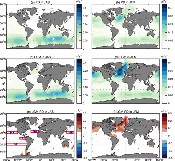
Figure 1. The non-breaking waves induced mixing coefficients (a)–(d) and the difference between the LGM and the PD (e), (f). (a), (c), (e) JAS (July, August and September); (b), (d), (f) JFM (January, February and March). The red boxes in panel e are ocean regions where field-mean results are calculated in figure 3. NP, the North Pacific; SP, the South Pacific; ETP, the eastern Tropical Pacific; NA, the North Atlantic.
Download figure:
Standard image High-resolution imageIn summer, the NBW mixing brings the excessive heat at surface to subsurface (40 m depth), hence cooling the surface and warming the subsurface. The mid-latitude oceans warm by about 1.5 °C–3.0 °C (figures 2(a)–(d)). Subsurface temperatures in the eastern Tropical Pacific and the eastern Tropical Atlantic are also significantly heated by the NBW. The LGM and PD subsurface warming shares similar patterns, but with different amplitudes. In the LGM, NBW creates more summertime subsurface warming in the midlatitudes and more year-round warming in the eastern Tropical Atlantic, but less warming in the North Atlantic and the Southern Ocean (figures 2(e) and (f)).

Figure 2. The non-breaking wave-induced subsurface (40 m depth) temperature change (a)–(d) and the difference between the LGM and the PD (e), (f).
Download figure:
Standard image High-resolution imageNBW plays a role in heating the subsurface layer and thus reduces simulated biases mainly in the mid-latitude oceans and in the eastern Tropical Pacific (figure 2, see also Wang et al 2019). We select four regions to quantify the surface waves-induced subsurface warming. We use the WOA13 temperature as the 'observation' of the PD ocean. In the PD mid-latitude oceans, a perennial cold bias exists in the subsurface layer which peaks in local summer (figures 3(a), (c) and (e)). The NBW-induced subsurface warming, which also reaches maximum in summer, leads to an improvement of the subsurface simulation for the entire year. In the mid-latitude oceans, the simulated subsurface temperatures fit well to the observed ones, when the NBW-driven mixing process is considered in the ocean model (figures 3(a), (c) and (e)). In the eastern Tropical Pacific, the simulated subsurface temperatures, whether the NBW is coupled with the ocean model or not, exhibit much larger seasonal variability than the WOA13 (figure 3(g)). NBW ameliorates the simulation with 1.0 °C–2.0 °C warming almost all year round. In May and June, the NBW-induced warming deteriorates the model, overestimating the temperature of the subsurface layer. The simulated subsurface temperatures in mid-latitude LGM oceans show an overall decrease relative to the PD (red lines in figure 3), especially in the Pacific. In the LGM, NBW exerts a similar seasonal warming pattern on the subsurface, but with a larger amplitude. For example, in the North Pacific Ocean, the summer warming reached 2.0 °C in the LGM while it is only 1.0 °C in the PD (figures 3(a) and (b)). In fact, the warming effects shown in figure 3 (blue lines) are field-mean results over large regions. For specific small ocean areas, the NBW-induced temperature change in LGM can reach as much as 3.0 °C (figure 2).
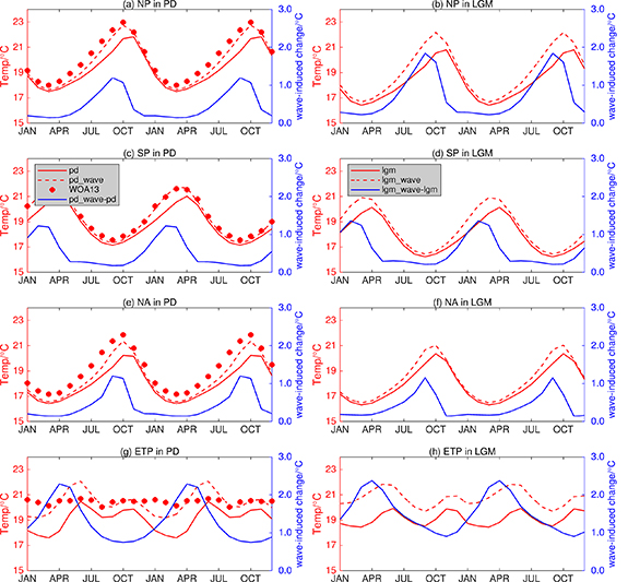
Figure 3. The LGM and PD subsurface temperatures in (a), (b) the North Pacific, (c), (d) the South Pacific, (e), (f) the North Atlantic and (g), (h) the Eastern Tropical Pacific. Two annual cycles are plotted to clearly show the seasonality. Field-mean temperatures are calculated in corresponding regions shown in figure 1(e). The solid red line is the simulated temperature without wave and the dashed red line is the simulated temperature with wave incorporated into the ocean model. The blue line is the wave-induced temperature change, i.e. the difference between the two red lines. The red dots are field-mean climatologic temperatures (1955–2004) of WOA13 in the respective month.
Download figure:
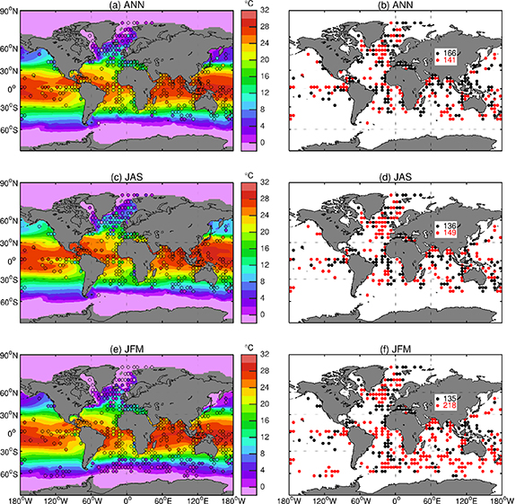
Standard image High-resolution imageHere we make a comparison between the model-based and proxy-based LGM SSTs. We interpolate the modelling results onto the 5° × 5° MARGO grid and then compare the simulated 10 m depth temperatures to temperatures reconstructed from proxies (figure 4; see also the LGM-PD anomaly in figure S2). Overall the first-order SST patterns recorded by the proxy, such as the warm LGM-PD anomaly in the eastern Tropical Pacific and the large east-west SST gradients in the North Atlantic (Waelbroeck et al 2009), are well reproduced by our model (figures 4(a), (c) and (e)). In addition, we successfully reproduce the warmer SSTs in the Nordic Sea indicated by the proxy (figure S2). On the other hand, notable model-data discrepancy exists in the central North Atlantic where our model simulates warm SST anomalies while the proxy indicates colder SSTs during the LGM, especially during the boreal winter (figures 4(e) and S2(e)).
Figure 4. The simulated LGM SSTs and the effect of non-breaking waves in changing the SST simulation. (a), (c), (e) SSTs reconstructed by MARGO (the dots) and by the model run lgm_wave (the shading); (b), (d), (f) the impact of NBW on the mode-proxy biases. Red points means the incorporation of non-breaking waves decreases the model-proxy discrepancy while black ones increase it. (Inset) The total number of red and black points.
Download figure:
Standard image High-resolution image
4. Discussion and conclusion
The stronger surface waves-related mixing in the LGM (figure 1) is a direct reflection of the stronger winds at that time compared to the PD. Numerical simulations have shown the vital role of the orography of the LGM Laurentide Ice Sheet in steering the westerly winds (Oster et al 2015) and intensifying the surface wind over the North Atlantic Ocean (Gong et al 2015). In the LGM, when the core of the westerlies shifted southward (Arpe et al 2011), the zonal-mean wind stress over the North Atlantic was distinctly enlarged (Shin et al 2003).
Although the NBW-induced mixing is much stronger in winter than in summer, the wave-generated ocean warming at subsurface happens in summer (figure 2). This is because in the model, it is not the mixing coefficient alone, but its multiplication with the vertical temperature gradient that changes the upper-ocean temperature (Wang et al 2019). In summer, the heated surface water sits on relatively cold water, resulting in strong and stable stratification and hence great vertical temperature gradients in the upper ocean. Therefore, the NBW-induced temperature change at the subsurface mainly occurs in summer. The mixing in the LGM boreal summer is only a little stronger than that in the PD (figure 1(e)), but this difference of mixing can introduce a considerable temperature change (figure 2(e)).
The NBW-induced mixing has improved half of the modelled SSTs, but makes the other half worse (figures 4(b), (d) and (f)). Some of the deteriorated SSTs due to wave reside in the Mediterranean Sea where the roles of NBW in affecting the ocean simulation is not yet understood. In addition, the NBW-induced improvement and exacerbation in figure 4 depends heavily on the simulated LGM background state. We cannot expect to decrease the model-data difference simply by cooling the simulated summer and warming the winter (see the impact of the NBW on the ocean surface in figure S3), although if we combine the summer and winter on the respective hemisphere together (figure S4), the NBW does show more a positive role in the summer.
Another feature of NBW in the LGM is that there is less prominent subsurface warming around Antarctica. This is counterintuitive in that we expect a more intense subsurface warming due to strong wind-driven wave processes. Both model simulations (Sime et al 2013) and proxy evidence (Kohfeld et al 2013) indicate that there was a stronger westerly belt across the Antarctic Circumpolar Current region. A potential explanation for this is the presence of relatively thick sea ice cover during the LGM. In our model setups, we assume a cutoff of NBW where sea ice concentration is greater than 15%. The thick and compacted sea ice in the Southern Ocean should have weakened the wave processes therein during the LGM.
In the North Atlantic Ocean, the NBW-induced warming signal in LGM at subsurface is weaker by more than −1.6 °C in the boreal summer than the PD warming (figure 2(e)). This weaker LGM warming should not have resulted from sea ice cover, given that in summer this region is almost ice free in both the LGM and PD (Stärz et al 2012). One possible explanation is that our model simulates excessively warm LGM SSTs in this region (figures 4 and S2), resulting in an overly stable stratification that hinders the wave-induced heat transfer from the surface to the subsurface. The incomplete representation of mesoscale eddies in the model, due to the difficulty in parameterizing eddy processes in the upper ocean (Canuto and Dubovikov 2011) and the relatively coarse resolution we are using, could also be a cause of the temperature anomaly in the northwest North Atlantic Ocean.
For the ocean standalone model without air-sea feedbacks, SST is determined largely by the atmospheric forcing. Therefore, the SST changes (figures 4 and S3) are of rather small amplitudes (mostly less than 0.5 °C), and only shows a qualitative rather than a significant improvement compared to the uncertainty of proxy data. This minor change in SSTs, however, will be amplified through air-sea feedbacks in coupled climate models (Song et al 2012b). Therefore, a fully coupled climate model with the NBW process could produce larger changes in an LGM simulation.
In this paper we try to differentiate the surface temperature change from that of the subsurface (40 m depth). Nevertheless, most of the proxy data cannot discriminate between the surface temperature and the temperature at 40 m. Sometimes the term 'subsurface' may stand for a depth range from tens of meters to 200 m (e.g. Tierney 2012, Husum and Hald 2013). In addition, relative to the various proxies for SST reconstructions, only a few proxies exist for subsurface temperature reconstruction. While most of the planktonic foraminifera inhabiting in the low and mid latitudes produce proxies that reflect the SST, some species in the high latitudes might be a proxy of subsurface temperature (Husum and Hald 2013). The temperature proxy TEX86, which is based on the relative cyclization of marine archaeal glycerol dialkyl glycerol tetraether (GDGT) lipids, may represent the subsurface conditions. However, TEX86 may also represent the mean temperature across a time and spatial range, rather than the temperature of a specific layer in a specific month or season, making the comparison with model results difficult. In this paper we chose the 10 m depth temperature as a comparison to MARGO and this presents the same problem. We did not consider the temporal shifts in growing season or vertical shifts in depth habitat of proxies, while considering these shifts could remove some of the model-proxy discrepancies (Lohmann et al 2013).
The lack of temperature reconstructions for the subsurface imposes restrictions on evaluating the impact of the NBW-induced warming on the LGM ocean subsurface. The NBW mixing, at least according to its impact on modern-day oceans, is an important process in the upper ocean. Its incorporation into ocean models is able to reduce the simulated cold bias at subsurface by more than 3.0 °C (figure 2). Compared to the summertime improvement of SSTs, NBW brings heat from surface to subsurface in summer and the extra heat is trapped at subsurface until winter, thus creating an almost all-year-round subsurface warming. More importantly, the mixing coefficient is a derivation directly from the wave-related physical processes (Qiao et al 2010, 2016) which introduces no additional tuning process. That is to say, the improvement resulting from the NBW mixing is universal (Lin et al 2006, Sutherland et al 2013, Fan and Griffies 2014, Ghantous and Babanin 2014, Wang et al 2019), independent of the ocean model type (structured and unstructured) and the climate background (paleo, modern and future). Given the fact that the increase of the complexity and resolution of models barely changes the model-data mismatch between PMIP2 and PMIP3 (Harrison et al 2014), we speculate some important processes, including the non-breaking surface waves in the climate system, might be overlooked. Therefore, we recommend that ocean models take this mixing process into consideration for paleo ocean and climate simulations.
Acknowledgments
The authors declare that they have no conflict of interest.
We thank Dr Patrick Scholz for helping us to plot the resolution map of figure S1. Part of the simulation results which are used in the paper are available online (http://data.fio.org.cn/qiaofl/WSZ-ERL-2021/fesom_wave.tar.gz). The entire simulation results are available from the corresponding author upon request. The source code of FESOM can be downloaded online after registration (https://swrepo1.awi.de/projects/fesom/). The MPI-ESM climate model codes are available online after registration (www.mpimet.mpg.de/en/science/models/license). Thanks go to MARGO (https://epic.awi.de/id/eprint/30068) and World Ocean Atlas 2013 (https://climatedataguide.ucar.edu/climate-data/world-ocean-atlas-2013-woa13) contributor for making the data available. S Wang and F Qiao are supported by the National Natural Science Foundation of China under Grant 41821004. X Gong thank Chinese Minister of Science and Technology Fund (2019YFE0125000), G Lohmann thanks the German BMBF grants PalMod (No. 01LP1504A) and NOPAWAC (No. 03F0785A). G Lohmann, X Gong, E Gowan, and J Streffing receive funding though Helmholtz and BMBF. We thank the two anonymous reviewers for their helpful suggestions to our paper.
Data availability statement
The data that support the findings of this study are openly available at the following URL/DOI: http://data.fio.org.cn/qiaofl/WSZ-ERL-2021/fesom_wave.tar.gz.