


Introduction
Ice shelves buttress and stabilize the continental ice sheet. When ice shelves collapse or thin, the buttressing effect can ease or is even completely lost and ice streams draining the grounded ice sheet may accelerate significantly (e.g. Scambos and others, Reference Scambos, Bohlander, Shuman and Skvarca2004). A reliable understanding of ice shelf dynamics is therefore important for modeling future ice-sheet evolution and its contribution to global sea level change. One of the major factors influencing the ice shelf dynamics is the ocean tide (Padman and others, Reference Padman, Siegfried and Fricker2018). Tides are a direct external force continuously acting on ice shelves and have a large range of effects, some of which we are describing in the following paragraphs. Tides force the ice to bend as it rises and falls together with the ocean it floats in (e.g. Vaughan, Reference Vaughan1995; Fricker and others, Reference Fricker2009), generating fractures via which water and heat are exchanged between the ocean and the ice shelf interior (Joughin and others, Reference Joughin, Alley and Holland2012). Tidal forcing also causes a cyclic migration of grounding lines (Brunt and others, Reference Brunt, Fricker and Padman2011). Models have shown that tides also change the spatial distribution of melting at the ice–ocean interface at large cold-water ice shelves and that estimates of the total mass loss of some ice shelves can double when tides are included in calculations (Makinson and others, Reference Makinson, Holland, Jenkins, Nicholls and Holland2011; Mueller and others, Reference Mueller2012; Gwyther and others, Reference Gwyther2016; Hausmann and others, Reference Hausmann2020). Tides can not only enhance ice shelf melting, but can also enhance ocean circulation within the cavity and meltwater export as reported for the Filchner–Ronne Ice Shelf (Hausmann and others, Reference Hausmann2020). For the Filchner–Ronne Ice Shelf, modeling shows that the tide increases the flow velocity of the ice shelf, on average, by 21% (Rosier and Gudmundsson, Reference Rosier and Gudmundsson2020). Tidal forcing of ice shelves can therefore significantly influence ice-sheet mass balance, because grounded ice stream velocity is affected by ice shelf velocity and buttressing effects. Tides impact the flow of sea water beneath the ice sheet at grounding lines, which are the most vulnerable areas for the mass loss of grounded ice (Walker and others, Reference Walker, Dupont, Parizek and Alley2008; Begeman and others, Reference Begeman2020). Increased grounding line melting significantly increases grounding line retreat. Tidal flexure and the hydrodynamic pressure gradient across the grounding zone can suck salt water into the subglacial hydrology network where it alters basal lubrication, sediment flow and till strength, which influences ice stream velocities landward of the grounding line (Walker and others, Reference Walker2013; Warburton and others, Reference Warburton, Hewitt and Neufeld2020).
Tides are also linked with so-called icequakes (e.g. Podolskiy and Walter, Reference Podolskiy and Walter2016; Aster and Winberry, Reference Aster and Winberry2017; Padman and others, Reference Padman, Siegfried and Fricker2018, and references therein). Icequakes are seismic events whose sources lie within the ice or at the ice–bed boundary. Source mechanisms for icequakes are diverse, such that icequakes occur in a broad frequency range: from 10−3 Hz long-period teleseismically detectable glacial earthquakes to 100 Hz signals caused by icefalls or the opening of cracks and crevasses that are only recorded over distances of a few kilometers (Anandakrishnan and Alley, Reference Anandakrishnan and Alley1997; Sinadinovski and others, Reference Sinadinovski, Muirhead, Leonard, Spiliopoulos and Jepsen1999; Wiens and others, Reference Wiens, Anandakrishnan, Winberry and King2008; Lough and others, Reference Lough, Barcheck, Wiens, Nyblade and Anandakrishnan2015; Podolskiy and Walter, Reference Podolskiy and Walter2016). Some icequake source mechanisms are related to tidal forcing. Tide-induced vertical displacement of the floating ice shelf causes bending near the grounding zone, inducing stress that may lead to brittle failure at the outer bend and therefore flexure-related icequakes. Tides influence cracks and crevasses to open at the base and surface of the ice, generating seismic signals (Hammer and others, Reference Hammer, Ohrnberger and Schlindwein2015; Hulbe and others, Reference Hulbe2016). Other icequakes are related to ice sliding across the bed rock at pinning points (Pirli and others, Reference Pirli, Hainzl, Schweitzer, Köhler and Dahm2018), and the potential for these events changes as vertical tidal movement increases and decreases the area of ice–rock contact.
Tidal forcing not only affects floating ice shelves, but also grounded ice inland. Some ice streams do not move evenly, but instead display tidally modulated stick–slip behavior (Anandakrishnan and Alley, Reference Anandakrishnan and Alley1997; Bindschadler and others, Reference Bindschadler, King, Alley, Anandakrishnan and Padman2003; Wiens and others, Reference Wiens, Anandakrishnan, Winberry and King2008; Winberry and others, Reference Winberry, Anandakrishnan, Alley, Bindschadler and King2009). Depending on the ice bed conditions, the effects of tidal forcing may be transmitted along grounded ice streams to be expressed seismically at distances of as much as 300 km inland of the grounding line (Harrison and others, Reference Harrison, Echelmeyer and Engelhardt1993). Tide-related variations are not only seen in seismological data but also in ice stream velocity and displacement data recorded with GNSS receivers deployed on both grounded ice and floating ice shelves (e.g. Anandakrishnan and others, Reference Anandakrishnan, Voigt, Alley and King2003; Minowa and others, Reference Minowa, Podolskiy and Sugiyama2019). The reasons for the velocity modulations are still not understood in detail, with several processes under discussion. One effect modulating ice flow relates to the changes tides induce in the locations of pinning points and grounding lines, which directly influence buttressing forces and, in turn, induce ice flow variations (Robel and others, Reference Robel, Tsai, Minchew and Simons2017; Rosier and Gudmundsson, Reference Rosier and Gudmundsson2020). Other effects are attributed to the tidally induced changes in ice/water friction at the ice shelves (Doake and others, Reference Doake2002), changes in basal shear traction beneath ice streams (Minchew and others, Reference Minchew, Simons, Riel and Milillo2017) or tilting of the ocean surface (King and others, Reference King2011; Makinson and others, Reference Makinson, King, Nicholls and Hilmar Gudmundsson2012).
Most glaciological studies that consider tidal forcing focus on the main diurnal (~1 cycles per day (cpd): K1, O1, P1, Q1) and semi-diurnal (~2 cpd: M2, S2, N2, K2) tidal harmonics that exhibit the largest amplitudes (e.g. Winberry and others, Reference Winberry, Anandakrishnan, Alley, Bindschadler and King2009; Hammer and others, Reference Hammer, Ohrnberger and Schlindwein2015; Pirli and others, Reference Pirli, Hainzl, Schweitzer, Köhler and Dahm2018). However, additional higher tidal harmonics (also called compound tides or overharmonics) are generated by non-linear interactions of the main tidal harmonics: e.g. interaction of M2 and S2 generates the MS4 harmonic, interaction of M2 with itself can produce M4, interaction of M2 and K1 generates the MK3 harmonic and so on. These overharmonics can occur, e.g. in shallow waters, in areas of complex bathymetry or as a result of ice–ocean interactions.
In this paper we refer to high-frequency tides (>2cpd) or overharmonics also as HF tides. Oceanographic models can include HF tides (e.g. Rosier and others, Reference Rosier, Green, Scourse and Winkelmann2014) but often they are not resolved by the models (e.g. Kagan and others, Reference Kagan, Romanenkov and Sofina2008; Howard and others, Reference Howard, Erofeeva and Padman2019).
The analysis of modern seismic and GNSS data can reveal how Antarctica's ice shelves respond non-linearly to the tidal forcing and, in particular, on the role of HF tides. Here, we investigate tidal forcing of icequake activity and ice velocity by analyzing data recorded on the Ekström Ice Shelf in Dronning Maud Land, East Antarctica (Fig. 1). In our work we have paid particular attention to signals with ~3 cpd and ~4 cpd periodicities and demonstrate that these frequencies are very pronounced in icequake activity and the movement of the Ekström Ice Shelf.
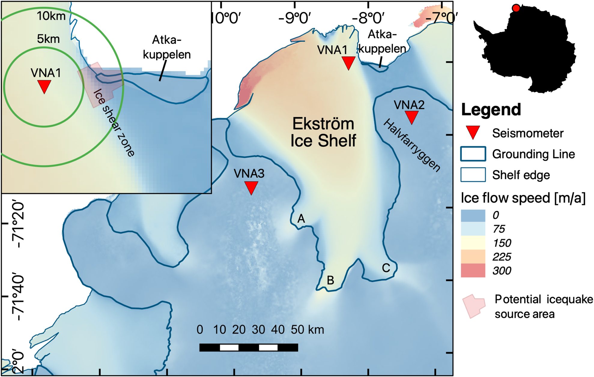
Fig. 1. Map of the working area at the Ekström Ice Shelf with ice flow velocities and seismometer positions. VNA1 is close to Neumayer Station III (Rignot and others, Reference Rignot, Rignot, Mouginot and Scheuchl’2011; Mouginot and others, Reference Mouginot, Scheuchl and Rignot2012). The green circles around VNA1 mark distances of 5–10 km from the seismometer. The ice shelf is fed by three unnamed ice streams labeled A–C.
Methods and datasets
We analyzed a year-long seismological and 10 month long GNSS dataset for 2020, both recorded at Neumayer Station III (Fig. 1). After different preparatory steps, we calculated the spectral content of the time series to reveal tidally induced components.
Seismological dataset
The seismological dataset is from station VNA1, which is part of the AWI Network Antarctica (Alfred Wegener Institute for Polar and Marine Research, AWI). The sensor is located in a firn cave at ~13 m depth, located 1.5 km south of the Neumayer Station III. The seismometer is a three-component Guralp CMG-3ESP broad band instrument with a flat response between 120 s and 50 Hz (Fromm and others, Reference Fromm, Eckstaller and Asseng2018). The continuous data stream is digitized by a Q330 data logger at a sampling rate of 50 Hz.
The monthly helicorder plot (Fig. 2) gives an overview of the seismometer record from station VNA1 and reveals abundant regular large-amplitude events. The seismic network has two more broadband sensors, but the distances of 43 and 80 km are too large to allow the signal of small icequakes to be observed at all stations, rendering classical source location by triangulation impossible. Instead, we used single-station methods to estimate the distance and azimuth for selected events. The S–P travel time difference together with assumed propagation velocities of v p = 2.8 − 3.8 km s−1 and v s = 1.8 km s−1 for ice (Peters and others, Reference Peters2008; Rose, Reference Rose2013), lead to a rule of thumb for source–receiver distance: S–P travel time difference multiplied by 3.4–5. The direction to an event from the station can be estimated from particle motion analysis (Fig. 3). Three-component seismometers record the ground motion in 3-D which allows to project the motion on three planes: east–north, east–Z (vertical) and north–Z (vertical). Different seismic phases show different characteristics in these planes. The east–north plane allows azimuth estimation directly from the motion of the longitudinal P-wave (Fig. 3b), which oscillates in the same direction as it propagates. The transverse S-wave oscillates perpendicular to the propagation direction (Fig. 3c) and surface waves cause different motions depending on the type of surface wave. In case of Figure 3d, an elliptical motion indicates a Rayleigh wave. The azimuth is estimated from particle motion of the P-wave in the east–north plane (Fig. 3b).
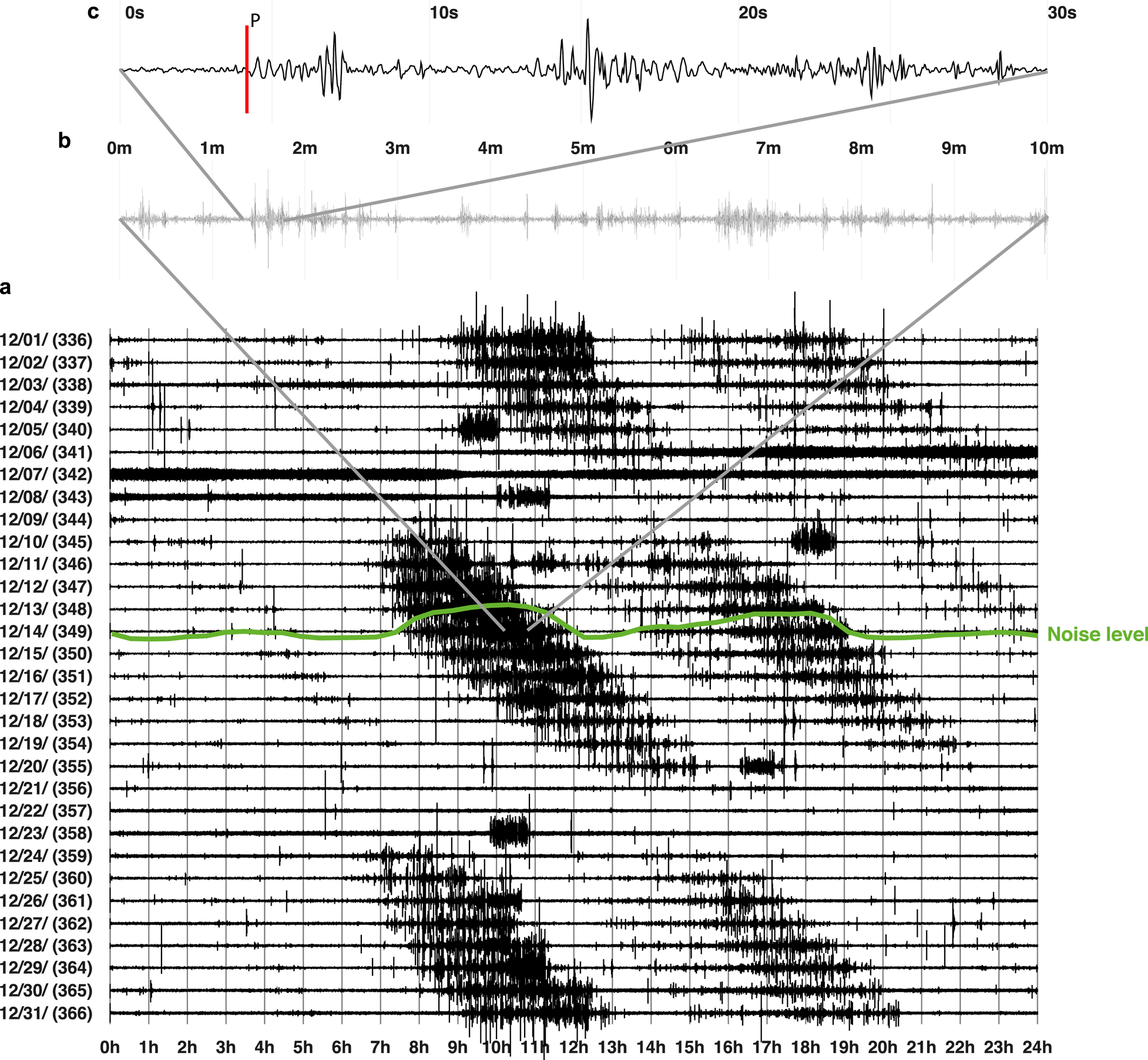
Fig. 2. Helicorder seismogram shows the tidal influence on the seismological record filtered in the range 2–10 Hz. Diagonal bands of high amplitude, high recurrence icequake activity (panel a) indicate tidal modulation. As described in the text, the noise level reflects the higher seismicity (panel b) showcased with the green line for the 14th of December (d 349). The event with the marked P arrival is further analyzed in Fig. 3 (uppermost panel c). Furthermore, storms (e.g. d 341–343) or human activity close to the seismometer highly increase noise levels (d 358 10 h–11 h).
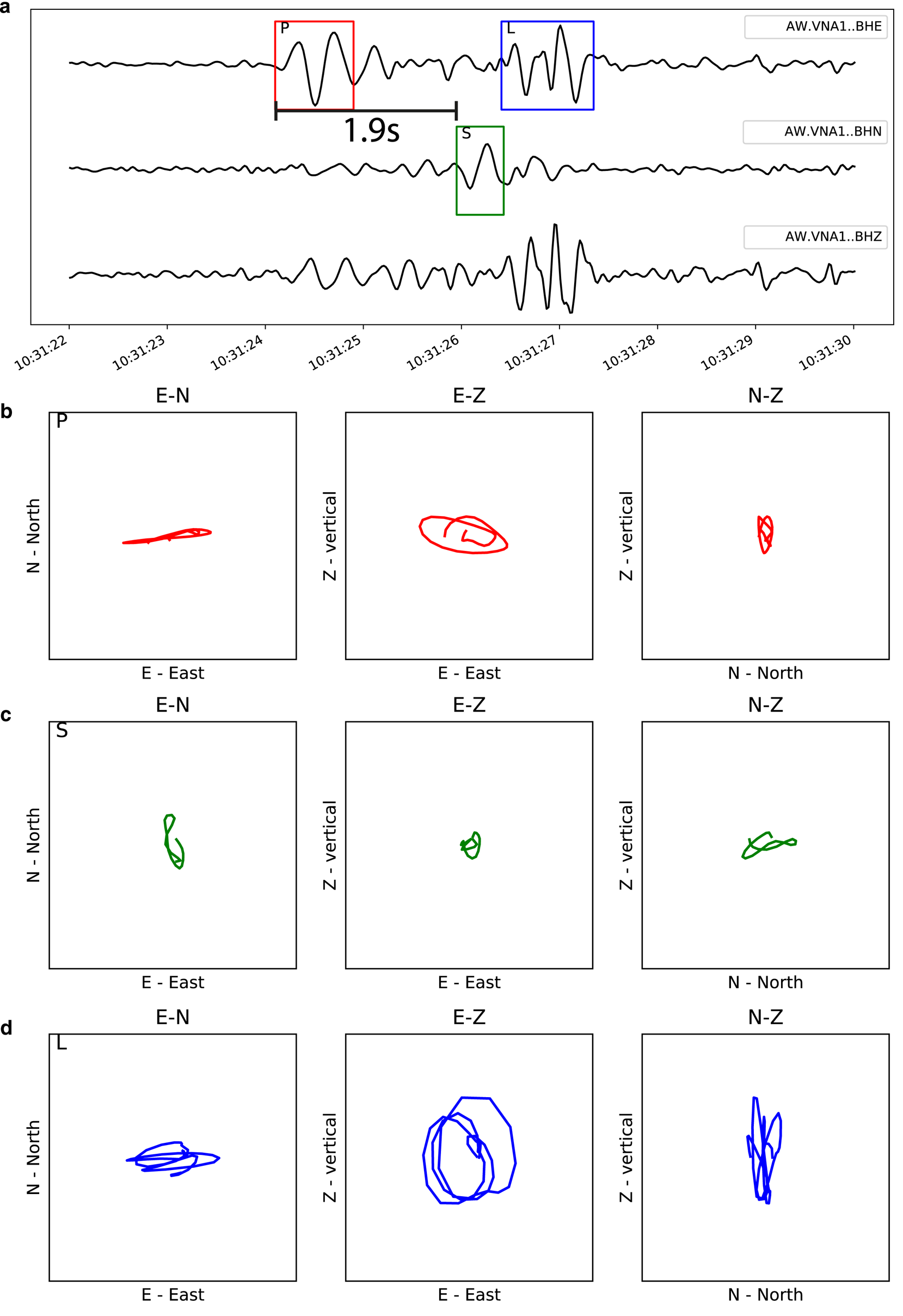
Fig. 3. Waveforms (a) of the three seismometer components for a selected event. The rectangles in panel (a) mark the time windows used for particle motions in panels (b–d) for P, S phases and surface waves (L).
Individual events can clearly be distinguished, but instead of counting the number of events as in previous studies of icequake–tide relations (Barruol and others, Reference Barruol2013; Hammer and others, Reference Hammer, Ohrnberger and Schlindwein2015), we quantified the seismic activity by calculating the probabilistic power spectral densities (PPSD) following procedures described by McNamara and Buland (Reference McNamara and Buland2004) and implemented in the ObsPy Python framework for processing seismological data (Beyreuther and others, Reference Beyreuther2010). We cut the data into 1 h segments with 50% overlap and each hour segment into 13 segments with 75% overlap. We tapered each of these segments and calculated an FFT. Finally, we removed the instrument response and calculated hourly spectral averages for the 13 segments. The spectral densities were then binned into 1/8 octave periods and 1 dB power intervals and probabilities were calculated to produce PPSDs. We then extracted the PPSDs in the frequency bin 3.4–6.8 Hz for each hour-long segment in order to obtain a time series of the seismic noise level around 5 Hz, the frequency range that covers the recorded icequake activities (Fig. 4). Afterward we performed a standard tidal analysis of the seismic noise time series with T_TIDE (Pawlowicz and others, Reference Pawlowicz, Beardsley and Lentz2002), which is based on Foreman (Reference Foreman1978). T_TIDE uses defined frequencies with a rational basis in tidal theory to model a given time series. To ensure that our results are not biased by forcing the frequency content, we also performed a standard FFT confirming the T_TIDE results (Fig. S1, upper panel). For identifying the tidal harmonics and the respective amplitudes we use the T_TIDE results.

Fig. 4. Comparison of vertical displacement from GNSS data, CATS2008 (Howard and others, Reference Howard, Erofeeva and Padman2019) and the time series of noise level (PPSD values) in the frequency bin of 3.4–6.8 Hz for seismometer station VNA1. High wind speeds during a storm between 6th and 9th of December obscure the tidal effects on noise levels and might cause the difference between the GNSS data and the tidal model as a result of a barometric effect.
GNSS dataset
For this study, we analyzed the GNSS data that were recorded in the same year as the seismological data but only covering the months March to December (314.8 d). The GNSS data were recorded with 1 Hz sampling rate with a Novatel PwrPak7 dual frequency GPS/GLONASS receiver, equipped with a Tallysman VeraPhase6000 antenna mounted on the roof of Neumayer Station III. We post processed the data with the kinematic precise point positioning method using the commercial software package Waypoint 8.4 (Zumberge and others, Reference Zumberge, Heflin, Jefferson, Watkins and Webb1997). The data are recorded in day files; therefore jumps might occur between the day solutions. To prevent those jumps we merged three successive day files prior to processing and therefore obtain full day overlaps between the different solutions. In a second step, we combined the 3 d solutions using relative point to point distances in the middle of each 1 d overlap to avoid edge effects.
We smoothed the data with a 3 h wide Gaussian filter and resampled to 10 min sample interval (Fig. 5). When selecting the filter width we balanced spatial GNSS and frequency resolution. The Ekström Ice Shelf moves with ~1.76 cm h−1, which is a small displacement to measure with a single-GNSS station without a nearby reference station. At the same time, the time windows must not exceed half of the signal wavelength of interest, which is 6 h or 4 cpd. We therefore chose the widest possible window without suppressing the HF signals. However, the characteristics of the Gaussian filter removes some energy from the 3 and 4 cpd signals and substantially reduces signals higher than 5 cpd. Next, we calculated displacement and velocity and applied the T_TIDE analysis. As with the seismic noise data we calculated an unbiased FFT spectrum for the ice velocity (Fig. S1, lower panel).
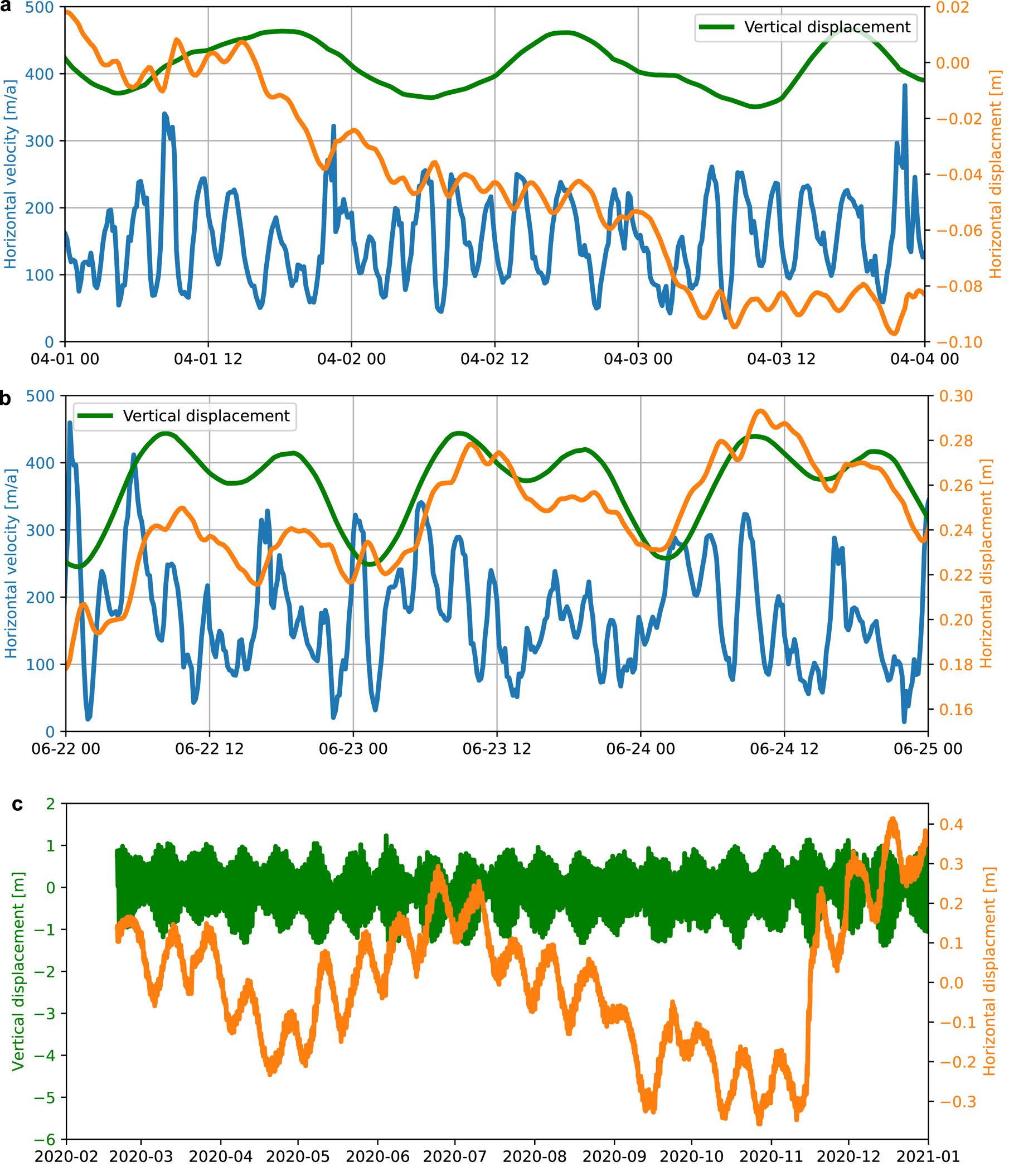
Fig. 5. Displacement and velocity derived from GNSS data for 3 d during a predominantly diurnal neap tide period (a), a semi-diurnal spring tide period (b) and for the full year (c). The displacement is detrended with the yearly mean displacement. The scale for the vertical displacement is the same for (a) and (b). During the neap tide (a) the displacement reveals a ‘steppy’ behavior, like a weak stick–slip situation, which is absent in the spring tide period (b). Here, the displacement shows a semidiurnal periodicity similar to the vertical displacement. Over the whole year, fortnightly periodicity dominate the displacement (c).
Observations
The processed data reveal tide-dependent seismic noise level variations in the frequency band between 3.4 and 6.8 Hz (Fig. 2). Large numbers of cryogenic events cause peaks in seismic noise level. Single events originate typically in 5–10 km distance, estimated from S–P travel time differences of 1.5–2.0 s (Fig. 3a) in an east–west direction (Fig. 3b). Based on these constraints, the potential source area for the events is an ice shear zone and grounding zone at one of the foothills of the Atkakuppelen ice rise, which lie ~6 km east of VNA1 (Fig. 1). To further investigate the source mechanism, seismic stations have been deployed along the shear zone and results will be published elsewhere.
The seismic noise level spectrum shows the main semi-diurnal (M2, S2 and K2) and diurnal (O1, K1) tidal periodicities, but also strong spectral components of the HF tides with ~3 cpd and ~4 cpd periodicities (Fig. 6a and the unbiased FFT in Fig. S1a, Table 1). The spectral amplitudes of the 4 cpd tides are the largest HF component and as large as the diurnal tides (~1 cpd). Next, the 3 cpd components are larger than the main semi-diurnal components (~2 cpd). Both higher-harmonic period bands split up into separate peaks, with major roles of the compound tides MS4, M4, SN4 and MK3, SO3, M3, MO3 (the full report and the tidal analysis is part of the Supplementary material, listing1).
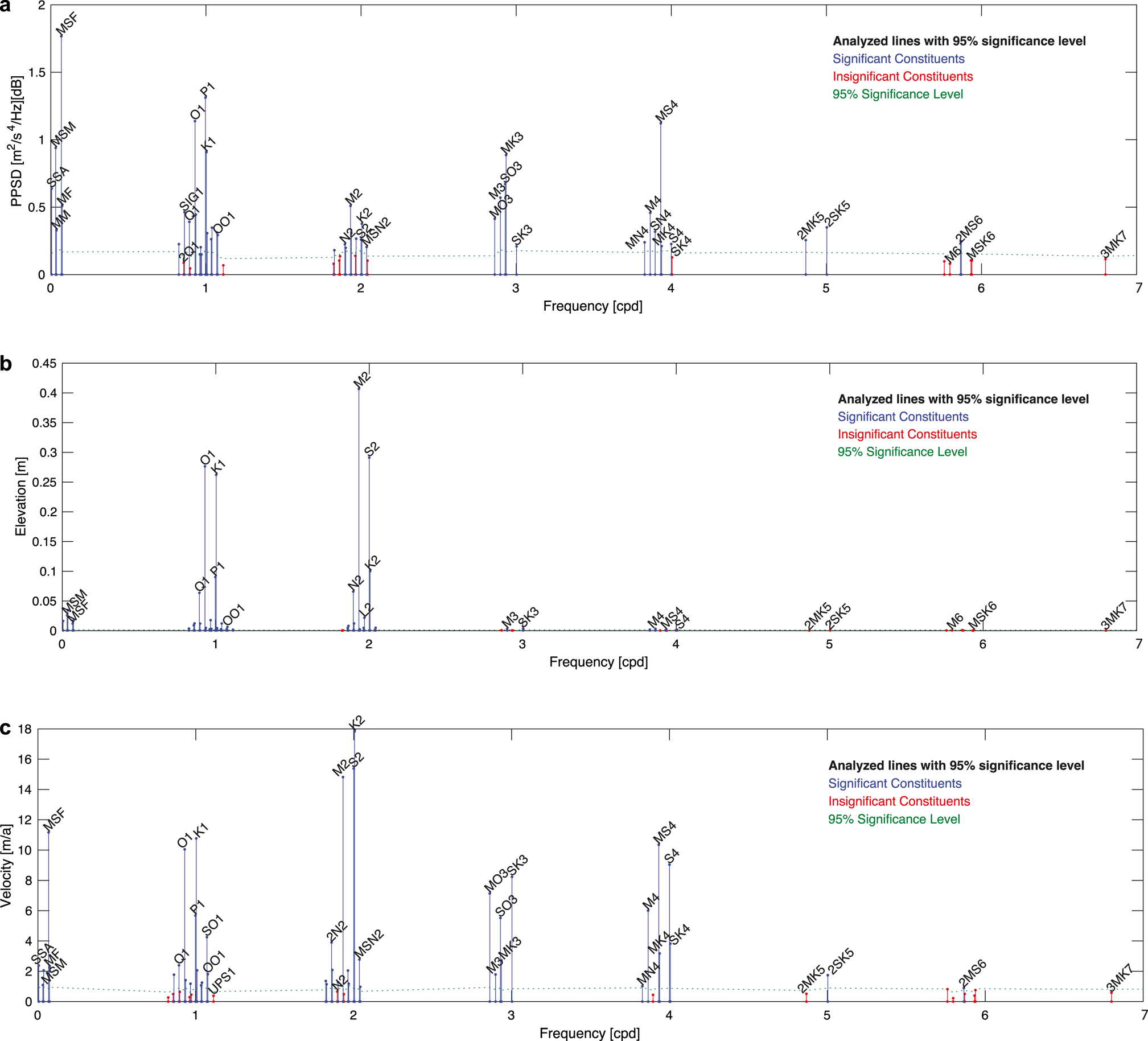
Fig. 6. Spectral analysis of (a) seismic noise levels, (b) vertical GNSS and (c) horizontal ice flow velocity. Seismic noise levels (a) and the vertical GNSS component (b) show the main tidal constituents O1, K1, M2, S2 in the 1 and 2 cpd band. Additional higher tidal constituents of in the 3 and 4 cpd band (e.g. MK3, MS4) are clearly visible in seismic noise (a) and ice flow velocity (c), but not in the vertical displacement (b). This suggests that horizontal velocity modulations affect the icequake activity in the HF band more than vertical shelf movements. For clarity, only labels of selected constituents are shown. Exact amplitudes on all partial constituents are reported in the Supplementary listings 1–3. Note, that signals in the GNSS data with 3 and 4 cpd are damped by the 3 h Gaussian filter and signals higher than 5 cpd substantially reduced (only GNSS data).
Table 1. Main tidal constituents and their corresponding periods measured at the Ekström Ice Shelf using different instrumentation
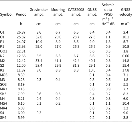
Kobarg (Reference Kobarg1988) derived tidal amplitudes from a gravimeter, Tezkan and Yaramanci (Reference Tezkan and Yaramanci1993) from a mooring in Atka bay. MS4, SO3 and MK3 are clearly visible in the seismological data and in the ice velocity, but have not been observed in vertical tidal amplitudes. The full results for GNSS and seismic data are shown in the Supplementary listings 1–3.
The strongest component in the seismic noise spectrum is the lunisolar synodic fortnightly MSF, which also dominates the horizontal displacement data over the course of the year (Fig. 5c). Also, all the other components vary in strength over the course of the year with fortnightly and possible seasonal variation (Fig. 7). We find larger amplitudes during spring tides than neap tides and some longer-term variation with nearly no terdiurnal occurrence during fall (March) and strongest amplitudes in June/July. This finding is in agreement with observations made at the Rutford Ice Stream (Aðalgeirsdóttir and others, Reference Aðalgeirsdóttir2008).

Fig. 7. Spectrogram of the PPSD noise values in comparison with tidal amplitudes from the CATS2008 model (Howard and others, Reference Howard, Erofeeva and Padman2019). The spectrogram was calculated with a time window of 10.6 d and an overlap of 9.6 d. Note, that a spectrogram shows the band-integrated energy as a function of time and therefore the individual harmonics are no longer resolved. The amplitudes of the tidal constituents in the noise change depending on the tidal range and are generally larger during spring tides than neap tides.
The observed vertical amplitudes associated with the major harmonics measured with GNSS data generally match well with those in previous measurements from the 1980s and 1990s (Kobarg, Reference Kobarg1988; Tezkan and Yaramanci, Reference Tezkan and Yaramanci1993) and the CATS2008 model (Howard and others, Reference Howard, Erofeeva and Padman2019), an update to the model described by Padman and others (Reference Padman, Fricker, Coleman, Howard and Erofeeva2002). However, the magnitude of the GNSS measured spectral amplitudes differs from the seismic noise spectra (Table 1, Figs 6a, b). As expected, the vertical amplitudes are dominated by the major diurnal and semi-diurnal harmonics. The most energetic harmonics are M2 (~41 cm) followed by S2 (~29 cm), O1 (~28 cm) and K1 (~26 cm). As in the seismic data, we can also trace HF tides, but amplitudes are 100 times less than the dominant M2 harmonic with maximum amplitudes of 0.31–0.37 cm for M3 to SK3 (Supplementary listing 2).
Similarly to the seismic noise data, the GNSS derived ice velocity periodically varies with the tides. The average ice shelf velocity is 154 m a−1 with a std dev. of 75 m a−1 ranging mostly between 79 to 229 m a−1 (Fig. 5b). The tidal analysis reveals the full spectrum of tidal constituents and contains strong ~3 and ~4 cpd components (Fig. 6c). The dominant amplitudes are the semi-diurnal tides at K2, S2 and M2 followed by the fortnightly MSF, the diurnal tides and the quarter- and terdiurnal components, all in the same order of magnitude. As for the seismic data, the ~4 and ~3 cpd components split up in separate peaks with the similar harmonics MS4, S4, M4, SK4, MK4 and SK3, MO3, SO3, MK3 and M3 (Supplementary listing 3, Fig. S1b).
Comparing the different spectra, we see that the dominant effects of the signals with ~4 and ~3 cpd frequencies, which correspond to HF tides are evident in both: seismic noise levels and GNSS-derived horizontal ice motion. In contrast, the vertical tidal components, with amplitudes of ~0.3 cm are far smaller than the 29–41 cm associated with the semidiurnal tides (Fig. 6b), while the seismic noise variations associated with the HF tides exceed those associated with the semidiurnal ones (Fig. 6a, Table 1).
Interpretation and discussion
HF tides appear due to the presence of non-linear processes. It is not surprising that the vertical displacement spectrum does not show a pronounced role of HF tides (Fig. 6b and Supplementary listing 2), because there are no significant sources of non-linearity in the area of GNSS measurements. The elevation is dominated by the major harmonics both in observations and modeling results. However, in shallow areas near the grounding zone non-linear effects may occur through many possible mechanisms from ocean (e.g. friction between water layer and bed/ice) and non-ocean (e.g. anelastic ice deformation) sides (Pedley and others, Reference Pedley, Paren and Potter1986). The problem here is that we cannot distinguish and weigh the contributions from different non-linear terms. Below we discuss in detail possible causes and related mechanisms for tide induced icequake activity: vertical tidal movement and horizontal tidally induced movement of ice shelf. Indeed, it is clear that they are ultimately related.
Vertical tidal movement as icequake source
Vertical tidal movement has several distinct effects on ice quake activity. During tidal cycles, icequakes can occur near the grounding zones of ice shelves by crevassing at the ice surface and base (Barruol and others, Reference Barruol2013; Hammer and others, Reference Hammer, Ohrnberger and Schlindwein2015; Hulbe and others, Reference Hulbe2016). Here, the vertical tidal movement of the floating ice shelf bends the ice, inducing stress at the outer bend that leads to brittle failure where it exceeds the strength of the ice. Hence, the larger the tidal range, the larger the flexure-related icequake activity.
Another source for icequake activity are pinning points with patches of grounded ice. Here, basal seismicity originates from horizontal stick–slip events as the ice shelf moves over bed rumples. Even though the events are caused by horizontal motion, the vertical tidal variations are the primary cause. The vertical displacement of the ice shelf changes the contact area between ice and bedrock and the stress generated at it. Depending on the geometry of the contact area, this kind of seismicity can occur during high or low tides (Osten-Woldenburg, Reference Osten-Woldenburg1990; Pirli and others, Reference Pirli, Hainzl, Schweitzer, Köhler and Dahm2018), e.g. tides could lift the ice, reduce the contact area and, therefore, friction, allowing the ice to move and causing icequakes during high tides. Or a pinning point could lose contact to the ice completely during high tide and basal stick–slip icequakes would occur only during low tide when the ice is ephemerally grounded. Hence, the occurrence of stick–slip events also depends on vertical tidal motion.
The vertical tidal amplitude is the main parameter controlling both stick–slip-related icequakes and flexure-related icequakes. However, the GNSS spectra reveal only little vertical displacement with 3 and 4 cpd (Fig. 6b and Supplementary listing 2). Parts of the quarter-diurnal tidal period might be explained with flexure-related source models. Minowa and others (Reference Minowa, Podolskiy and Sugiyama2019) and Hammer and others (Reference Hammer, Ohrnberger and Schlindwein2015) observed peaks in seismicity during periods of maximum vertical speed, which occur every 6 h during rising and falling semi-diurnal tides and not at high or low tide. For the HF band a vertical tidal movement is nearly absent. However, note that the GNSS data are recorded in the ‘middle’ of the ice shelf, whereas the icequakes occur at the fringe of the shelf near an ice shear zone and a grounding zone. There might be a vertical 3 and 4 cpd tide at the grounding zone large enough to generate flexure driven icequakes either because of anelastic ice deformation (Pedley and others, Reference Pedley, Paren and Potter1986) and/or non-linear ocean-related processes, e.g. friction between water and ice/bed, which cause elevation spectra dominating by HF tides.
Ice velocity modulation as icequake source
In contrast to the vertical displacement data, the ice velocity displays the same high harmonics as the seismic data (Fig. 6). To explain these signals, we consider another potential source of icequake activity, shear fracture, caused by tidal variability of shear. East of Neumayer Station is an ice shear zone, where the ice velocity drops from 154 m a−1 at the Ekström Ice Shelf to 8 m a−1 between the grounded Halvfarryggen and Atkakuppelen (Fig. 1, Rignot, Reference Rignot2017). Instead of vertical tidal motion, changes in this horizontal flow velocity gradient, as the velocity of the floating ice responds to tidal forcing, may control icequake activity by crevassing at the shear margin. Consistent with the seismic noise data, we observe tidal modulations of the ice shelf flow velocity with a large role of variations in the HF signals (Fig. 6c).
In general, tidally forced velocity variations are still not fully understood. The subject is complex and involves various non-linear relationships, for example between basal sliding and sediment deformation (Gudmundsson, Reference Gudmundsson2007) and/or grounding line migration (Rosier and Gudmundsson, Reference Rosier and Gudmundsson2020). Basal sliding is affected by ocean water pumped across the grounding line under the still-grounded ice through sediment till and/or basal channels in the sub-glacial hydrology. This subglacial water might reduce friction and lubricate the ice–rock interface, resulting in increased ice velocities (Sayag and Worster, Reference Sayag and Worster2013), which we observe in our GNSS data (Fig. 8). The inflow area near the grounding zone of ice streams feeding an ice shelf is a sensitive area for velocity modulations, which can be observed far upstream of the grounding line (e.g. Anandakrishnan and others, Reference Anandakrishnan, Voigt, Alley and King2003).
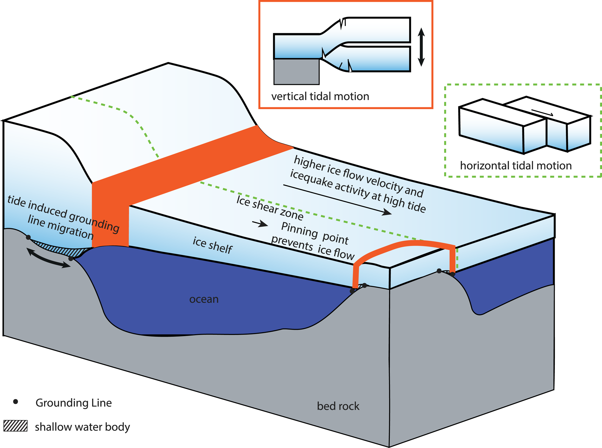
Fig. 8. Sketch of possible icequake sources related to tides. Vertical tidal motion leads to flexure-related cracks in the red areas near grounding zones. Moreover, tidal grounding line migration creates a thin water layer beneath the ice leading to a pronounced role of non-linear processes. The water film leads to higher ice flow velocities and can cause higher icequake activity at shear zones (dashed green line).
The Ekström Ice Shelf is mainly fed by three unnamed ice streams ~100–150 km away from Neumayer Station (Fig. 1, A–C). At ice stream ‘B’, the grounding line migration has been measured by GNSS and gravity measurements and can be inferred from satellite interferometry. Riedel and others (Reference Riedel, Nixdorf, Heinert, Eckstaller and Mayer1999) observed a maximum uplift of 15 cm at a location 1 km upstream of the mean grounding line at the Ekström Ice Shelf. Satellite interferometry indicates that tidal variation causes the location of the grounding line to oscillate by ~1.5–2.5 km (personal communication from Neckel, 2020, Fig. S2). During tidal cycles, a shallow water body forms beneath the ice in the grounding zone. This shallow water body and shallow water at the grounding zone in general might generate HF tides as diurnal and semi-diurnal tides interact in a non-linear way while the signal of the major diurnal and semi-diurnal harmonics become weaker (Pedley and others, Reference Pedley, Paren and Potter1986; King and others, Reference King2011). Heinert and Riedel (Reference Heinert and Riedel2007) observed HF tides and weak semi-/diurnal tides with GNSS and gravimeter measurements upstream of the mean grounding line at ice stream ‘B’: vertical tidal movements with 3 and 4 cpd and amplitudes of 0.35 and 0.6 cm respectively, while diurnal and semi-diurnal components are absent. This indicates that non-linearity from ocean side might play a role in the modulation of horizontal velocities through rectification of oscillatory tidal currents resulting in tidal residual flow (e.g. Robinson, Reference Robinson1983).
The icequake activity is not a linear result of the ice motion. For example, the strongest amplitudes in M2 and S2, both horizontally and vertically, are not matched by an equally strong signal in the seismological signal. How exactly the seismic noise relates to the ice motions cannot be resolved here with our datasets. In general, the seismic spectra are similar to the velocity spectrum. We propose the horizontal ice flow as main source for the periodic icequake activities in the HF bands as the non-linear response of the ice stream to the vertical tidal forcing (Fig. 8).
The effects of HF tides are not limited to the Ekström Ice Shelf. The phenomenon has also been observed at other ice shelves and ice streams. Terdiurnal variations in velocity and seismicity occur, for example, at Rutford Ice Stream (Murray and others, Reference Murray, Smith, King and Weedon2007; Aðalgeirsdóttir and others, Reference Aðalgeirsdóttir2008), Mertz Glacier (Barruol and others, Reference Barruol2013), the Filchner–Ronne-(King and others, Reference King2011) and George-VI-ice shelves (Pedley and others, Reference Pedley, Paren and Potter1986). While Murray and others (Reference Murray, Smith, King and Weedon2007); Aðalgeirsdóttir and others (Reference Aðalgeirsdóttir2008) and Barruol and others (Reference Barruol2013) shortly mentioned the existence of HF signals in their data, King and others (Reference King2011) and Pedley and others (Reference Pedley, Paren and Potter1986) discussed possible origins in detail. Pedley and others (Reference Pedley, Paren and Potter1986) speculated that anelastic ice deformation in the grounding zones might be the source of HF tides. King and others (Reference King2011) noted that only harmonics with 4 cpd increased in amplitude toward the grounding zone at the Filchner–Ronne Ice Shelf in line with Pedley and others (Reference Pedley, Paren and Potter1986) suggestion, but harmonics with 3, 5 and 6 cpd decreased and therefore, are not generated in the grounding zone. The origin of the latter HF tides might be of oceanic (including friction between water layer and ice/bed) or of glaciological origin (pumping effect).
Conclusion
We have observed consistent energy distributions in the spectra of seismic noise and ice velocity data in the HF range that are as large as, or even larger than, those of the main tides. The observed icequake activity is likely caused by shear fractures related to the gradient in horizontal ice shelf motion near the fringes of the ice stream, where the ice flow speed drops to nearly zero. We hypothesize that the grounding zone of the ice stream feeding the ice shelf is the origin of the velocity variation. Here, friction and other sources of non-linearity might cause the appearance of HF tidal signals in ice velocity, consequently leading to shear failure of the ice. Further studies are necessary to constrain the exact focal mechanism of the icequakes, which would allow us to identify the origin of the icequakes (shear or flexure) and, consequently, the underlying processes. For such studies, seismic networks around the potential source regions are needed. Additional studies with GNSS and seismic data at the ice streams feeding the shelf can potentially shed light on the origins of the velocity variations. However, even without such large experiments a single-seismic station adjoined by a GNSS receiver reveals new insights into the tidal impact on ice dynamics. As it is shown here, the tidal impact is much more dynamic than previously thought with tidal constituents that are often not considered. We should regularly consider tidal HF signals in GNSS, seismic and oceanographic data and models in future studies. Tide-influenced processes like mass balance and mean flow velocity might be more pronounced when resolving HF signals in the models than currently considered. Understanding tide-related ice dynamics is important for predicting future ice dynamics in the light of a changing environment with changing sea level and ice conditions and therefore, changing tidal dynamics.
Supplementary material
The supplementary material for this article can be found at https://doi.org/10.1017/jog.2023.4
Acknowledgements
We thank the winterers, technical and logistical departments at Neumayer Station III for their continuous efforts to keep the observatory operational throughout the Antarctic winters (Wesche and others, Reference Wesche2016). We also thank Erik Buchta, Lutz Eberlein and Abbas Khan for fruitful discussions on our GNSS data and Graeme Eagles for his editing. We are also grateful to the reviewers, who provided constructive feedback.


 Open access