


Impact Statement
Machine learning (ML) models learn from data. To compare and improve ML methods and models, data scientists need standard data sets as benchmark. There exist many standard data sets, like a collection of handwritten digits or images. Our contribution adds a consistent and comprehensive collection of climate indices as new benchmark data set. This collection can be used to train ML models to understand the complex short-term and long-term variability of the climate system and to predict climate events.
1. Introduction
To develop and compare machine learning (ML) methods and models in an objective way, there exist standard data sets as benchmark. Among these data sets, we find, for example, a collection of handwritten digits provided by the National Institute of Standards and Technology, referred to as MNIST data set (Lecun et al., Reference Lecun, Botou, Bengio and Haffner1998). Other data sets contain images, like the CIFAR-10 data set from Canadian Institute for Advanced Research, introduced by Krizhevsky (Reference Krizhevsky2009), or CelebSET, as a collection of photos of celebrities with different ethnicity (Raji et al., Reference Raji, Gebru, Mitchell, Buolamwini, Lee and Denton2020). These data sets are mostly suitable for classification algorithms. Famous data sets for pattern recognition and clustering applications are, for example, Palmer Penguins or the Wine data set, provided by Horst et al. (Reference Horst, Hill and Gorman2020) and the UCI Machine Learning Repository (Murphy and Aha, Reference Murphy and Aha1994), containing attributes for various species of penguins and results of a chemical analysis of wines, respectively. Furthermore, the data science community also provides standard time series collections, for example, the Rainforest Automation Energy data set that contains energy consumption time series for various household appliances (Makonin et al., Reference Makonin, Wang and Tumpach2018). However, benchmark data sets in the field of climate science are rare. To name a few, Mamalakis et al. (Reference Mamalakis, Ebert-Uphoff and Barnes2022) provide a framework to create synthetic data sets designed for problems in geosciences. And Watson-Parris et al. (Reference Watson-Parris, Rao, Olivié, Seland, Nowack, Camps-Valls, Stier, Bouabid, Dewey, Fons, Gonzalez, Harder, Jeggle, Lenhardt, Manshausen, Novitasari, Ricard and and Roesch2022) introduced ClimateBench, as a benchmark for data-driven climate projections.
Here, we are interested in describing the underlying dynamics of the Earth System. Real-world data in this context are limited to observable features that can be measured in a comprehensive way or that can be reconstructed from sparse measurements. Examples are sea surface temperature (SST), sea level pressure (SLP), surface air temperature (SAT), sea surface salinity (SSS), geopotential height at various pressure levels, for example, at 500 millibar (Z500), or total precipitation (PREC). These variables reflect some of the main dynamics of the Earth system in form of known modes of climate variability, patterns, and oscillations, for example, Atlantic Multidecadal Oscillation (AMO) (Schlesinger and Ramankutty, Reference Schlesinger and Ramankutty1994), the Southern Annular Mode (SAM) (Gong and Wang, Reference Gong and Wang1999), or the El Niño Southern Oscillation (ENSO) (Philander, Reference Philander1989). To describe the Earth System dynamics in a compressed way, multi-dimensional physical fields can be reduced to specific climate indices that capture the main processes. For instance, ENSO is a complex phenomenon that can be detected as periodic SST fluctuations in the Tropical Pacific. Several indices are defined to compute the current ENSO phase from area-averaged SST anomalies (SSTA) in certain regions. For instance, the Niño 3.4 index defined from the Niño 3.4 region (5°N–5°S, 120°W–170°W) by the National Oceanic and Atmospheric Administration (NOAA) is often used in the context of ENSO (Climate Diagnostics Bulletin, n.d.). While ENSO is a large-scale driver of the climate system, other indices aim to capture regional variability in specific features, like the Sahel precipitation index (SPI) (Badr et al., Reference Badr, Zaitchik and Guikema2014). This index measures anomalies of summer rainfall in the African Sahel region (10°N–20°N, 20°W–10°E). Real-world climate data are, for example, provided by the Joint Institute for the Study of the Atmosphere and Ocean (n.d.) or National Oceanic and Atmospheric Administration (NOAA) (n.d.). However, climate indices are limited in their temporal extent, since consistent real-world measurements started only in recent history or measurements are subject of specific research projects that run over a certain period in time.
Our aim is to better understand existing modes of climate variability and to find new relationships. Therefore, we require a consistent and comprehensive collection of climate indices over a sufficiently long time span, which favors the use of model data over real-world data. Earth System Models (ESMs) aim to simulate processes of the Earth system in specified temporal and spatial resolution. The Flexible Ocean and Climate Infrastructure (FOCI) (Matthes et al., Reference Matthes, Biastoch, Wahl, Harlaß, Martin, Brücher, Drews, Ehlert, Getzlaff, Krüger, Rath, Scheinert, Schwarzkopf, Bayr, Schmidt and Park2020) and the Whole Atmosphere Community Climate Model (WACCM) as extension of the Community Earth System Model (CESM) (Hurrell et al., Reference Hurrell, Holland, Gent, Ghan, Kay, Kushner, Lamarque, Large, Lawrence, Lindsay, Lipscomb, Long, Mahowald, Marsh, Neale, Rasch, Vavrus, Vertenstein, Bader, Collins, Hack, Kiehl and Marshall2013; Marsh et al., Reference Marsh, Mills, Kinnison, Lamarque, Calvo and Polvani2013) are both coupled, global climate models that provide state-of-the-art computer simulations of the past, present and future states of the Earth system. The quality of model outputs is evaluated on certain control runs. This can, for example, be done by starting an ESM with pre-industrial conditions from the year 1850 and letting the model unfold its dynamics without external forcing over a desired time span. Here, we use the output of FOCI and CESM control runs. In particular, we work with SST, SAT, SLP, Z500, SSS, and PREC as two-dimensional fields. From these variables, we derive a set of climate indices over 1000 and 999 years, respectively. The obtained collection of climate indices based on model data (CICMoD) serves as a reduced description of the Earth system in a consistent and comprehensive way. Our main contributions are as follows:
-
• We introduce CICMoD as a new benchmark data set to the data science community, describing the climate system.
-
• CICMoD allows the user to develop new ML methods and to compare results to existing methods and models in an objective way.
-
• We provide an open-source framework that can be extended and customized to individual needs, for example, by including further ESMs.
-
• Additionally, we briefly sketch two examples of how our CICMoD data set can be used.
Relationships in the climate systems are often characterized as nonlinear and nonstationary (Pak et al., Reference Pak, Park, Vivier, Kwon and Chang2014, Reference Park, Kim, Pak, Yamamoto, Vivier and Durand2018; Zhang et al., Reference Zhang, Mei, Geng, Turner and Jin2019). ML and deep learning (DL) models have been shown to be useful for this kind of problems, for example, by Mayer and Barnes (Reference Mayer and Barnes2021) or Pegion et al. (Reference Pegion, Becker and Kirtman2022). However, working with benchmark data sets bears the risk of having undetected errors and biases or of being unrepresentative. For instance, Liao et al. (Reference Liao, Taori, Raji and Schmidt2021) and Luccioni and Rolnick (Reference Luccioni and Rolnick2022) argue that the ubiquity of benchmarks in computer science has led to efforts that chase benchmark performance at the expense of real-world applications. Thus, once we find new relationships in the Earth System, these findings need to be confirmed on real-world data to identify artifacts in ESM simulations. A better understanding of causally linked modes within our climate system is essential to tackle climate change and to attenuate its impacts.
The rest of this work is structured as follows. In Section 2, we provide a short description of FOCI and CESM. An overview of all indices included in the CICMoD data set and details on how the indices are derived from raw ESM outputs are given in Section 3. In Section 4, we show two exemplary applications and use climate indices from CICMoD data set to predict Sahel rainfall and ENSO, respectively. A detailed discussion of all results and a conclusion is found in Section 5.
2. Model Data
The climate indices included in our CICMoD data set are derived from monthly averaged output of climate model simulations with FOCI and CESM, respectively. The CESM simulation is based on version 1.0.6 with WACCM version 4 (Drews et al., Reference Drews, Huo, Matthes, Kodera and Kruschke2022). The FOCI simulation used in this manuscript is the control simulation referred to as “FOCI-piCtl” based on FOCI version 1.3.0 (Matthes et al., Reference Matthes, Biastoch, Wahl, Harlaß, Martin, Brücher, Drews, Ehlert, Getzlaff, Krüger, Rath, Scheinert, Schwarzkopf, Bayr, Schmidt and Park2020). Both simulations were run using pre-industrial external forcing that is representative for the year 1850. The FOCI pre-industrial control simulation has been initialized from an ocean at rest with a salinity and temperature distribution based on observations approximately from the last 30 years and then ran for 1500 years. Here, we only use the latter 1000 years and skip the first 500 years to allow the model to find its equilibrium. The CESM control simulation has been initialized from another multi-centennial pre-industrial control run provided by the core development team of the National Center for Atmospheric Research (NCAR) (National Center for Atmospheric Research, n.d.) and is therefore already in equilibrium. FOCI (1.8° × 1.8°, 95 vertical levels) and CESM (1.8° × 2.5°, 106 vertical levels) were run at similar horizontal and vertical resolution, although the vertical distribution of the model layers differs significantly between FOCI and CESM. Both models have been extensively evaluated and used in various climate studies. FOCI and CESM are based on very different component models (see Hurrell et al., Reference Hurrell, Holland, Gent, Ghan, Kay, Kushner, Lamarque, Large, Lawrence, Lindsay, Lipscomb, Long, Mahowald, Marsh, Neale, Rasch, Vavrus, Vertenstein, Bader, Collins, Hack, Kiehl and Marshall2013; Marsh et al., Reference Marsh, Mills, Kinnison, Lamarque, Calvo and Polvani2013; Matthes et al., Reference Matthes, Biastoch, Wahl, Harlaß, Martin, Brücher, Drews, Ehlert, Getzlaff, Krüger, Rath, Scheinert, Schwarzkopf, Bayr, Schmidt and Park2020, for details) with different strengths and weaknesses in simulating various aspects of the global climate.
From both control simulations’ output we use Z500, SLP, SST, SSS, SAT, and PREC. All features except SSS are provided on a two-dimensional atmospheric latitude–longitude grid. As SSS was originally stored on the curvilinear ocean grids, it was sampled to the grid of the other atmospheric fields of the respective model by aggregation with xhistogram (Abernathey et al., Reference Abernathey, Squire, Nicholas, Bourbeau, Spring, Bell and Bailey2022). Note, that SAT refers to the temperature in 2 m height for both, CESM and FOCI data.
3. Climate Index Collection
In this section, we give an overview of all indices included in the CICMoD data set and reveal details on how the indices are derived. In total, our CICMoD data set consists of 29 climate indices. The indices can be grouped by the underlying feature. Each feature is discussed separately in the following subsections. We conclude this section with remarks on statistics and pairwise correlation of all indices.
3.1. Geopotential height
Geopotential height is a vertical coordinate with reference to Earth’s mean sea level. Its contours are used to calculate the geostrophic wind which is of interest for climate dynamics. Here, we choose geopotential height at constant pressure of 500 millibar, referred to as Z500. According to NOAA, Z500 relates to winds in the range between 5000 and 6000 meters above mean sea level (National Oceanic and Atmospheric Administration’s National Weather Service, n.d.). We use Z500 to compute the SAM index which relates to the principal mode of variability in the Southern Hemisphere (SH) extratropics. The SAM index can be obtained as the Principle Component (PC) time series of the leading Empirical Orthogonal Function (EOF) of monthly geopotential height anomalies over parts of the SH (20°S–90°S) (Thompson and Wallace, Reference Thompson and Wallace2000). SAM has large impact on climate dynamics of the SH, including Australian rainfall and Antarctic surface temperatures (Marshall, Reference Marshall2007).
3.2. Sea level pressure
SLP refers to the air pressure at sea level. Several indices are derived from SLP and its anomalies. Opposed to the PC-based version described in Section 3.1, the SAM index was originally defined by Gong and Wang (Reference Gong and Wang1999) as the difference of normalized monthly zonal mean SLP at 40°S and 65°S, respectively. Both versions are included in our CICMoD data set.
The Southern Oscillation Index (SOI) is defined as normalized SLP differences between Tahiti (17°41′S, 149°27′W) and Darwin, Australia (12°27′S, 130°50′E) (Walker and Bliss, Reference Walker and Bliss1932). It is used as a measure of the large-scale fluctuations in the air pressure between the Western and Eastern Tropical Pacific and is closely related to ENSO. Similar to SOI, the North Atlantic Oscillation (NAO) index can be computed from SLP as the normalized difference between Reykjavik (64°9′N, 21°56′W) and Ponta Delgada (37°45′N, 25°40′W) (Hurrell, Reference Hurrell1995). Additionally, the NAO index can be obtained as the PC time series of the leading EOF of monthly SLP anomalies over the Atlantic sector (20°N–80°N, 90°W–40°E) (National Center for Atmospheric Research, n.d.). The NAO refers to swings in the atmospheric SLP between the Arctic and the subtropical Atlantic that are associated with changes in the mean wind speed and direction. Such changes are reflected in the seasonal mean heat and moisture transport between the Atlantic and the neighboring continents and have an impact on the intensity and number of storms, their paths, and their weather (Hurrell et al., Reference Hurrell, Kushnir, Ottersen and Visbeck2003).
The North Pacific (NP) index measures interannual to decadal variations in the atmospheric circulation. It is derived from area-weighted SLP anomalies in a box bordered by 30°N to 65°N and 160°E to 140°W (Trenberth and Hurrell, Reference Trenberth and Hurrell1994). Each grid point’s SLP anomaly value represents the mean value over the corresponding grid box. Since the area of the grid boxes depends on the latitude, we need to use area-weighted SLP anomalies to avoid overestimating values in high latitudes. Usually, the index focuses on anomalies during November and March. Here we keep full information and provide monthly anomalies for all months of a year.
3.3. Sea surface temperature
SST is the ocean temperature close to the surface. By removing the seasonal cycle, we obtain SST anomalies (SSTA). In particular, we subtract the mean over time separately for each month. SSTA impact the energy transfer at the interface between ocean and atmosphere and are of high interest for describing processes in the climate system. Several modes of variability are known to exist on different time scales in the range of years, decades, or even longer. AMO refers to a natural variability occurring in the SST of the North Atlantic with a multidecadal period of 60–80 years. AMO is computed from area-weighted SSTA of the North Atlantic (Trenberth and Shea, Reference Trenberth and Shea2006).
The Pacific Decadal Oscillation (PDO) index is obtained as the PC time series of the leading EOF of monthly SSTA in the North Pacific basin (20°N–60°N, 120°E–260°E). PDO resembles ENSO in its spatial pattern. However, ENSO is referred to as an interannual phenomenon while PDO is decadal in scale (Newman et al., Reference Newman, Alexander, Ault, Cobb, Deser, Di Lorenzo, Mantua, Miller, Minobe, Nakamura, Schneider, Vimont, Phillips, Scott and Smith2016).
ENSO is characterized by periodic fluctuations in SST in the Tropical Pacific. Its positive and negative phases relate to unusual warm (El Niño) or cold (La Niña) SST, respectively. Tropical Pacific is divided into specific regions, so-called Niño regions. ENSO indices are then derived from SSTA in the corresponding region by spatial averaging. Indices are divided by the standard deviation of area-weighted SST over time in the same region, as normalization. Here, we include Niño 1 + 2 region as the smallest and eastern-most Niño region where the phenomenon was first recognized by the local coastal population. Additionally, we present ENSO indices on Niño 3, 3.4, and 4 regions, respectively (National Oceanic and Atmospheric Administration, n.d.). ENSO is a large-scale driver of the climate system (Philander, Reference Philander1989). Usually, ENSO indices are smoothed by taking the rolling mean over several months to erase noise. Here, we omit the rolling mean and provide pure SSTA indices instead, to preserve full information.
Other regions of interest in the context of climate dynamics related to SSTA are Tropical North Atlantic, Tropical South Atlantic, Eastern Subtropical Indian Ocean, Western Subtropical Indian Ocean, Mediterranean Sea, and hurricane main development region, respectively. For instance, the African summer monsoon is found to be highly sensitive to SST variability in all tropical basins (Giannini et al., Reference Giannini, Saravanan and Chang2003). Corresponding indices are included in our CICMoD data set.
3.4. Sea surface salinity
SSS measures the amount of salt dissolved in the ocean surface water and plays an important role in ocean circulation processes. Furthermore, rainfall on land is largely supplied by evaporation over the ocean and that evaporation leaves an imprint in SSS. Here, we include several indices derived from SSS anomalies (SSSA) in specific regions of the Atlantic Ocean introduced by Li et al. (Reference Li, Schmitt, Ummenhofer and Karnauskas2016).
3.5. Surface air temperature
SAT is the air temperature close to the surface and relates to the ability of evaporation, since warmer air has a higher storage capacity for water vapor. Like this, SAT anomalies (SATA) influence the energy transfer at the interface between Earth’s surface and atmosphere. Here, we track area-averaged monthly SATA on large scales with indices covering complete NH and SH (Jones et al., Reference Jones, New, Parker, Martin and Rigor1999). Additionally, we split NH and SH into land-only and ocean-only regions, respectively, and include corresponding indices in our CICMoD data set. The ocean masks are taken from the native model grids.
3.6. Precipitation
Precipitation has a high impact on society in form of extreme events like flooding caused by heavy rainfall or droughts due to missing or lower as normal rainfall. As an example, we include the SPI as measure for rainfall in the African Sahel region (Badr et al., Reference Badr, Zaitchik and Guikema2014). The rainy season in this area is centered on June through October (Joint Institute for the Study of the Atmosphere and Ocean, n.d.). In its original form, the SPI gives a measure of the year to year variability of Sahel rainfall as mean over the rainy season. Moreover, we provide the SPI as monthly anomalies of rainfall in the Sahel zone (10°N–20°N, 20°W–10°E) to preserve full information.
3.7. CICMoD data set
Table 1 gives an overview of all 29 indices included in CICMoD data set ordered by the underlying feature. By definition, all indices have zero mean over time, whereas only NAO_PC, PDO_PC, SAM_PC, SAM_ZM, and SOI are normalized by design to have unit variance. If required, normalization of the remaining indices can be done in pre-processing. Exemplary, pairwise correlation coefficients for all indices included in CICMoD data set derived from FOCI data are shown in Figure 1. Indices derived from CESM data show similar characteristics. ENSO indices are found to be highly correlated, as expected, since these indices are all computed from SSTA in some narrow region of the Tropical Pacific. Additionally, we find station- and PC-based NAO indices to be highly correlated, as well as PC-based SAM and SAM from zonal mean, as these indices are designed to describe the same processes. Indices regarding SATA in the NH and SH, respectively, and indices regarding SSS anomalies in the North Atlantic also reveal similarities in terms of high correlation, since by design spatially related features are involved in the computation. Besides that, SOI is found to be negatively correlated to all ENSO indices. Periods of negative (positive) SOI values coincide with warmer (colder) than normal ocean water across the Eastern Tropical Pacific, which is typical for El Niño (La Niña) episodes (Power and Kociuba, Reference Power and Kociuba2011).
Table 1. All indices are included in CICMoD data set with their acronyms and spatial domains, ordered by the underlying feature.

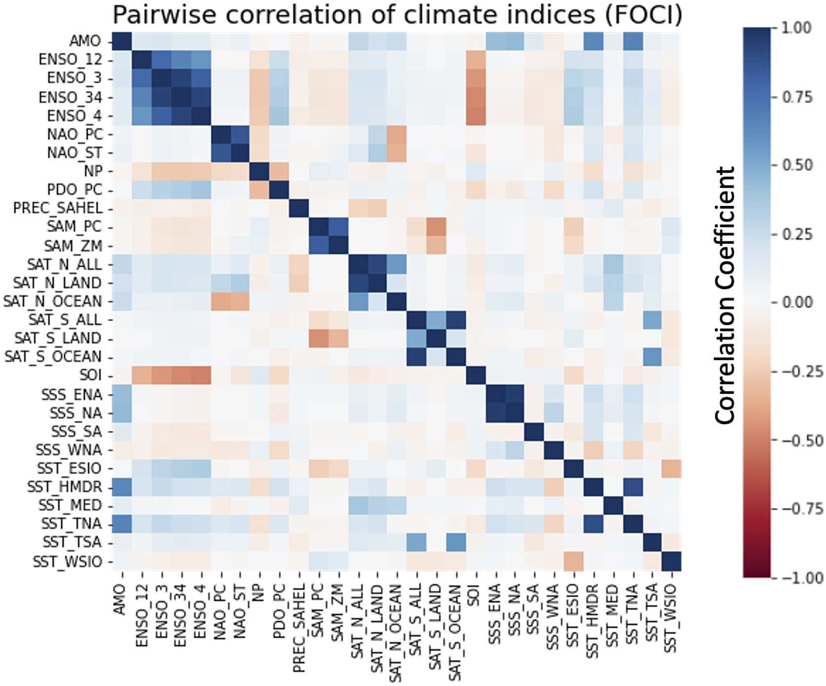
Figure 1. Pairwise correlation coefficients of all CICMoD indices derived from FOCI data.
4. Application and Results
In this section, we briefly sketch two applications of our CICMoD data set to predict Sahel rainfall and ENSO, respectively.
4.1. Sahel rainfall
Sahel summer precipitation has been observed to be highly variable with floods and droughts occurring on a regular basis and has a high impact on living conditions in the region. Predicting Sahel rainfall and understanding the underlying processes is essential, since it allows taking measures in advance to avoid damage and prevent hunger crises. As a first application, we use ML models on our CICMoD data set to predict rainfall in the Sahel region. In particular, we apply a linear regression model as a baseline and, additionally, train a multilayer perceptron (MLP). Following the approach of Badr et al. (Reference Badr, Zaitchik and Guikema2014), we use April to June mean index values for all indices included in our CICMoD data set except SPI as predictors to infer July to September seasonal sum of SPI as target. The input layer of the MLP thus consists of 28 input units. Additionally, we have two hidden layers with 20 and 10 units, respectively, and a single output unit. We use a linear activation function and train the MLP over 10 epochs with a batch size of 10, set the learning rate to
 $ 0.0005 $
and use the Adam optimizer (Kingma and Ba, Reference Kingma and Ba2014). For FOCI and CESM data, the first 800 years are used as training data, while the remaining 200 and 199 years, respectively, are used for validation. Figure 2 shows results from MLP models. Results from linear regression are similar and therefore not shown, here. To evaluate model performance, we look at mean squared error (MSE) of predictions compared to true targets used as objective or loss function. Additionally, the correlation of predicted values and true targets is computed as metric. Corresponding MSE and correlation for linear regression and MLP models on FOCI and CESM data, respectively, are shown in Table 2.
$ 0.0005 $
and use the Adam optimizer (Kingma and Ba, Reference Kingma and Ba2014). For FOCI and CESM data, the first 800 years are used as training data, while the remaining 200 and 199 years, respectively, are used for validation. Figure 2 shows results from MLP models. Results from linear regression are similar and therefore not shown, here. To evaluate model performance, we look at mean squared error (MSE) of predictions compared to true targets used as objective or loss function. Additionally, the correlation of predicted values and true targets is computed as metric. Corresponding MSE and correlation for linear regression and MLP models on FOCI and CESM data, respectively, are shown in Table 2.
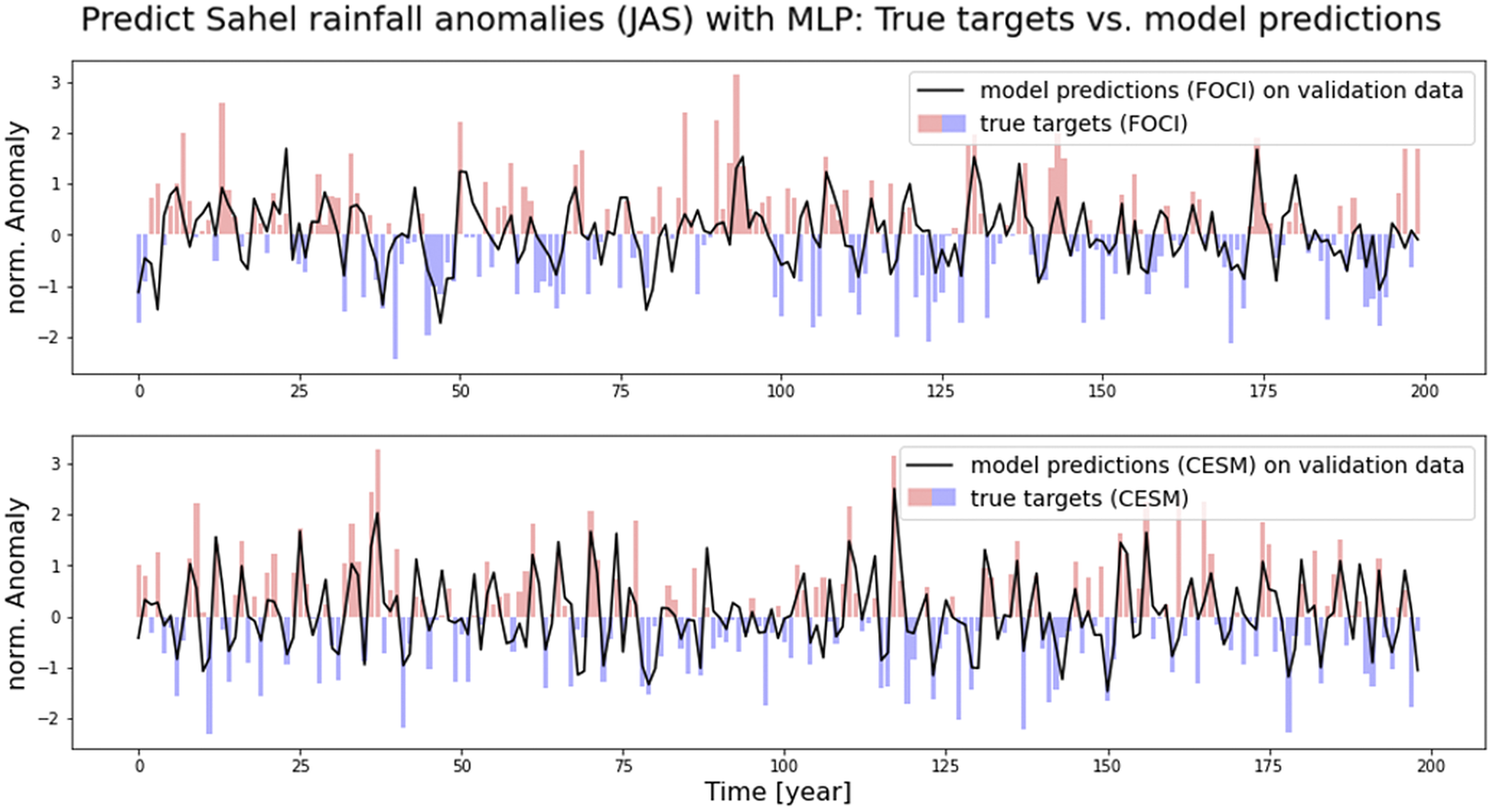
Figure 2. Fidelity check on validation data: Sahel rainfall predictions (black line) from MLP models on FOCI data (upper part) and CESM data (lower part), respectively, compared to true targets shown as a bar plot.
Table 2. Evaluating model performance for predicting Sahel rainfall with linear regression (lin. reg.) and MLP models trained on FOCI and CESM data, respectively.
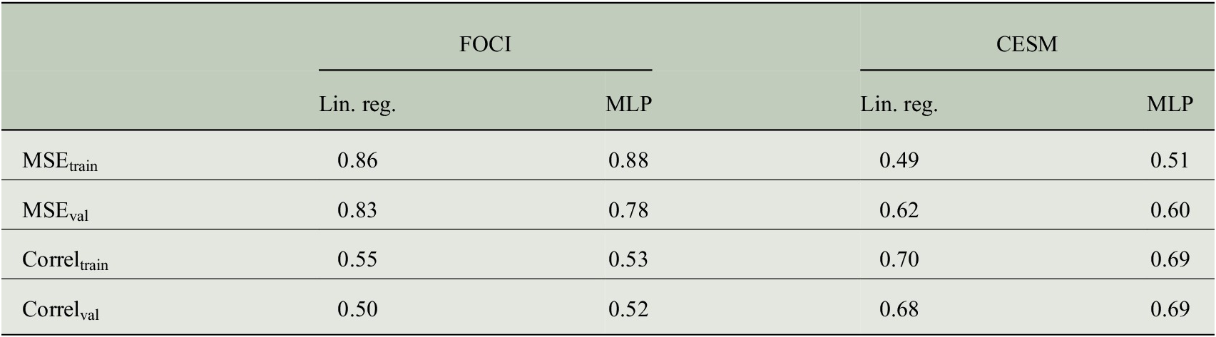
Note. The MSE and correlation (Correl) of predicted values and true targets are shown separately for training and validation data.
4.2. El Niño Southern Oscillation
ENSO is the predominant variation of winds and SST in the Tropical Pacific. The positive phase (El Niño) is characterized by unusual warm SST and high SLP in the Eastern Tropical Pacific, whereas the negative phase (La Niña) relates to unusual cold SST and low SLP in the same region and above-average SST in the Western Tropical Pacific. Both events last several months and occur with a period of 2–7 years with varying intensity per period. ENSO tremendously affects those countries bordering the Pacific Ocean. Strong El Niños, for example, correspond to warm weather conditions with heavy rainfalls from April through October causing major flooding along the West coast of South America near Ecuador and the Northern part of Peru (Cai et al., Reference Cai, McPhaden, Grimm, Rodrigues, Taschetto, Garreaud, Dewitte, Poveda, Ham, Santoso, Ng, Anderson, Wang, Geng, Jo, Marengo, Alves, Osman, Li, Wu, Karamperidou, Takahashi and Vera2020). Consequences of La Niña are, for example, heavy rainfalls over Malaysia, the Philippines, and Indonesia. Therefore, knowing the ENSO phase several months in advance is of high interest for society since it allows to take measures to avoid damage and to protect people. As second example, we use different ANN models on our CICMoD data set to predict ENSO with various lead times. In particular, we train convolutional neural networks (CNNs) and long short-term memory (LSTM) models to predict current ENSO phase and ENSO phase 3 and 6 months into the future, respectively. Here, targets are derived from ENSO_34 time series included in CICMoD, which reflects Niño 3.4 index. As input features, we use all remaining indices from our CICMoD data set, excluding other Niño indices due to the high correlation to our targets. Input features are split into sequences of 24 months. We thus try to predict current and future ENSO phases from past 2 years’ conditions.
In particular, the CNN models are based on two one-dimensional convolutions with 10 and 20 filters, respectively. Kernel size is set to 5 with a stride of 1. Each convolution is followed by batch normalization, a leaky rectified linear unit activation with negative slope coefficient
 $ \alpha =0.3 $
, and a maximum pooling operation with a pool size of 2. The output of the final pooling operation is then flattened and used as input for two fully connected layers with 20 and 10 units, respectively, and finally, we have a single output unit. The LSTM models are based on two LSTM layers with 10 and 20 units, respectively. The output of the final LSTM layer is used as input for two fully connected layers with 20 and 10 units, respectively, and finally, we have a single output unit, similar to the CNN models. Furthermore, we use a linear activation function for all fully connected layers and the output unit and train the models over 20 epochs with a batch size of 20, set the learning rate to
$ \alpha =0.3 $
, and a maximum pooling operation with a pool size of 2. The output of the final pooling operation is then flattened and used as input for two fully connected layers with 20 and 10 units, respectively, and finally, we have a single output unit. The LSTM models are based on two LSTM layers with 10 and 20 units, respectively. The output of the final LSTM layer is used as input for two fully connected layers with 20 and 10 units, respectively, and finally, we have a single output unit, similar to the CNN models. Furthermore, we use a linear activation function for all fully connected layers and the output unit and train the models over 20 epochs with a batch size of 20, set the learning rate to
 $ 0.0001 $
and use the Adam optimizer.
$ 0.0001 $
and use the Adam optimizer.
Figure 3 shows pairwise correlation of targets and input features used in this experiment. Again, the first 800 years of FOCI and CESM data are used as training data, while the remaining 200 and 199 years, respectively, are used for validation. Figure 4 shows results from CNN models on the first 500 months of FOCI and CESM validation data, respectively, for various lead times. To evaluate model performance, we again look at MSE and correlation of predictions compared to true targets, as shown in Table 3.

Figure 3. Pairwise correlation coefficients of Nino 3.4 index with various lead times (current phase, 3 and 6 months into the future) used as targets and input features, both derived from FOCI data.
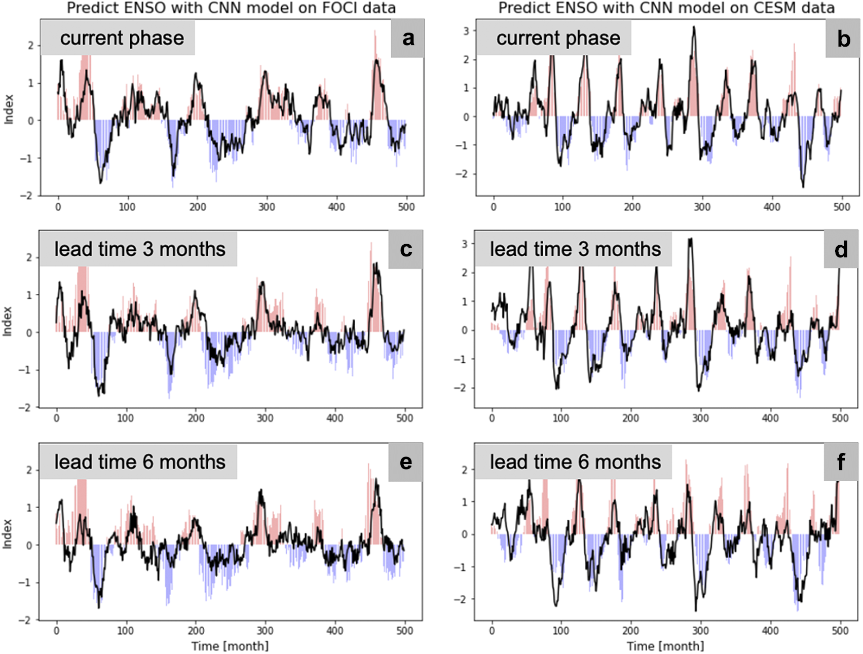
Figure 4. Fidelity check on the first 500 months of validation data: Compare predictions (black line) from CNN models on FOCI (left-hand side) and CESM data (right-hand side), respectively, compared to true targets shown as bar plot for various lead times. (a,b) Current phase. (c,d) Three months into the future. (e,f) Six months into the future.
Table 3. Evaluating model performance for predicting ENSO with CNN and LSTM models trained on FOCI and CESM data, respectively.

Note. The MSE and correlation (Correl) of predicted values and true targets are shown separately for training and validation data. ENSO phases at 3 and 6 months into the future are denoted as lead 3 and lead 6, respectively.
Abbreviations: CESM, community earth system model; FOCI, flexible ocean and climate infrastructure.
5. Discussion and Conclusion
In this work, we introduce a consistent and comprehensive collection of climate indices as a new benchmark data set. The collection is consistent in a sense that we use the output of ESM control runs to derive all indices. For FOCI and CESM control runs, we have 1000 and 999 years of monthly data, respectively, as an advantage compared to real-world data, since ML models require sufficient training data. The collection is comprehensive as we include a broad selection of known patterns, oscillations, and variability of the Earth system. The index collection is not complete since we focus on processes within the atmosphere, in the upper ocean and at the interface of ocean and atmosphere. However, our CICMoD data set serves as basis. Additionally, we provide an open-source framework that can to be extended and customized to individual needs including the application to further ESMs. This opens the door for collaboration in many ways. Our new data set allows researchers from the data science community to adapt existing ML models and develop new ML methods to tackle problems from the domain of climate science and get a deeper understanding of the Earth system. This requires involving scientists and practitioners from the domain of climate science.
To give an impression of how the new data set can be used, we apply several ML models on our CICMoD data set to predict Sahel rainfall and ENSO, respectively. In particular, we compare linear regression and MLP models to predict SPI. Results are shown in Section 4.1. Linear regression models perform slightly better on training data in terms of lower MSE combined with higher correlation of predictions and true targets, while MLP models show better performance on validation data, hence generalize better to unseen data. Comparing FOCI and CESM, we find lower MSE and higher correlation for linear regression and MLP models trained on indices derived from CESM data. As future work, these differences need to be further investigated.
As the second example, we predict current ENSO phase and ENSO phase 3 and 6 months into the future with CNN and LSTM models, respectively. Targets are derived from Niño 3.4 index and as predictors we use all remaining indices, excluding Niño indices. Input features and targets are found to be mostly uncorrelated with correlation coefficients in the range of −0.5 and 0.4. Results are shown in Section 4.2. We find a higher frequency of ENSO events in time series derived from CESM data, compared to FOCI. Still, periodicity for El Niño events falls in the expected range of 2–7 years for both ESMs. Overall, our CNN models slightly outperform LSTM models for predicting ENSO. Again, we look at MSE and correlation for evaluating model performance. The longer the target horizon, the worse the model performance in terms of higher MSE and lower correlation, as expected, since ENSO is a complex phenomenon that hinders long-term prediction beyond several months. As for Sahel rainfall prediction, our ML models perform better on indices derived from CESM data, compared to FOCI, which needs to be further investigated in future work.
ESMs aim to simulate Earth system dynamics. Different ESMs have their individual strengths and weaknesses. For our CICMoD data set, we use two distinct ESMs to derive all indices. Whenever we find some relation in one model context, we may try to reproduce our findings on the other model’s data to gain trust before repeating our experiments on real-world data. Like this, our CICMoD data set can help to reveal blind spots in ESMs and to find new causally linked modes within the real-world climate system. As future project, we plan to combine CICMoD with an extensive toolbox of explainable artificial intelligence (xAI) methods. Our new data set in combination with this xAI toolbox can then be used, for example, for data science competitions to tackle climate change and push the understanding of the climate system.
Author contribution
Conceptualization: M.L-H., W.R., M.C., P.K.; Data curation: M.L-H., S.W.; Data visualization: M.L-H., N.N.; Methodology: M.L-H., W.R., N.N.; Writing—original draft: M.L-H., W.R., S.W.; Writing—review and editing: M.C., P.K. All authors approved the final submitted draft.
Competing interest
The authors declare no competing interests exist.
Data availability statement
The software project for our CICMoD data set is hosted on GitHub: https://github.com/MarcoLandtHayen/climate_index_collection. This work is based on release number v2023.03.29.1, which is published on Zenodo, including the complete CICMoD data set as csv-file: https://doi.org/10.5281/zenodo.7779883. Furthermore, we reference a Docker container providing a Python environment with Jupyter notebooks, Tensorflow and climate_index_collection as pre-installed python package. Exemplary applications of our CICMoD data set to predict ENSO and Sahel rainfall are stored in a separate GitHub repository: https://github.com/MarcoLandtHayen/cicmod_application. Raw ESM data are stored on Zenodo: https://doi.org/10.5281/zenodo.7774316.
Ethics statement
The research meets all ethical guidelines, including adherence to the legal requirements of the study country.
Funding statement
This work was supported by the Helmholtz School for Marine Data Science (MarDATA) funded by the Helmholtz Association (Grant HIDSS-0005).


 Open access