


1. Introduction
The continental shelf of the East Siberian Sea (ESS) is the widest and shallowest in the World Ocean (Stein and others, Reference Stein, Macdonald, Stein and MacDonald2004; Semiletov and others, Reference Semiletov2005). The influence of the river runoff and oceanic inflow from both the Atlantic and the Pacific Ocean in combination with the shallow and extensive shelf make the East Siberian Sea one of the most active biogeochemical marine environments (Anderson and others, Reference Anderson2011).
Numerous studies indicate changes in the East Siberian Sea coastal environments: Overduin and others (Reference Overduin2014) show that coastal erosion along the East Siberian coast is strengthening. Along with a changing coastline, Shakhova and Semiletov (Reference Shakhova and Semiletov2007), Shakhova and others (Reference Shakhova2010a) and Semiletov and others (Reference Semiletov, Shakhova, Sergienko, Pipko and Dudarev2012) reported an increased degradation of submarine permafrost that is accompanied by an intensified release of methane through the shallow water column to the atmosphere. According to Shakhova and others (Reference Shakhova2010b), the methane trapped in the sediment there is climate-relevant because its release could contribute significantly to global warming.
Sea ice and particularly fast ice plays an important role for methane release and in coastal dynamics: According to Overduin and others (Reference Overduin2014), fast ice protects the coast from erosion by reducing the impact of waves. Moreover, it decouples ocean and atmosphere, and hence, prevents methane dissolved in the ocean to be released to the atmosphere prior to ice breakup (Shakhova and Semiletov, Reference Shakhova and Semiletov2007).
Although the East Siberian fast ice seems to play an important role for the regional gas and energy fluxes and the coastal environment as such, little is known about its seasonal evolution, the driving mechanisms and potential changes. According to Timokhov (Reference Timokhov1994), the East Siberian fast ice cover is considered to have similar characteristics as the Laptev Sea fast ice cover, due to the geographical similarity of the two regions. The study of Yu and others (Reference Yu, Stern, Fowler, Fetterer and Maslanik2013) that investigates arctic-wide changes in fast ice coverage indicates a decreasing winter extent of fast ice in the East Siberian Sea $\sim 10\%$ (23.6 × 10³ km2) per decade and a shortening of the fast ice season length (2.5 weeks per decade) between 1976 and 2007.
The aim of this study is to examine the seasonal and interannual variability of fast ice extent in the East Siberian Sea. Our first objective is to describe the seasonal fast ice cycle and evaluate changes occurring in the annual cycle during the past two decades. Understanding the mechanisms controlling fast ice development is essential for an assessment of future changes in fast ice regimes and their possible impact on the coastal environment. Since the Arctic fast ice seasonal cycle is strongly controlled by atmospheric processes (Divine and others, Reference Divine, Korsnes and Makshtas2004, Reference Divine, Korsnes, Makshtas, Godtliebsen and Svendsen2005; Mahoney and others, Reference Mahoney, Eicken, Gaylord and Shapiro2007, Reference Mahoney, Eicken, Gaylord and Gens2014; Selyuzhenok and others, Reference Selyuzhenok, Krumpen, Mahoney, Janout and Gerdes2015), our second objective is to link the observed variability of the fast ice seasonal cycle and extent to air temperature, wind direction, large-scale atmospheric circulation regime and sea ice drift.
2. Data and methods
2.1 Fast ice information
The information on fast ice extent from 1999 to 2021 was extracted from operational sea-ice charts provided by the Arctic and Antarctic Research Institute (AARI), Russia. Sea-ice conditions are mapped manually based on satellite imagery, ship reports, observations from polar meteorological stations, drift buoys and air reconnaissance flights. A detailed description of data sources and chart production is provided in Mahoney and others (Reference Mahoney, Barry, Smolyanitsky and Fetterer2008). The regional charts for the Eurasian Arctic shelf seas are available on a weekly basis in a vector Sea Ice Grid format (SIGRID-3). Fast ice is classified based on the criteria of immobility as well as other visual attributes such as absence of leads in the sea-ice cover. The information analysed by an expert is compiled for a period of 2–3 d prior to the issue date while the previous chart is used as a reference. Therefore, fast ice is defined as sea-ice cover which remains stationary along the coast during a period of 2–7 d. Overall, we analysed 858 maps for the period between January 1999 and September 2021. The fast ice extent was extracted for the region shown in Figure 1. Every annual cycle was described by two main key events (see definitions in Table 1 : key event 1 – beginning of fast ice season and key event 2 – end of fast ice season (dates when fast ice extent reaches/drops below an areal threshold)). Two additional key events (key event 3 and key event 4) were identified for the seasons when fast ice cover developed to a large extent or L-mode (the fast ice modes are described in Section Seasonal cycle and trends). This development is characterised by a rapid increase of fast ice extent from ~100 × 103 km2 to more than 250 × 103 km2 (Fig. 2b) over 2–4 weeks. Key events 3 and 4 indicate the beginning and the end of the period of rapid increase of fast ice extent. The arbitrary areal thresholds used to identify the key events of the fast ice annual cycle are given in Table 1. Due to gaps in the AARI dataset in 2002, 2003 and 2012, it was not possible to detect all key events describing the seasonal cycle and attribute season 2002 and 2003 to one of the fast ice modes. In order to fill the gaps and classify fast ice extent to L-/S-mode, we visually analysed MODIS thermal infrared imagery. In 2002, the L-mode configuration of the fast ice edge was observed for a short period, from mid-March to mid-April, followed by a breakout event. In 2003, all the small mode fast ice edge was observed from the beginning of March till the end of May.
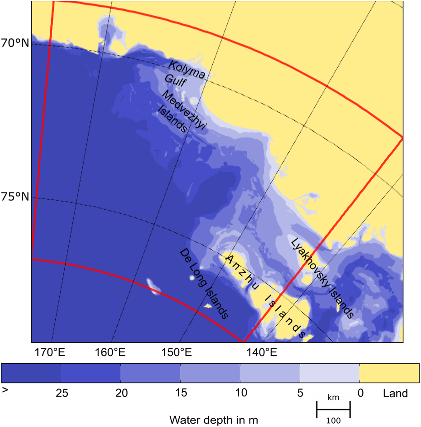
Figure 1. East Siberian Sea bathymetry from the International Bathymetric Chart of the Arctic Ocean (IBCAO Version 3, Jakobsson and others (Reference Jakobsson2012)). The shades of blue show the water depth (m). The red frame outlines the region for which fast ice extent and air temperature were extracted.

Figure 2. East Siberia Sea fast ice annual cycle for S-mode (a) and L-mode (b). The year corresponds to the year of winter when fast ice was fully developed (e.g. 1999 curve shows development of fast ice from October 1998 to August 1999).
Table 1. Key events and identification criteria

2.2 Atmospheric data
To investigate the influence of air temperature and wind direction on fast ice development, we used 3-hourly ERA5 Reanalysis 2-m air temperature and 10 m wind data. The mean daily air temperature was calculated over the marine part of the region shown in Figure 1. To analyse the frequencies of wind speed and directions, the daily values were extracted for the location centred in the area of the high interannual variation in fast ice extent (73.5° N/154.5° E).
To investigate the role of thermodynamic factors in annual fast evolution, we link the timing of fast ice key events to the onset of freezing and melting season, and freezing (FDDs) and thawing (TDDs) degree days. The dates of freezeup/melt onset were set as the first day of the week with continuous negative/positive regional mean air temperature. FDDs were calculated as the sum of negative air temperatures since the onset of freezeup. TDDs were calculated similarly, as the sum of positive air temperature since the onset of melt.
The influence of large-scale atmospheric circulation regime on the seasonal evolution of fast ice was investigated by comparing modes of the winter ice extent extracted from the satellite data to the polarity AO index. The AO index describes atmospheric mass exchange between the mid-latitudes and the Arctic (Thompson and Wallace, Reference Thompson and Wallace1998). The polarity of the AO index reflects a pattern of atmospheric circulation and sea-ice drift. During a positive AO phase in winter, the Beaufort Gyre is weak and the sea-ice transport away from the Siberian coast is increased. During the negative winter AO phase, the Beaufort Gyre is stronger and the sea-ice transport from the western to the eastern Arctic is increased resulting in sea-ice ridging and thickening at the Siberian coast (Rigor and others, Reference Rigor, Wallace and Colony2002).
2.3 Sea-ice drift and deformation
To further elaborate on the role of sea-ice deformation on the formation of fast ice extent in the East Siberian Sea, we derived the sea-ice convergence/divergence from sea-ice motion data. Comparing global sea-ice drift products with the buoy data, Gui and others (Reference Gui2020) showed that National Snow and Ice Data Center (NSIDC) and the Ocean and Sea Ice Satellite Application Facility (OSI-SAF) sea-ice drift products can be used for estimation of sea-ice deformation rates. However, NSIDC strongly underperformed relative to OSISAF when uncertainty was evaluated based on Synthetic Aperture Radar (SAR) data (Sumata and others, Reference Sumata, Kwok, Gerdes, Kauker and Karcher2015). The NSIDC datasets show persistent features due to a systematic error arising from the way satellite and buoy data are merged. These artefacts significantly impact calculation of sea-ice motion gradients, including divergence, convergence and shear. The OSISAF data do not show presence of such artificial structures (Szanyi and others, Reference Szanyi, Lukovich, Barber and Haller2016). In this study, we use recently released daily Global Low Resolution Sea Ice Drift data record (Release 1) that is based on the OSISAF sea-ice drift product (Lavergne and others, Reference Lavergne, Eastwood, Teffah, Schyberg and Breivik2010) to derive divergence in the region. The spatial resolution of the data is 75 km and they cover the period from 1998 to 2020. The order of the calculation is the following: ice divergence rate is calculated from daily ice motion, then the mean over an appropriate period is obtained. The divergence rate is obtained from daily ice speed components as follows:

Positive divergence values correspond to ice opening, e.g. lead formation, while negative values indicate pressure in pack ice that might result in sea-ice ridging/rafting or closing of leads.
3. Results and discussion
3.1 Seasonal cycle and trends
The fast ice season in the East Siberian Sea lasts from November until August. The maximal winter extent is reached in February–May and shows high interannual variability (Fig. 2). The winter extent is characterised by a bimodal distribution (Fig. 3): There are two distinctive modes at 170 − 190 × 103 km2 and 270 − 290 × 103 km2 separated by a significant drop in frequencies at 250 × 103 km2. We classified fast ice seasons to small (S-mode) and large (L-mode) extent seasons applying 250 × 103 km2 threshold on the mean February–May fast ice extent. Due to the gaps in the ARRI dataset, the seasons 2002 and 2003 were classified based on the visual inspection of MODIS thermal infrared imagery using EOSDIS Worldview service.

Figure 3. Frequency of fast ice mean February–May extent. The distribution of winter fast ice extent has two clear modes at 170 − 190 × 103 km2 and 270 − 290 × 103 km2, which correspond to S- and L-mode of fast ice configuration.
The L- and S-modes occurred with almost the same frequency throughout the 23-years investigation period. The L-mode developed during ten seasons. In winter 1999, 2001, 2005–2006, 2010, 2013–2014, 2016, 2018 and 2021, fast ice was in its large configuration until the summer breakup. During the winter 2002, 2004, 2012 and 2015, the large extent developed only for a short period of 1–2 weeks and then reduced to the small extent which persisted until the summer breakup. We refer to these seasons as not-classified. The S-mode was observed during nine seasons in winter: 2000, 2003, 2007–2009, 2011, 2017, 2019 and 2020.
During small extent mode (S-mode), the fast ice develops gradually in fall, reaches its maximal winter extent in March–April and gradually disintegrates in June–August (Fig. 2). The S-mode fast ice develops an arch-shaped edge going from the Anzhu Islands to the mainland (Fig. 4). The large mode (L-mode) is characterised by a gradual development in fall, followed by a rapid fast ice areal growth in February–May (Fig. 2).

Figure 4. Mean February–May frequency of fast ice occurrence for (a) L- and (b) S-mode.
The breakup of L-mode fast ice takes place in June–August. As for the S-mode, it fully disintegrates during these 3 months. Figure 4 shows the frequency of fast ice occurrence characteristic for L- and S-modes. Compared to the S-mode, the fast ice extends further north and its edge forms a straight NW-SE line going from the eastern Anzhu Island to the mainland on the east of the sea.
The timing of the onset and trends of key events are presented in Tables 2 and 3, respectively. We found that the variability of the onset of the beginning and end of the fast ice season is low (±10 d). Contrary, the timing of L-mode development and its fully developed L-mode are highly variable (~±30 d).
Table 2. Variability of dates of the key events 1999–2021

Table 3. Trends in timing of key events and periods of annual fast ice cycle 1999–2021

There is a tendency towards earlier end of fast ice season (statistically significant at 99 $\%$ confidence level; Table 3). The tendency towards a later beginning of the fast ice season has a low confidence level. Nevertheless, the overall length of the fast ice season decreases by 1.5 d per year (2 weeks per decade) during 1999–2021. A slightly higher tendency of 2.5 weeks per decade for the East Siberian fast ice was found between 1976 and 2007 (Yu and others, Reference Yu, Stern, Fowler, Fetterer and Maslanik2013).
Figure 5 shows a time series of mean winter fast ice area between 1999 and 2021. These show decreasing trends of fast ice area for the entire time series from 1999 to 2021, as well as individually for S- (the lowest trend line in Fig. 3) and L- (the upper trend line in Fig. 5) fast ice modes. However, the trends have low statistical significance (p-value >0.05) due to large interannual variability.

Figure 5. Mean winter fast ice extent. The blue line shows mean February–May fast ice extent between 1999 and 2021. The black dash lines correspond to the linear trend calculated for the entire time series (total) and for the seasons of L- and S-mode fast ice configuration. The seasons attributed by short events of L-mode fast ice configuration are not marked by circle. Due to a gap in the AARI sea-ice maps, the data for winter 2002 and 2003 are missing.
3.2 Role of the atmosphere and sea-ice drift
The correlation coefficient between the timing of the key events and the air-temperature derived onset of freezeup and melt is presented in Table 4. We found statistically significant relations between the onset of freezeup and the beginning of the fast ice season. The variability of FDDs and TDDs accumulated prior to the key events (Table 5) is higher for the beginning and end of fast ice season ($\sim 50\%$ ) and lower for the events of L-mode development (<20%). The high correlation between onset of freezeup and beginning of fast ice season confirms the importance of thermodynamic processes for the fast ice annual cycle (Table 4). Overall, low variability of FDDs and TDDs accumulated prior to the onset of all key events (Table 5) suggests that air temperature plays an important role in seasonal fast ice cycle.
Table 4. Correlation (R) between key events, freezeup and melt onset

Table 5. FDDs and TDDs accumulated prior to the key events 1999–2019

To assess the potential influence of the large-scale atmospheric circulation on the evolution of the fast ice extent in winter, we compare the AO index with winter fast ice extent. Figure 6 shows the time series of cumulative January–March AO indices for 1999–2021 aligned with the occurrence of L-/S-modes of fast ice extent. Overall we find that the fast ice L-mode coincides well with the phases of negative AO index in January–March. Moreover, all of the seasons with S-mode show a positive AO index. The high correlation coefficient of 0.9 between the polarity of AO and the presence of fast ice L-/S-mode indicates that there is a strong linkage between bi-modal fast ice distribution and patterns of atmospheric circulation. The difference between the L-/S-mode local atmospheric winds patter can be clearly seen from average February–May wind speed and direction (Fig. 7). The L-mode seasons are characterised by stronger wind speeds blowing from the northeast towards the East Siberian Sea coast. In contrast the offshore wind predominates during S-mode seasons.

Figure 6. Time series of monthly AO index and cumulative January–March AO index. The vertical bars mark February–May period when fast ice extent reaches its maxima. The colour of the bars correspond to the fast ice mode formed during the season.

Figure 7. Average February–May wind speed and direction rose for (a) L- and (b) S-mode seasons. The red frame outlines the region of interest (Fig. 1).
Figure 8 shows the February–May distribution of wind direction and speed for the seasons characterised by L- and S- fast ice modes. The L-mode histogram (Fig. 8a) shows a unimodal distribution of wind direction with a pronounced mode for winds from N-NNE direction. The modal direction also shows the highest occurrence of strong winds (10 − 15 m ⋅ s−1). Compared to L-mode, the S-mode histogram (Fig. 8b) shows a more uniform distribution of wind frequencies with slightly higher values for winds from N-NNW and S-SSW directions.

Figure 8. Average February–May wind rose histograms for (a) L- and (b) S-mode seasons. The bars direction corresponds to the direction the wind blows from.
A good agreement between the seasons with L-/S-modes and negative/positive winter AO index suggests that there is a linkage between the general pattern of Arctic atmospheric circulation and the fast ice extent. Rigor and others (Reference Rigor, Wallace and Colony2002) showed that during negative AO phases, the sea ice is imported to the East Siberian Sea from the east. A positive AO phase is characterised by presence of a weak cyclonic gyre on the east of the region which prevents sea-ice inflow to the western part of East Siberian sea. During negative AO phases, the sea-ice import to the East Siberian Sea might result in higher rates of sea-ice ridging in the region compared to seasons where sea ice in the East Siberian sea was formed locally and is likely less thick or deformed. Therefore, during negative AO phases, formation of sea-ice ridges that are thick enough to ground and thereby stabilise the extensive fast ice cover is more likely. The derived sea-ice divergence rates confirm that the L-mode fast ice seasons are characterised by higher convergence rate (Fig. 9a), compared to lower convergence rate during the S-mode fast ice season (Fig. 9b). During L-mode seasons, convergence dominates in the region, indicating lead closing or ridging. On the other hand, during S-mode seasons, zones divergence associated with ice-opening are observed seaward the fast ice edge.

Figure 9. Mean February–May sea-ice divergence rate (left) L- and (right) S-mode occurred during 1999–2021. Negative values depict sea-ice convergence. The areas with no data are depicted with black dots. The position of fast ice edge is drawn as the black line.
Mahoney and others (Reference Mahoney, Eicken, Gaylord and Gens2014) suggested that the location of grounded ice ridges can be inferred from the convergence of fast ice edges (‘nodes’) on frequency occurrence maps. Figure 4a shows that such ‘nodes’ occur north-east of Anzhu Islands and north of small shoals in the central part of the region. The shape of the fast ice edge during the L-mode also coincides with the locations of large stamukhi observed in 1987–2002 (Gorbunov and others, Reference Gorbunov, Losev and Dyment2007). Therefore, we suggest that the development of large fast ice extent in the East Siberian Sea is controlled by the formation of grounded sea-ice features, i.e. stamukhi and ridges which in turn are governed by a pattern of atmospheric circulation characterised by low AO.
4. Conclusions
By using AARI operational sea-ice charts, we analysed seasonal and interannual variability of fast ice extent in the East Siberian Sea between 1999 and 2021. We identified key events in each annual fast ice cycle and linked the occurrence of these events to air-temperature derived freezeup and melt onset, and FDDs and TDDs. The analysis reveals that the beginning and the end of the fast ice season is controlled by thermodynamic factors, i.e. onset of freezing temperatures and accumulated TDDs. On the multiyear time scale, we found a tendency towards a shorter fast ice season. The duration of the fast ice season reduces by 2 weeks per decade, which is in agreement with the Arctic-wide trend of other fast ice regions (Yu and others, Reference Yu, Stern, Fowler, Fetterer and Maslanik2013), however, the trends are not statistically significant. The spatial configuration of winter fast ice extent in the East Siberian Sea is characterised by small (S-mode) and large (L-mode) modes with significantly different extent. The two modes developed with equal frequency between 1999 and 2021. The L-mode is associated with an increased north-northeasterly wind frequency in winter. The S-mode is characterised by lower northerly and higher southwesterly wind frequency with overall domination of offshore wind direction. A comparison of winter AO index with the occurrence of S- and L-modes suggests that the pattern of atmospheric circulation controls the development of either mode. During negative winter AO, enhanced sea-ice deformation at the Siberian coast leads to formation of grounded sea-ice features on the shoals of the East Siberian Sea. These grounded features promote increased fast ice extension to L-mode. A positive AO circulation pattern leads to sea-ice export from the Siberian coast resulting in lower deformation rates. Then, less deformed grounded sea ice does not allow fast ice stabilisation farther offshore leading to the persistence of the S-mode during the season.
Acknowledgements
We thank Matti Leppäranta for his valuable comments. This work was carried out as part of the Russian–German research cooperation QUARCCS funded by the BMBF under grant 03F0777A and CATS under grant 63A0028 and funded by RFBR, project number 19-35-60033.


 Open access