Design and applications of drilling trajectory measurement instrumentation in an ultra-deep borehole based on a fiber-optic gyro

Liu, Yimin; Wang, Chenghu; Luo, Guangqiang; Ji, Weifeng

doi:https://doi.org/10.5194/gi-9-79-2020

Articles | Volume 9, issue 1

https://doi.org/10.5194/gi-9-79-2020

Articles | Volume 9, issue 1

Research article

19 Mar 2020

Research article |

| 19 Mar 2020

Design and applications of drilling trajectory measurement instrumentation in an ultra-deep borehole based on a fiber-optic gyro

Yimin Liu, Chenghu Wang, Guangqiang Luo, and Weifeng Ji

Abstract

The working environment in hot dry rock boreholes, encountered in deep geothermal investigation drilling and ultra-deep geological drilling (up to 5000 m), is very difficult at the present stage. We have developed a drilling trajectory measuring instrumentation (DTMI), which is based on the interference fiber-optic gyro (FOG). This can work continuously, for 4 h, in an environment where the ambient temperature does not exceed 270 ^∘C and the pressure does not exceed 120 MPa. The DTMI is mainly divided into three parts: an external confining tube, a metal vacuum flask, and a FOG measurement probe. Here, we focus on the mechanical design, strength, and pressure field simulation analysis for the external tube, the structural design and temperature field simulation analysis for the vacuum flask, and the FOG Shupe error analysis and compensation in the temperature field. Finally, through the engineering applications of the SK-2 east borehole of the China Continental Scientific Drilling (CCSD) project and the geothermal well of Xingreguan-2, the data measurements of the drilling trajectory were used to analyze the stability of the DTMI. The instrument realizes long-duration, high-stability work in the process of making trajectory measurements in an ultra-deep hole. The instrument has the characteristic of anti-electromagnetic interference and enables work to be carried out in the blind zone of existing technologies and instrumentation. Therefore, DTMI has great potential in the promotion and development of geological drilling technology.

Download & links

Article (PDF, 4556 KB)

How to cite

How to cite.

Dates

Received: 04 Nov 2019 – Discussion started: 21 Nov 2019 – Revised: 05 Feb 2020 – Accepted: 13 Feb 2020 – Published: 19 Mar 2020

1 Introduction

With the recent rapid development of the national economy, shortages in resources and energy have become major barriers to economic development. In order to obtain more resources and energy, we now need to explore deeper into the Earth's crust. Therefore, the depth of drill holes for mineral resource exploration and extraction is constantly increasing. Furthermore, geothermal energy and shale gas are considered to be new “green energies” that can maintain sustainable development, which is of both domestic and foreign concern. Therefore, the development of drilling engineering, in the field of high-temperature geothermal energy and shale gas, is included in the development plan of China (Chen et al., 2015). With increases in borehole depths, there is also an increase in temperature. In general, the temperature gradient for a normal formation is about $3^{\circ} C / 100 m$ ; the maximum temperature of a 3000 m deep oil and gas well can reach over 100 ^∘C. When the borehole depth reaches around 8000 m, the temperature will reach 250 ^∘C. In hot dry rock, areas of high geothermal energy, and other areas with anomalous geothermal gradients, the temperature will be higher (Osipova et al., 2015; Chen et al., 2015). When the depth of the borehole (well) increases, the degree of borehole deviation also increases. Borehole deviation will have a significant impact on the quality of the borehole and construction safety. With the increasing depth of deep mineral resource exploration and geothermal resource exploration and development, the drilling path or trajectory needs to be more and more accurate (Xu et al., 1996). Therefore, borehole deviation and drilling trajectory must be measured to provide technical support for drilling construction.

One of the main technical problems in ultra-deep borehole drilling construction is how to measure the drilling trajectory in a high-temperature environment while ensuring measurement accuracy. At present, the drilling trajectory measurement technique is to measure the zenith angle of the hole's (well's) body axis (the angle between the tangent of the wellbore axis and the vertical), the azimuth angle (the direction of the horizontal projection of the tangential line of the wellbore axis), and the depth of the hole (the depth position of the measuring point in the well). These three main geometric parameters are then used in an appropriate calculation method to calculate the spatial position of the measured point indirectly, so as to obtain the trajectory data for the hole (well) (Xiao et al., 1989). Figure 1 shows the coordinate system of a borehole trajectory.

https://www.geosci-instrum-method-data-syst.net/9/79/2020/gi-9-79-2020-f01

Figure 1Coordinate system of a borehole trajectory.

Download

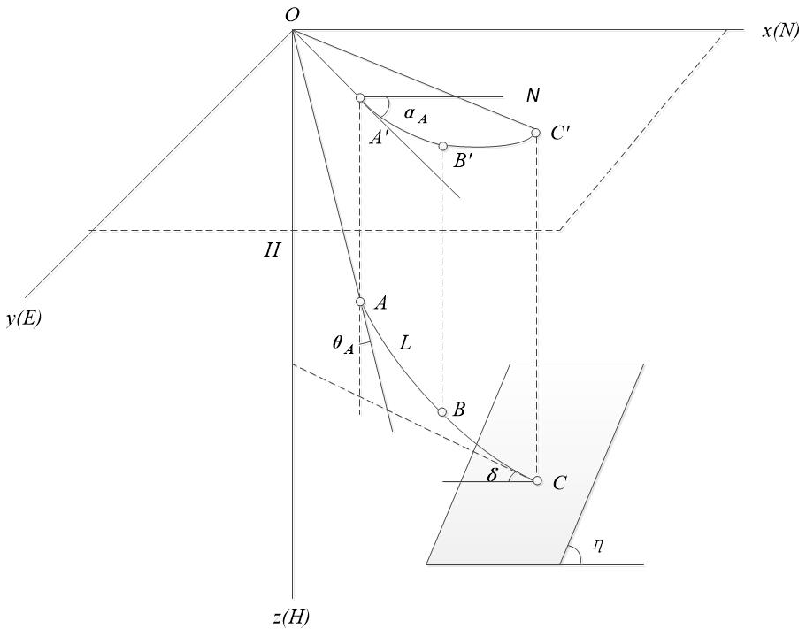
As shown in Fig. 1, the curve OAC is the trajectory of the borehole in the coordinate system, the zenith angle (θ_A) is the angle between the tangent at the point and the vertical line, the azimuth angle (α_A) is the angle between the projection of the tangent line onto the horizontal plane and the true north direction, and the hole depth (H_A) is the distance from the orifice O to the bore axis of the point.

The hole depth can be measured by the length of the drill pipe or cable under the hole. The measurement of zenith angle generally uses a sensor based on the measurement principle of liquid level, suspension principle and gravitational acceleration, and the precision is relatively high. The azimuth measurement is usually of the following two types: one uses the principle of the Earth's magnetic field, and the other uses the principle of inertial navigation. The borehole inclinometer, which is based on the principle of geomagnetic field orientation, is only suitable for non-magnetic interference or weak magnetic mining areas (Sedlak, 1994). In strongly magnetic mining areas or in magnetic interference drilling, due to the interference of the Earth's magnetic field or metal shielding (magnetic mining area, instrument casing, and drill pipe casing), the accuracy of this type of instrument does not meet the measurement requirements (Yamaguchi et al., 2015). In order to solve the problem of borehole inclination in the case of strong magnetic interference (inside the drill pipe, inside the casing, etc.), the azimuth is generally measured by optical fiber or dynamic tuning gyroscope, based on the principle of inertial navigation. Some existing fiber-optic gyro (FOG)-based drilling trajectory measuring instrumentation (DTMI) are shown in Table 1 (Mass et al., 2007).

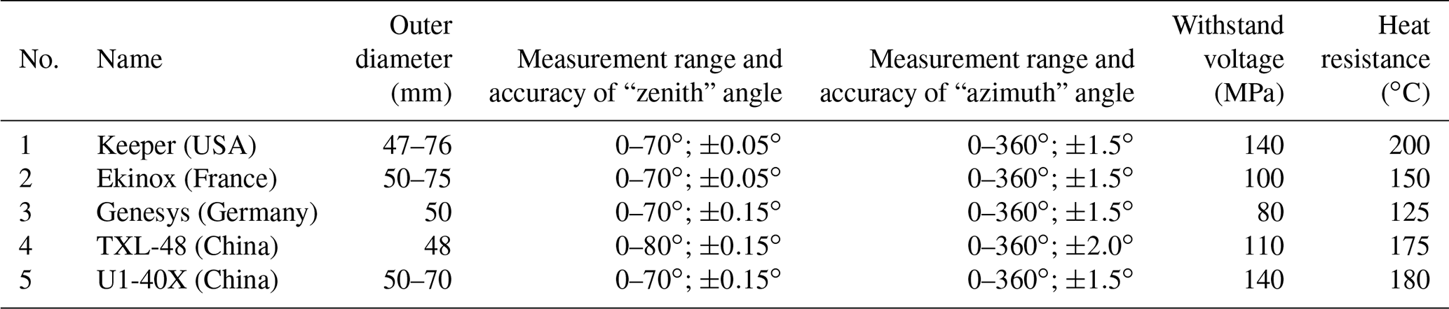
Table 1Technical parameters of some DTMIs based on FOG.

Download Print Version | Download XLSX

From Table 1, we can know that the instrument that can withstand the highest temperature and pressure is the Keeper type produced in the US, and the maximum temperature is 200 ^∘C; the maximum pressure is 140 MPa. However, as mentioned in the first paragraph, the temperature can reach 250 ^∘C or even higher in a hot dry rock borehole or an ultra-deep borehole. Therefore, there is a lack of drilling trajectory measurement instruments and corresponding technologies for such high-temperature and high-pressure environments. There are also many problems in the practical application of the drilling trajectory measurement. Therefore, research on drilling measurement technology for high-temperature and high-pressure environments, encountered in ultra-deep drilling, is of great significance. This technology can be used for new energy, ultra-deep oil and gas development, high-temperature geothermal energy, hot dry rock development drilling engineering, scientific drilling engineering, ultra-deep mineral resource drilling engineering, and oil and gas drilling engineering.

Here, we look at working environments with a maximum temperature not exceeding 270 ^∘C and pressures not exceeding 120 MPa. A thermal simulation analysis of a metal vacuum flask and pressure simulation modeling of the external confining tube are presented. A design scheme for DTMI is proposed and optimized. Through the field engineering application in the China Continental Scientific Drilling (CCSD) project and in geothermal development drilling, a long-duration, high-performance DTMI for deep hole trajectory measurement has been realized. This is of great significance for promoting the development of geological drilling.

2 Design and principles of DTMI

2.1 Configuration of DTMI

DTMI is an important instrument for investigating drilling construction quality and trajectory parameters in anti-magnetic interference drilling engineering. The DTMI is mainly composed of an external confining tube, a metal vacuum flask, and an FOG measuring probe, shown in Fig. 2.

https://www.geosci-instrum-method-data-syst.net/9/79/2020/gi-9-79-2020-f02

Figure 2Photos of external confining tube, metal vacuum flask, and FOG measurement probe.

Download

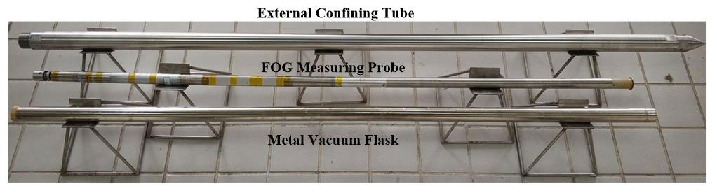
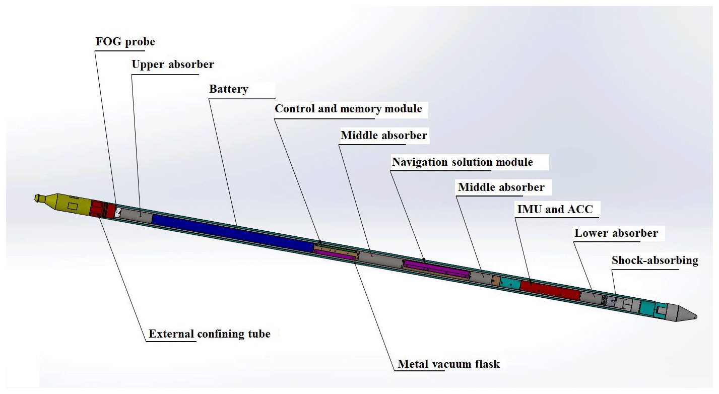
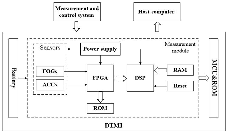
The external confining tube is the outermost layer, a threaded interface is equipped with a high-pressure metal sealing ring to ensure that the maximum pressure reached is 120 MPa. For downhole measurements, it is equipped with a shock-proof guide joint and a centralizer. The metal vacuum flask forms the middle layer, which is equipped with four heat absorbers and shock absorbers in the upper, middle, and lower parts. These ensure that, as the temperature rises externally to 270 ^∘C, during the 4 h of operation the internal temperature of the bottle does not exceed 90 ^∘C. The FOG measurement storage probe forms the innermost level, mainly comprised of an inertial measurement unit (IMU) sensor components, storage control module, navigation solver module, and a high-temperature battery. Its function is to realize multi-point azimuth and inclination measurements and storage (Liu, 2016; Lin et al., 2015). The internal structural diagram of the DTMI is shown in Fig. 3.

https://www.geosci-instrum-method-data-syst.net/9/79/2020/gi-9-79-2020-f03

Figure 3Internal structural diagram of DTMI.

Download

The measurement flowchart of the DTMI is shown in Fig. 4. The DTMI is lowered and lifted by a wire rope connection, and the data measured, during operation, are stored in the probe's memory, in real time. When the measurements are completed, the trajectory measuring probe is taken out of the borehole, the storage module in the FOG probe is connected to the ground laptop, through the data line, and the data stored in the probe are read by the upper computer measurement software. Data processing and display are performed, thereby giving the results of the trajectory measurements.

https://www.geosci-instrum-method-data-syst.net/9/79/2020/gi-9-79-2020-f04

Figure 4Hardware diagram of DTMI.

Download

2.2 Design and principles of measurement module

2.2.1 Measurement module design

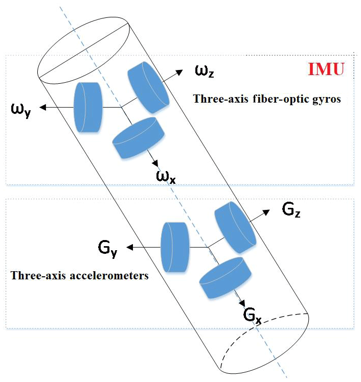
The measurement module consists of a three-axis fiber-optic gyroscope (inertial measurement unit) and a three-axis accelerometer (acceleration measuring unit), which are orthogonal to each other, as shown in Fig. 5.

https://www.geosci-instrum-method-data-syst.net/9/79/2020/gi-9-79-2020-f05

Figure 5Composition diagram of the three-axis measurement module.

Download

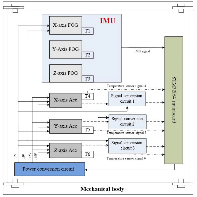
The measurement module uses a module design method; it consists of a three-axis accelerometer sensor module, a three-axis FOG sensor module (IMU), a temperature sensor module, a signal conditioning module, a high-precision A/D conversion module, a navigation calculation processing module, and a high-temperature power module, which are shown in Fig. 6.

https://www.geosci-instrum-method-data-syst.net/9/79/2020/gi-9-79-2020-f06

Figure 6Figure of measurement principles.

Download

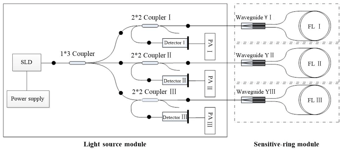
The key component is the FOG measurement component. This is composed of an interference fiber gyro (I-FOG), an optical path portion, and a circuit portion. According to the three-axis integrated design, three interferometric fiber-optic gyroscopes (I-FOG) are fixed, respectively, on the three coordinate axes of the carrier coordinate system, which are orthogonal each other. As shown in Fig. 7, each single-axis optical path is partially composed of a light source (divided by a super-luminescent diode (SLD) tube), a coupler, an integrated optical modulator (referred to as a waveguide-Y), and an optical fiber ring (a special process used for a polarization-maintaining optical fiber). The detector consists of five major components, and three FOGs share one SLD light source. Other functional modules adopt a mature all-digital closed environmental biasing scheme. This design has advantages of low cost, small size, and high stability. Meanwhile, the design of the inertial navigation measurement module focuses on the assembly process, low thermal power, overall electromagnetic compatibility, and anti-interference (Titterton and Weston, 2004; Savage and Paul, 2013).

https://www.geosci-instrum-method-data-syst.net/9/79/2020/gi-9-79-2020-f07

Figure 7Composition diagram of IMU.

Download

2.2.2 Measurement principles

Due to the narrow space inside the borehole, it is very difficult to install a stable physical measurement platform. Therefore, the instrument uses the strapdown inertial navigation technology to realize the function of navigation by using the fiber-optic gyroscope, accelerometer, and trajectory calculation model (Grewal et al., 2007). Among them, the three-axis accelerometer measures the acceleration in three directions, and the acceleration value can be used to obtain the displacement, in three directions, by double integration with respect to time; the three-axis fiber-optic gyroscopes measure the rotational speed of the carrier in three directions, and the corresponding rotation angle can be obtained by integrating with respect to time.

Using the three-axis displacement and rotation angle, the attitude matrix is solved by the space coordinate system variation, the drilling trajectory calculation model, the Euler angle coordinate transformation, and the quaternion method; when the rigid body is rotated around an axis, the angular position of the rotating rigid body can be calculated (Çelikel and Sametoğlu, 2012). The rotation of the carrier coordinate system, relative to the navigation coordinate system, is shown in Eq. (1).

\begin{matrix} (1) & \dot{Λ} = \frac{1}{2} W (w_{n b}^{b}) Λ \end{matrix}

There is Λ = [\begin{array}{c} q_{0} \\ q_{1} \\ q_{2} \\ q_{3} \end{array}],

W (w_{n b}^{b}) = [\begin{array}{cccc} 0 & - w_{n b x}^{b} & - w_{n b y}^{b} & - w_{n b z}^{b} \\ w_{n b z}^{b} & 0 & w_{n b z}^{b} & - w_{n b y}^{b} \\ w_{n b y}^{b} & w_{n b z}^{b} & 0 & w_{n b x}^{b} \\ w_{n b z}^{b} & w_{n b y}^{b} & - w_{n b x}^{b} & 0 \end{array}] .

The fourth-order Runge–Kutta (R–K) method is used to solve the ordinary differential equation (Bernardo and Shu, 1989); the azimuth α, the zenith θ, and the tool face angle β can be obtained by Eq. (2).

\begin{matrix} (2) & \{\begin{cases} \tan θ = \frac{\sqrt{G_{X}^{2} + G_{Y}^{2}}}{G_{Z}} \\ \sin θ = \frac{G_{Z}}{\sqrt{G_{X}^{2} + G_{Y}^{2} + G_{Z}^{2}}} \end{cases} \{\begin{cases} α = \arctan [\frac{2 (q_{1} q_{2} + q_{0} q_{3})}{q_{0}^{2} + q_{1}^{2} - q_{2}^{2} - q_{3}^{2}}] \\ θ = \arcsin [2 (q_{1} q_{3} - q_{0} q_{2})] \\ β = \arctan [\frac{2 (q_{2} q_{3} + q_{0} q_{1})}{q_{0}^{2} + q_{1}^{2} - q_{2}^{2} + q_{3}^{2}}] \end{cases} \end{matrix}

\begin{matrix} (3) & \{\begin{cases} q_{0} = \cos \frac{α}{2} \\ q_{1} = \sin \frac{α}{2} \cos β_{x} \\ q_{2} = \sin \frac{α}{2} \cos β_{y} \\ q_{3} = \sin \frac{α}{2} \cos β_{z} \end{cases}, \end{matrix}

where α is the angle of rotation about the axis of rotation, and G_X, G_Y, and G_Z are components of the acceleration in the x, y, and z directions, respectively; cos β_x, cos β_y, and cos β_z are components of the axis of rotation in the x, y, and z directions, respectively.

2.3 Technical parameters

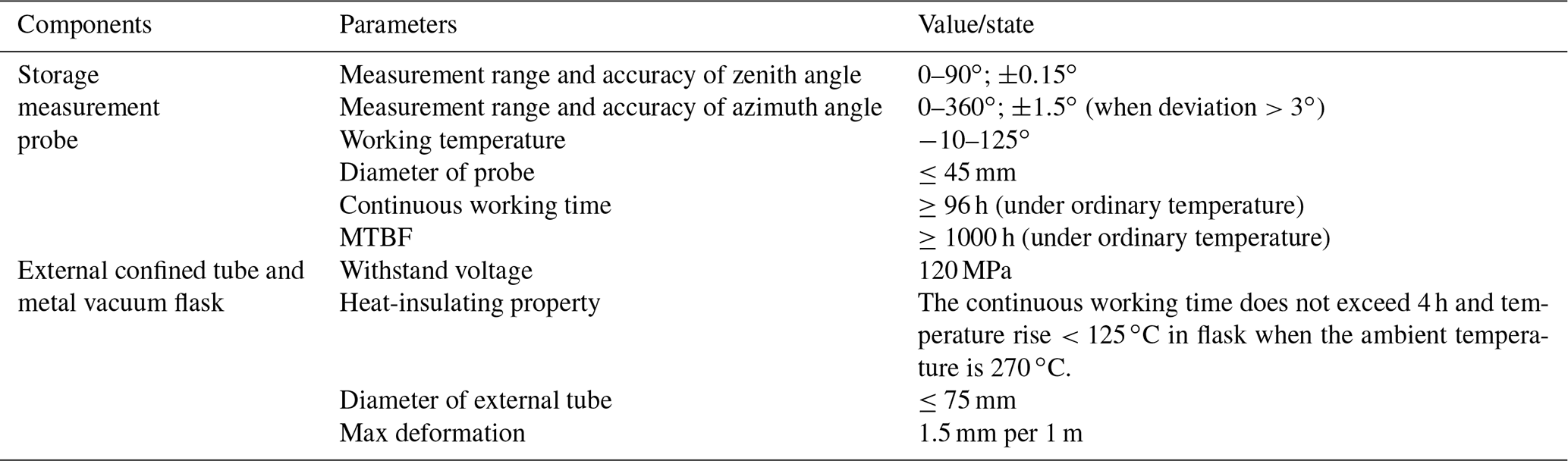
The technical parameters of the DTMI based on the FOG are shown in Table 2.

Table 2Key technical parameters of the DTMI. MTBF is the mean time between failure.

Download Print Version | Download XLSX

3 Key technologies of the DTMI

This section focuses on the temperature resistance and measurement accuracy of the DTMI. For this, we look at three aspects: mechanical design of the external confining tube, structural design of the vacuum flask, and FOG error compensation. This is to ensure that the DTMI can work for a long duration with high performance in the ultra-deep hole trajectory measurement process and meets the design parameters.

3.1 External confining tube

The main function of the external confining tube is to ensure that the DTMI can withstand an external pressure of up to 120 MPa, during 4 h of working time. Due to the complexity of the loads when the DTMI is doing actual drilling work, this section uses finite element analysis software to accurately model and analyze its mechanical state. Based on the analysis of the overall model to the local components, a mechanical simulation of the external confining tube is carried out. The stress–strain distribution and deformation of each detail position, under different loads, are compared and analyzed (Tavio and Tata, 2009).

Joints of drilling trajectory measuring instruments, at home and abroad, widely use tapered thread, trapezoidal buckles. One of the reasons for this is high strength; the second is that they are simpler than rectangular buckles. In addition, they are wear-resistant and easier to unscrew than circular threads (Kielbassa et al., 2009). Sealing and connection of the DTMI used tapered threads; the simplified schematic of a threaded-tooth-type, trapezoidal buckle is shown in Fig. 8a. The connection and sealing of the DTMI are achieved by the pre-tightening force on the thread end face and the shoulder surface of the threaded shoulder. The pre-load force, generated by the threaded buckle, has an important effect on the critical load of the confining probe joint, the fatigue damage resistance, the axial load resistance, and the sealing of the shoulder contact surface, as shown in Fig. 8b.

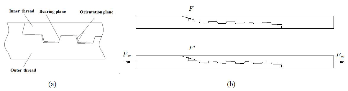
https://www.geosci-instrum-method-data-syst.net/9/79/2020/gi-9-79-2020-f08

Figure 8(a) Diagram of internal and external thread matching; (b) effect of axial load on pre-load.

Download

3.1.1 Establishment of finite element model for threaded connection

For the material of the external confining probe tube, 17-4PH precipitation-type hardened stainless steel was selected. This has good mechanical properties, good temperature resistance, and slow heat conduction. The sealing joint is made of 30CrMnSiA using heat treatment. The technical parameters of the two materials are shown in Table 3 (Wen et al., 2010).

Table 3Material parameters of the confined tube.

Download Print Version | Download XLSX

https://www.geosci-instrum-method-data-syst.net/9/79/2020/gi-9-79-2020-f09

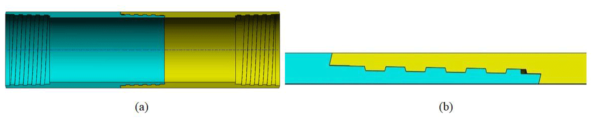
Figure 9(a) Connector thread assembly drawing; (b) model simplified diagram of two-dimensional axisymmetric.

Download

We used the Ansys workbench platform to build a simplified model of the thread, accurately assemble it, and finally import it into the Ansys platform, for accurate mechanical simulation analysis, as shown in Fig. 9.

3.1.2 Simulation of the pressure field and optimization of the structural parameters

This section focuses on optimizing the design parameters of the probe, from the internal and external diameter (wall thickness), thread taper, thread height, and pitch. From field experience, the outer diameter of the probe tube was designed to be 73 mm, and the inner diameter selected was 68 mm; 67.5, 67, 66.5, and 66 mm were used for finite element analysis.

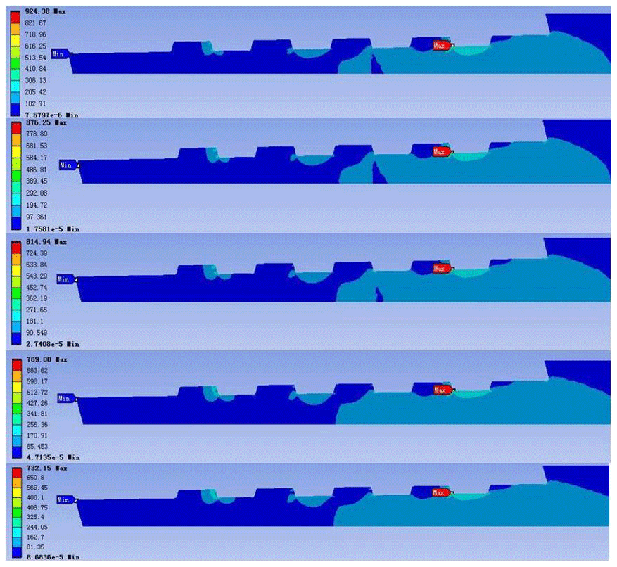
https://www.geosci-instrum-method-data-syst.net/9/79/2020/gi-9-79-2020-f10

Figure 10The stress nephogram of the external thread of the confined probe joint (the inner diameters from top to bottom are 68, 67.5, 67, 66.5, and 66 mm, respectively).

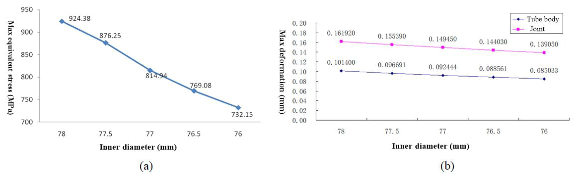
https://www.geosci-instrum-method-data-syst.net/9/79/2020/gi-9-79-2020-f11

Figure 11(a) The trend diagram of the maximum equivalent stress with inner diameter decreases; (b) the trend diagram of the maximum total deformation with inner diameter decreases.

Download

Effect of local thickening of confined probe joint on connection strength

Local thickening of the ends of the joint thread is one common processes for improving the strength of the confining probe joint (Vasudevan et al., 2013). According to the work experience and the actual situation, the outer diameter of the probe tube is designed to be 73 mm, and the inner diameter of the pipe body is selected as 68 mm; 67.5, 67, 66.5, and 66 mm were used for finite element analysis. The equivalent stress value of the thread, the von Mises stress, the maximum equivalent stress value, and the stress contour are compared and evaluated. The stress and deformation of the local details of the threaded joint are also evaluation indexes. The results are shown in Figs. 10 and 11.

From the finite element analysis results (Fig. 11), the following conclusion can be obtained: with a decrease in the inner diameter of the probe joint (i.e., the thickness component is thickened), the maximum equivalent stress at the joint thread is gradually reduced and joint strength is increased by 20.8 %. At the same time, the maximum total deformation of the confining probe and joint is gradually reduced, indicating that the stress distribution inside the thread is more balanced. Therefore, the inner diameter set at 67 mm greatly improves the connection strength of the confining probe.

Effect of thread taper on joint strength

The thread parameters of the confining tube are selected from the national standard equipment standard GB/T 16951–1997 (Neq ISO 10098: 1992, 1997). For the simulation analysis, five sets of taper were selected; these were 1:15, 1:20, 1:25, 1:30, and 1:36. The results of finite element calculation are shown in Figs. 12 and 13.

We comprehensively analyzed the maximum equivalent stress of the pipe body and the joint with different tapers. When the taper of the thread is around 1:25, the overall joint strength of the pressure probe tube is the greatest.

Effect of thread height on joint strength

Overall, seven thread heights (0.8, 0.9, 1.0, 1.1, 1.2, 1.3, and 1.5 mm) were selected for simulation analysis, and the results of the finite element calculation are shown in Figs. 14 and 15.

https://www.geosci-instrum-method-data-syst.net/9/79/2020/gi-9-79-2020-f12

Figure 12The stress nephogram of the external thread of the confining probe joint (the tapers from top to bottom are 1:15, 1:20, 1:25, 1:30, and 1:36).

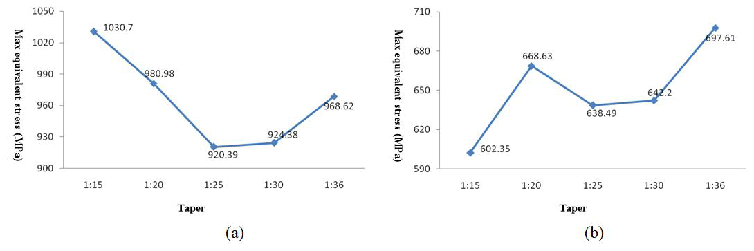
https://www.geosci-instrum-method-data-syst.net/9/79/2020/gi-9-79-2020-f13

Figure 13(a) Relationship between thread taper and the maximum equivalent stress of tube body; (b) relationship between thread taper and the maximum equivalent stress of joint.

Download

https://www.geosci-instrum-method-data-syst.net/9/79/2020/gi-9-79-2020-f14

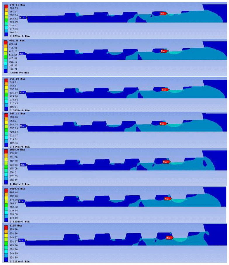
Figure 14The stress nephogram of the external thread of the confining probe joint (the heights from top to bottom are 0.8, 0.9, 1.0, 1.1, 1.2, 1.3, and 1.5 mm).

https://www.geosci-instrum-method-data-syst.net/9/79/2020/gi-9-79-2020-f15

Figure 15(a) The trend diagram of the maximum equivalent stress of tube body with thread increases; (b) the trend diagram of the maximum total deformation of tube body with thread increases.

Download

From the results of the finite element analysis (Fig. 15), it can be seen that different thread heights have a large influence on the joint strength. We comprehensively analyzed the maximum equivalent stress value and maximum total deformation of the pipe body, with the tooth height set at 0.9 mm. The joint strength of the whole structure was high, the internal structure stress distribution was relatively uniform, the bearing capacity of the structure was good, the threaded joint did not fall off easily, and the wear resistance was also good.

Thread pitch affects joint strength

A total of five pitches (6, 7, 8, 9, and 10 mm) were selected for simulation analysis. The finite element calculation results are shown in Figs. 16 and 17.

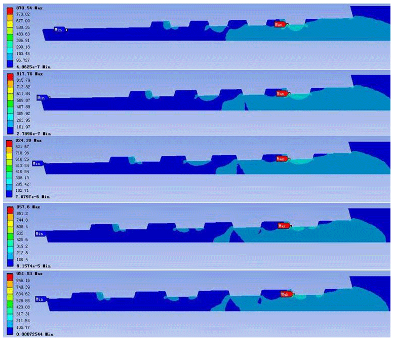
https://www.geosci-instrum-method-data-syst.net/9/79/2020/gi-9-79-2020-f16

Figure 16The stress nephogram of the external thread of the confining probe joint (the pitches from top to bottom are 6, 7, 8, 9, and 10 mm).

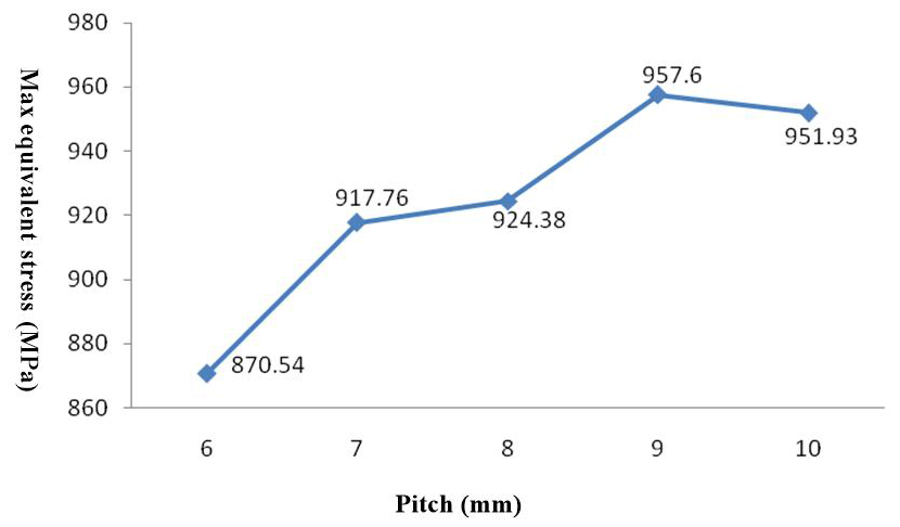
https://www.geosci-instrum-method-data-syst.net/9/79/2020/gi-9-79-2020-f17

Figure 17The trend diagram of the maximum equivalent stress of tube body with pitch increases.

Download

From the finite element analysis results (Fig. 17), the connection strength of the pressure probe tube gradually decreases with the increase of the pitch, and the maximum drop rate is reduced to 90.9 %. In practical applications, the smaller the pitch, the greater the number of thread buckles needed, and the labor intensity of the shackle buckle is increased. Therefore, the pitch should be 8 mm for consideration for comprehensive analysis.

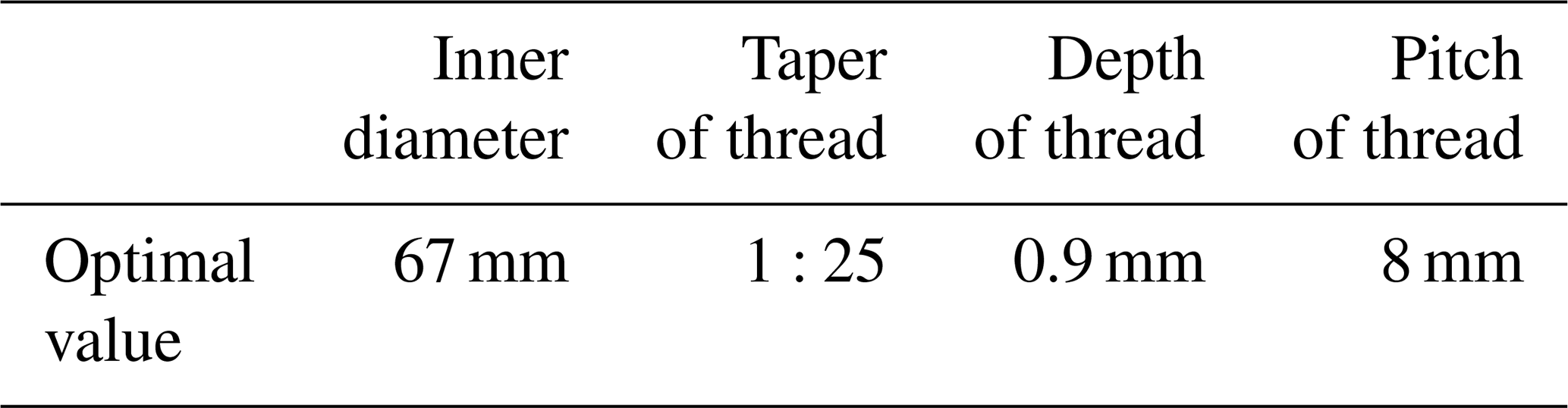
In summary, from the pressure field simulation analysis of the pressure probe, the optimized parameters for the pressure probe and its thread are shown in Table 4.

Table 4Optimized parameters of the pressure probe and its thread.

Download Print Version | Download XLSX

3.2 Metal vacuum flask

Due to the in borehole limitations, the metal vacuum flask is designed with a cylindrical structure. The protected measuring probe is loaded into the flask. As shown in Fig. 18, the metal vacuum flask is mainly composed of a vacuum-insulated bottle, heat absorbers, and a heat insulator.

https://www.geosci-instrum-method-data-syst.net/9/79/2020/gi-9-79-2020-f18

Figure 18Structural diagram of the metal vacuum flask.

Download

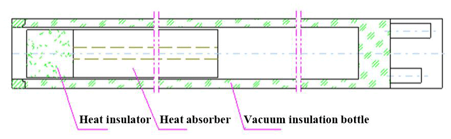
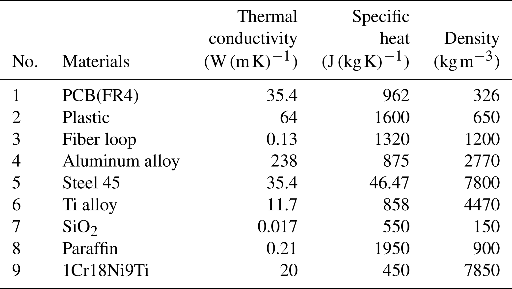
The metal vacuum flask consists of a gland, a plug, a heat-insulating tube, an upper heat absorber, a bottle body (vacuum), a medium heat absorber, and a lower heat absorber. These components are mainly composed of aluminum alloy, 1Cr18Ni9Ti, titanium alloy, and 45 steel. In the process of temperature simulation of the complete fiber-optic gyroscope, the parameters of the relevant materials should be determined (Fang, 2002). The bottle body uses 1Cr18Ni9Ti as the inner shell material, similar to the heat preservation cup, and the material adopts vacuum structure. The heat absorber is mainly made of paraffin, and the heat absorption process is realized by a solid- to liquid-phase transformation. Accounting for the heat from the fiber-optic gyroscope movement and the external temperature, the length of the phase change body is designed; the insulator is made of SiO₂ fiber-reinforced aerogel material. The specific parameters are shown in Table 5.

Table 5Material property parameters of various materials of the metal vacuum flask.

Download Print Version | Download XLSX

3.2.1 Heat calculation in the flask

The heat calculation in the flask consists of the following three parts: heat power calculation of internal measuring components (including FOGs, accelerometers, acquisition board, navigation solution board, data storage output board, and high-temperature battery); calculation of the leakage heat of the flask; and calculation of the heat storage (endothermic). In the trajectory measurement process of the DTMI, the total heat calculation formula is shown in Eq. (4), and the specific calculation is as follows.

\begin{matrix} (4) & \begin{aligned} Q_{Total} & = Q_{Battery - dissipation} + Q_{IMU} - Q_{Absorber} \\ - Q_{Self-dissipation} \end{aligned} \end{matrix}

(a) Heat power calculation of internal measuring components

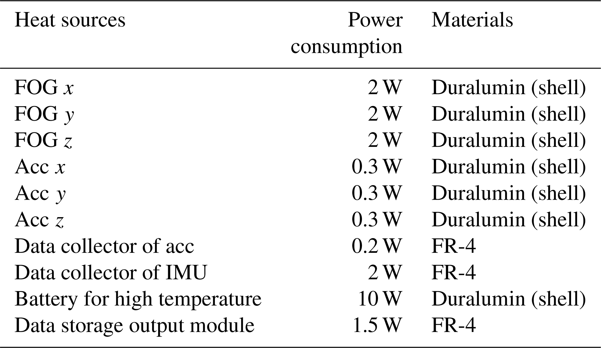
When the DTMI is energized, the entire measurement system (three-axis FOG and three-axis accelerometer) is in a moving state. The orientation of each FOG and accelerometer changes under different moving states. We assume that one hot surface is up, one is down, and one is vertical during the convection process. When the inertial measurement unit is working, the related components will generate heat and compensate for the internal and external temperature difference, so the internal and external temperature differences are not considered. The power consumptions of the main heat sources are shown in Table 6.

Among them, the battery conversion efficiency is assumed to be 80 %, and the rest is converted into heat; Q_IMU is the sum of the power consumptions of the three-axis FOG, the accelerometer, and the circuit board, which is calculated by Eq. (5), where t=4 h and P=21 W.

\begin{matrix} (5) & Q_{IMU} = P \cdot t \end{matrix}

(b) Calculation of leakage heat

The heat leakage of the metal flask is mainly the heat transfer from the outside to the inside, which includes two aspects: (1) axial heat transfer through the flask mouth, including solid heat conduction of the inner tube wall and the heat-insulating plug; (2) radiation leakage between the inner and outer tubes, heat conduction of residual gas, and solid heat transfer between the vacuum layers. The total leakage heat flow rate is set to Φ_sum, Φ₁ is the heat conduction of inner wall of the flask, Φ₂ is the leakage of the heat-insulation plugging, Φ₃ is the radiation leakage heat, and Φ₄ is the residual gas leakage heat. It follows that the total heat leakage Φ_sum is calculated from Φ₁, Φ₂, Φ₃, and Φ₄. The calculation formulas are shown in Eqs. (6) and (7) (Malatip et al., 2012).

\begin{array}{l} (6) & Φ_{sum} = Φ_{1} + Φ_{2} + Φ_{3} + Φ_{4} \\ (7) & \{\begin{cases} Φ_{1} = \frac{A}{L} \cdot \overline{λ} \cdot Δ T \\ Φ_{2} = \frac{S}{L} \cdot \overline{λ} \cdot Δ T \\ Φ_{3} = σ_{0} \cdot A \cdot [{(T_{1})}^{4} - {(T_{2})}^{4}] \cdot \frac{ε_{1} \cdot ε_{2}}{ε_{1} + ε_{2} - ε_{1} \cdot ε_{2}} \cdot \frac{1}{n + 1} \\ Φ_{4} = K \cdot a \cdot P \cdot (T_{1} - T_{2}) \cdot A, \end{cases} \end{array}

where A is the effective cross-sectional area, in m²; L is the length of the thermal conduction section, in meters; ΔT is the temperature difference, taken as 200 K; $\overline{λ}$ is the average thermal conductivity of the material, which is 0.045; the blackbody radiation constant is $5.67 \times 10^{- 8}$ , in ${Wm}^{- 2} K^{- 4}$ ; A is the radiation area, in m²; ε is the effective emissivity, taken as 0.08; T₁ and T₂ are the temperatures of the high- and low-temperature surfaces, respectively, in K; n is the number of layers. When the vacuum is $> 10^{- 3}$ Pa, the residual gas leakage heat can be neglected, so a total leakage heat flux Φ_sum=3.525 W is calculated.

(c) Calculation of heat storage

The heat storage material uses the sensible heat and latent heat of paraffin (phase transition temperature is 60 ^∘C, density is 900 kg m⁻³) to store heat, and the material itself is used to control the rise of external temperature (Fang, 2002). The length of the heat absorber is set to 450 mm, and the heat storage capacity calculated is 101.736 W; when the temperature inside the bottle rises to 125 ^∘C, the heat absorption time is equal to heat storage/total heat leakage flow, so the total endothermic time is calculated as 8.12 h.

Table 6The heat consumption table of main heat source.

Download Print Version | Download XLSX

In summary, the theoretical calculation of the heat in the flask proves that when paraffin wax is used as the heat-absorbing material and its length is designed to be 400 mm, the temperature rise inside flask is guaranteed to be ≤125 ^∘C in a period greater than 7 h.

3.2.2 Simulation and calculation of temperature field

The initial temperature of the internal measuring component was set to 25 ^∘C, the initial temperature of the outer boundary of the metal thermos was set to 270 ^∘C, and the third boundary condition (100) of heat transfer was selected in order to obtain the temperature simulation result, shown in Fig. 19.

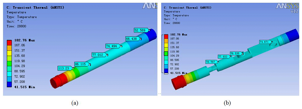
https://www.geosci-instrum-method-data-syst.net/9/79/2020/gi-9-79-2020-f19

Figure 19(a) Temperature distribution nephogram of the metal vacuum flask after 4 h of work; (b) temperature distribution nephogram of the FOG measurement probe after 4 h of work.

Figure 19a is a temperature distribution nephogram of the metal flask after 4 h of working. It can be seen that the overall trend of temperature change in the thermos bottle is gradually reduced from the bottle head to the bottom of the bottle. At the mouth of the bottle, the maximum temperature reaches 113.23 ^∘C, which meets the design requirements (temperature rise <125 ^∘C in flask). Figure 19b is a temperature distribution nephogram of the FOG measurement probe. It can be seen that the internal temperature gradually decreases from the bottle head to the bottom of the bottle, and the temperature values of the different sensor positions are also different. The temperature value on the bottommost FOG is the lowest, which proves the importance of the metal thermos bottle to the temperature rise control of the fiber-optic gyroscope, which is also a guarantee for the measurement accuracy of the FOG.

3.3 Analysis of coupling effect of temperature field and pressure field

In this section, the temperature field–pressure field coupling effect is taken into consideration. Through finite element analysis, a stress and strain distribution, a cloud diagram for the whole measuring instrument is obtained. The deformation state of the outer tube, under the coupling of the temperature field and the pressure field, is analyzed and used to verify the resistance to high temperatures and compression.

Firstly, we simplify the mechanical model of the DTMI; then the coupling of the temperature field and the pressure field is solved by the following three steps: (1) apply temperature boundary conditions, setting the temperature to 270 ^∘C, solve the temperature field, and introduce the temperature field results into statics structural analysis; (2) in static structural analysis, apply a confining pressure load of 120 MPa and constrain it; (3) solve the coupling between the temperature field and the pressure field, as shown in Figs. 20 and 21.

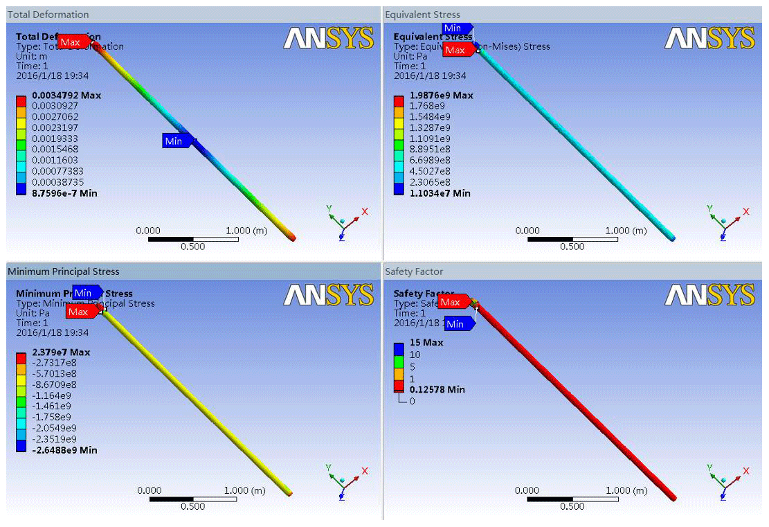
https://www.geosci-instrum-method-data-syst.net/9/79/2020/gi-9-79-2020-f20

Figure 20The stress nephogram of the coupling between the temperature field and the pressure field: the upper left is the total deformation nephogram; the upper right is the equivalent strain nephogram; the lower left is the minimum principal stress nephogram; the lower right is the Mohr–Coulomb stress displacement safety factor nephogram.

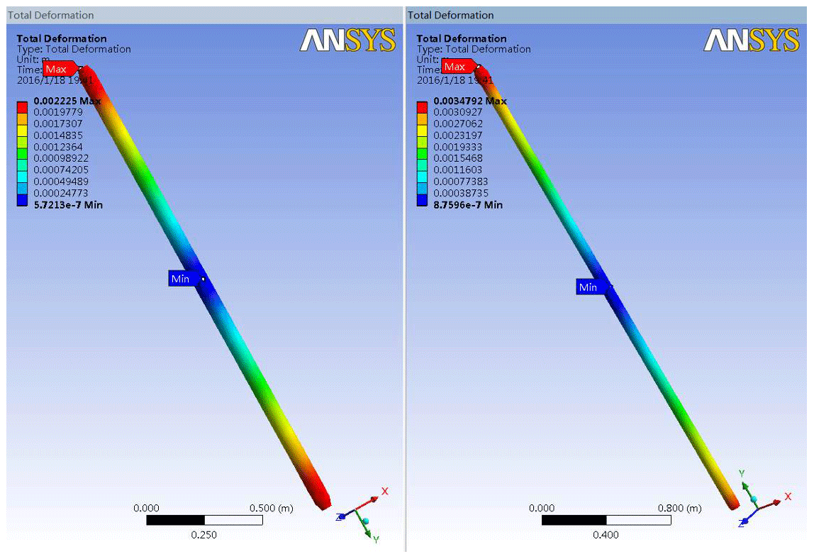
https://www.geosci-instrum-method-data-syst.net/9/79/2020/gi-9-79-2020-f21

Figure 21The total deformation nephogram comparison: the left picture shows the pressure field total deformation nephogram; the right picture shows the pressure field and temperature field coupling total deformation nephogram.

Analysis of the finite element results shows that under the action of high temperature and high pressure, the total deformation of the DTMI increases and the equivalent strain increases, when compared with the action of the pressure field alone. The maximum deformation of the DTMI is calculated to be 3.47 mm m⁻¹. The deformation is 1.33 mm, which meets the requirement that the deformation amount per 1 m in the parameter index should be less than 1.5 mm.

3.4 FOG error analysis and compensation in temperature field

Due to thermal field distribution and heat transfer under the thermal transient state, the physical properties, geometrical features, and thermal transfer of the FOG are dynamically changing over time, leading to a Shupe error in the FOG inclinometer. The Shupe error is negatively correlated to the accuracy of the inclinometer. To enhance the accuracy of the IMU, the finite element method (FEM) was adopted to analyze the heat conduction features of the inclinometer in a thermal field. This method can overcome the limits of traditional analytical techniques. For instance, it can handle the complex boundary conditions of the FOG. According to the differential control equations for heat conduction, a FOG error compensation formula in thermal field was derived through Shupe error analysis, laying the basis for FOG thermal field modeling and error compensation.

3.4.1 Shupe error analysis

In the thermal transient state, the Shupe error can be calculated based on the phase delay ϕ of the light wave propagation in a fiber loop with length L (Mohr, 1995):

\begin{matrix} (8) & ϕ = \int_{0}^{L} β (z) d z = \int_{0}^{L} β_{0} n (z) d z, \end{matrix}

where β₀ is the propagation constant of light in free space; n(z) is the refractive index. Since the thermal expansion and refractive index of the medium may vary with the temperature fields during light wave propagation, Eq. (8) can be rewritten as Eq. (9):

\begin{matrix} (9) & ϕ = β_{0} n_{eff} L + β_{0} (\frac{\partial n_{eff}}{\partial T} + n_{eff} α) \int_{0}^{L} Δ T (z) d z, \end{matrix}

where n_eff is fiber refractive index; ( $\partial_{neff}) / \partial_{T}$ is the temperature coefficient; α is fiber thermal expansion coefficient; ΔT(z) is the temperature change. Using the Sagnac effect, the FOG measures the phase difference of two beams of a light wave through the same optical fiber with length L. One beam of light wave propagates in the clockwise direction, and the other in an counter-clockwise direction. Specifically, the clockwise phase delay ϕ_cw(t) and the counter-clockwise phase delay ϕ_ccw(t) are calculated, and the Shupe error Δϕ_E(Shupe) in the thermal transient state is given a differential time definition (Raab and Quast, 1994). The Δϕ_E(Shupe) can be calculated by

\begin{matrix} (10) & Δ ϕ_{E} (Shupe) = \frac{β_{0}}{c_{m}} (\frac{\partial n_{eff}}{\partial T} + n_{eff} α) \int_{0}^{L} \dot{T} (z, t) (L - 2 z) d z, \end{matrix}

where $\dot{T} (z, t)$ is the temperature change rate in the fiber loop $(\dot{T} (z, t) = \partial T / \partial z)$ . Equation (10) shows that the Shupe error reflects how the temperature gradient affects the FOG measuring accuracy. To sum up, the Shupe error Δϕ_E(Shupe), induced by the temperature field variation in the transient state, has a certain effect on the output light intensity, I, of the FOG in that it reduces the measuring accuracy of FOG inclinometer. The output light intensity, I, can be obtained as follows:

\begin{matrix} (11) & I = I_{0} \{1 + \cos [ϕ_{S} + Δ ϕ_{S} (Shupe)]\} . \end{matrix}

3.4.2 Error compensation formula of FOG in the temperature field

Under the joint action of Shupe error Δϕ_E(Shupe) and the additional phase shift ϕ_ΔL in the transient state, an error will occur in the Sagnac phase shift ϕ_S. Based on the previous analysis of Shupe error, this section attempts to deduce the error formula in the thermal transient state and then the FOG error compensation formula in the temperature field.

Due to the temperature field and the thermal stress in the FOG, the fiber loop length L changes by a certain degree. Hence, $L / d ≫ 1$ , with d being the diameter of the fiber. By the definition of the thermal expansion coefficient (Sokolov et al., 2015), the thermal expansion coefficient α of the optical fiber in the thermal transient state can be expressed as

\begin{matrix} (12) & α = \frac{d (Δ z)}{Δ z \cdot d [T (z, t)]} . \end{matrix}

In Eq. (12), z is a point on the optical fiber loop of the FOG. Then, the linear deformation of the fiber loop ΔL leads to a Sagnac equivalent phase shift ϕ_ΔL:

\begin{array}{l} (13) & ϕ_{Δ L} = Δ L \cdot \frac{\partial ϕ_{S}}{\partial L} = Δ T \cdot α \cdot L \cdot \frac{\partial ϕ_{S}}{\partial L} \\ (14) & Δ ϕ_{S} (Δ L) = α \cdot \frac{\partial ϕ_{S}}{\partial L} \cdot \sum Δ T (z, t) \cdot Δ z . \end{array}

It can be seen that Δϕ_S(Shupe) in the thermal transient state is correlated with the linear expansion coefficient, α, and effective refractive index, n_eff, of the optical fiber: $Δ ϕ_{S} (Shupe) = F (α, \dots, n_{eff})$ . Then, Eqs. (13) and (14) are derived by finding the partial derivatives of α and n_eff, and Eqs. (13) and (14), respectively, depict the effect of the Sagnac phase shift in thermal transient state caused by the linear deformation and refractive index variation of the optical fiber; the linear expansion coefficient, α, is determined by the material of the fiber.

\begin{array}{l} (15) & \frac{\partial [Δ ϕ_{S} (Shupe)]}{\partial α} & = \frac{β_{0}}{c_{m}} \cdot n_{eff} \cdot \int_{0}^{L} \dot{T} (z, t) (L - 2 z) d z \\ \frac{\partial [Δ ϕ_{S} (Shupe)]}{\partial α} & = (\frac{α β_{0}}{c_{m}} + \frac{\partial (\frac{\partial n_{eff}}{\partial T})}{\partial n_{eff}}) \\ (16) & \cdot \int_{0}^{L} \dot{T} (z, t) (L - 2 z) d z \end{array}

On the premise of using the same material fiber, and combining this with Eqs. (10), (15), and (16), error theory analysis shows that the factors affecting the Shupe error of the FOG in a thermal field are mainly the temperature change rate, the effective refractive index, and the angular velocity. Therefore, these formulas serve as the guide for FOG error compensation in a thermal field, effectively paving the way for a rational error compensation plan.

4 Engineering application

4.1 Engineering application in the CCSD SK-2 east borehole

4.1.1 CCSD SK-2 east borehole

The CCSD project in the Songliao Basin aimed to investigate deep geothermal energy, establish a deep stratigraphic structure profile, seek geological evidence of Cretaceous climate change, and develop deep detection techniques. This was the third international CCSD project funded by the China Mainland Scientific Drilling Program (ICDP) (Wang et al., 2013, 2017). As the main borehole of this project, the SK-2 east borehole was designed to reach a depth of 6400 m, in order to penetrate the Cretaceous strata and reach the base of the basin. It is located about 0.25 km southeast of Jiqing village, Yangcao town, Anda city, Heilongjiang province (Zou et al., 2016; Zhu et al., 2018). The main scientific objectives of logging the CCSD SK-2 east borehole are (1) to provide complete and continuous petrophysical parameters and well-side structural parameters for use in the establishment of a Cretaceous continental sedimentary study at the geophysical exploration “scale”; (2) to explore the relationship between the global greenhouse climate and environmental changes using logging information during the Cretaceous period from 65 million to 140 million years; (3) to carry out reservoir division and oil and gas evaluation for key hydrocarbon-bearing horizons; (4) to provide the basic information necessary for the full-scale long-term observation and experimental research of the CCSD SK-2 east borehole in the future (Xu, 2004; Gao et al., 2015; Zou et al., 2018).

Geophysical logs played an important role in the subsequent geoscience research because very few core samples were recovered over the Upper Cretaceous intervals (i.e., Spud 1 and Spud 2). After the borehole was drilled, just two uncased and cased borehole logging operations (using Beck Atlas' ECLIPS-5700 and Halliburton's EXCEL 2000) were carried out in the Upper Cretaceous intervals using advanced imaging logging tools (Zou et al., 2016). Therefore, DTMI's engineering application was selected for the SK-2 east borehole to test the performance in the high temperature and high pressure of the scientific detection wells, and to test the startup performance and overall performance of the power supply in the low-temperature field environment (the ambient surface temperature is about −2 ^∘C at the SK-2 east borehole).

4.1.2 Testing steps

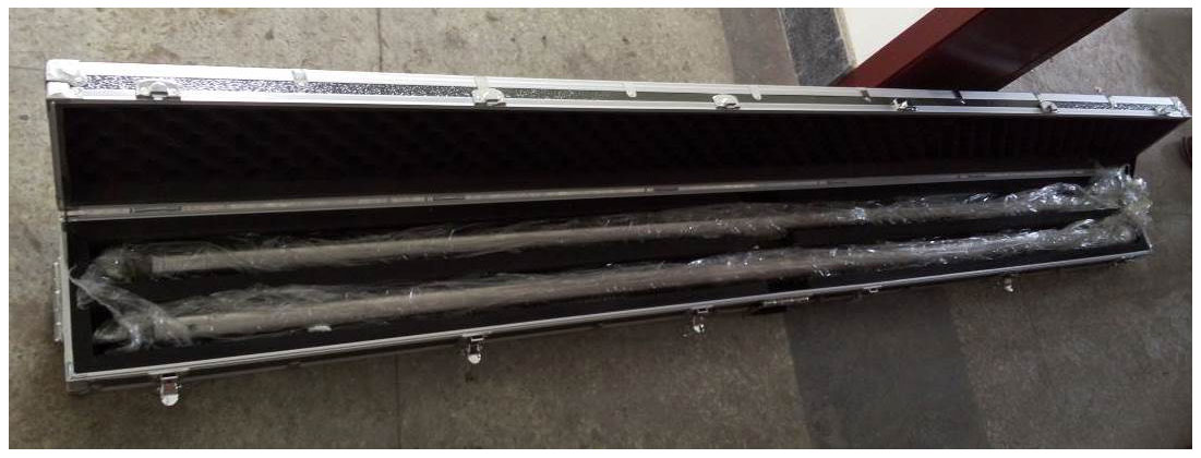
The engineering application time was on 15–16 October 2017. At that time, the construction depth of the SK-2 east borehole had exceeded 6200 m, the depth of the casing was 5905 m, the specific gravity of the mud was 1.46, and the pressure of the mud column at the bottom of the well exceeded 90 MPa. The bottom temperature exceeded 200 ^∘C. Under the suggestion of the construction party, the application test was carried out in the casing section, using two DTMIs at the same time, and the measurement was carried out at intervals of 500 m. A photo of the DTMI used in this engineering application is shown in Fig. 22.

https://www.geosci-instrum-method-data-syst.net/9/79/2020/gi-9-79-2020-f22

Figure 22Photo of DTMI which applies to the SK-2 east borehole.

Download

The main contents of the engineering application were three methods: a closed water test, downward trajectory measurement, and upward trajectory measurement. The purpose was to test the sealing, pressure, thermal insulation performance, and reliability of the measurement data of the DTMI.

The closed water test is a pilot test to verify the sealing performance of the pressure probe and to investigate the inside of the hole. In order to prevent the core measuring component, based on the FOG, from being damaged due to seal failure, when the water shutoff test was carried out, the FOG movement was not placed in the pressure probe tube. Instead, a humidity test paper and a boiling point thermometer were placed in the tube. After the water shutoff test was completed, the measuring device was taken out and the pressure and sealing ring of the pressure-reducing probe were verified to be non-destructive, the inside of the pressure-exploring probe was dry, and the humidity test paper showed no obvious changes. This indicated that the pressure-exploring tube had good sealing performance and could meet the design requirements.
When preparing for measurements in the borehole, raw tape was wrapped on the connecting threaded joint and thread oil was applied to protect the thread and further improve the sealing performance; then the downward measurement was started, and the DTMI was lowered through the wire rope, or cable, of the ground gauge winch; after reaching the bottom of the hole, the upward measurement was started, and the measured data were stored in the memory of the probe; after the trajectory measurement process was finished, the internal measurement probe was taken out of the confining tube and metal flask; finally, the movement probe was connected to the PC using a data line and a conversion joint, and the trajectory measurement data stored in the movement were read. Then, data acquisition and processing were performed, thereby obtaining data on the drilling trajectory.

4.1.3 Data analysis

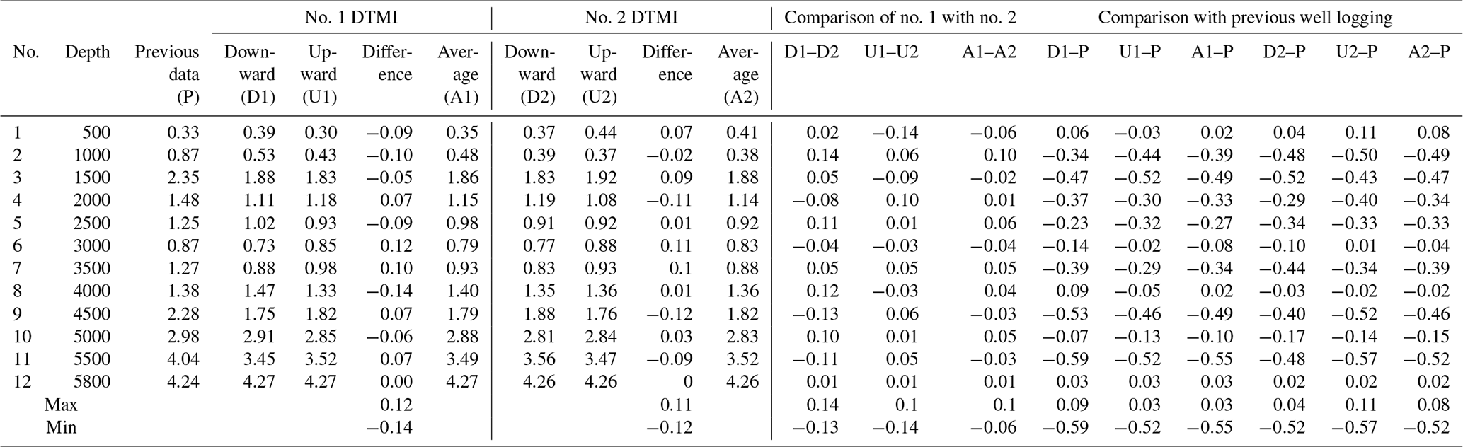
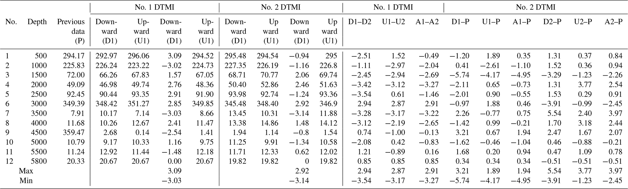
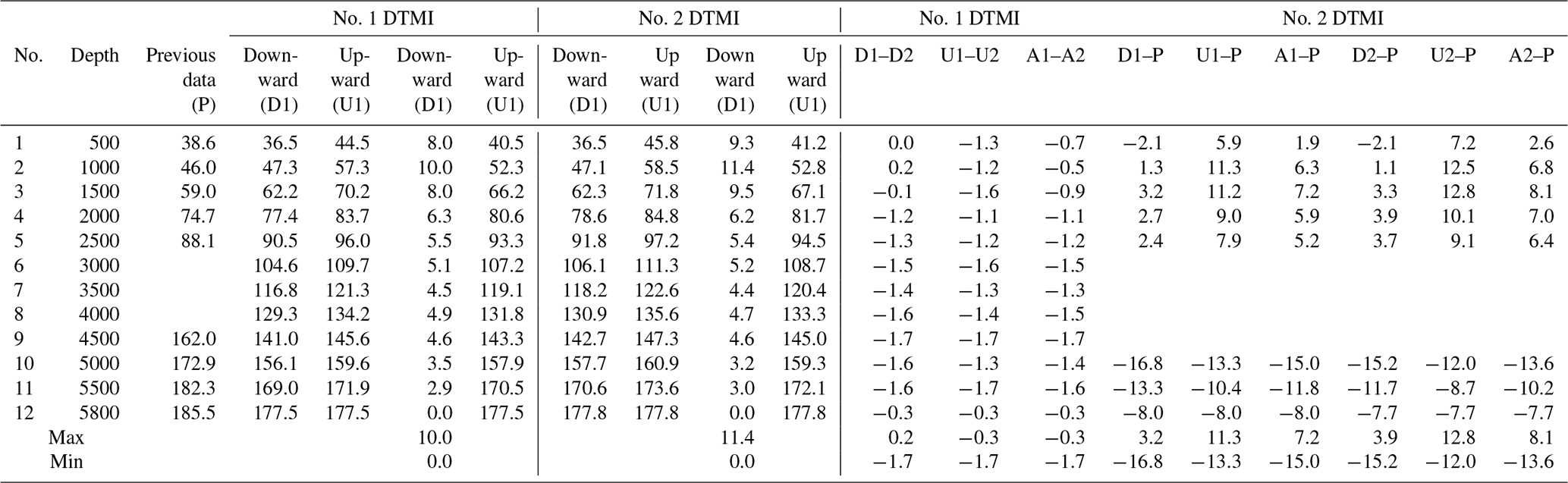
The maximum well depth for this measurement was 5800 m, and the highest temperature measured was 177.8 ^∘C. The detailed measured data of zenith angle, azimuth angle, and temperature are shown in Tables 7, 8, and 9. The comparative analysis of the measured data gave the following results:

Table 7Measured zenith angle of the CCSD SK-2 east borehole.

Download Print Version | Download XLSX

Table 8Measured azimuth angle of the CCSD SK-2 east borehole.

Download Print Version | Download XLSX

Table 9Measured azimuth angle of the CCSD SK-2 east borehole.

Download Print Version | Download XLSX

The zenith between the downward and upward measurements of one DTMI and between the two sets of DTMIs were in good agreement with each other. The result had good repeatability, with an error less than 0.15^∘.
When the zenith was less than 3^∘, the error of the azimuth data between the downward and upward measurements of one DTMI and between the two sets of DTMIs was relatively large. When the zenith was greater than 3^∘, the error of the azimuth data between downward and upward measurements of one DTMI and between the two sets of DTMIs was less than 0.15^∘.
In the process of downward and upward measurements, the temperature-measured data of the two sets of instruments were consistent with each other.
The two sets of the DTMI-measured data for zenith and azimuth were compared with previous logging data. We found that the data were roughly consistent with each other, although there were certain deviations in individual points. The main reason for these deviations in the data may be that the previous logging data were measured in the open well, while this measurement was done after the casing was placed in the well. The data deviation was normal, and its accuracy is acceptable for deep exploration engineering and underground resources and energy engineering.
There was a deviation in the temperature data between the downward and upward measurements, mainly due to the short time of the measurement at each point (except for 5 min at the well bottom, at 5800 m; the other measurement points were occupied for only 30 s), and there was a failure of the heat to sufficiently stabilize at the temperature sensor.
The deviation between the measured temperature value at 5800 m and the previous logging data was due to the fact that the logging data were in the open well and the original temperature waiting time reached 30 min. Here, the measurement was in the casing and the waiting time was only 5 min. Thus, the temperature sensor had not reached a temperature balance with the bottom of the well environment.

Figure 23a shows a curve of measured zenith against borehole depth, Fig. 23b shows a curve of measured azimuth against borehole depth, and Fig. 23c shows a curve of measured temperature against borehole depth.

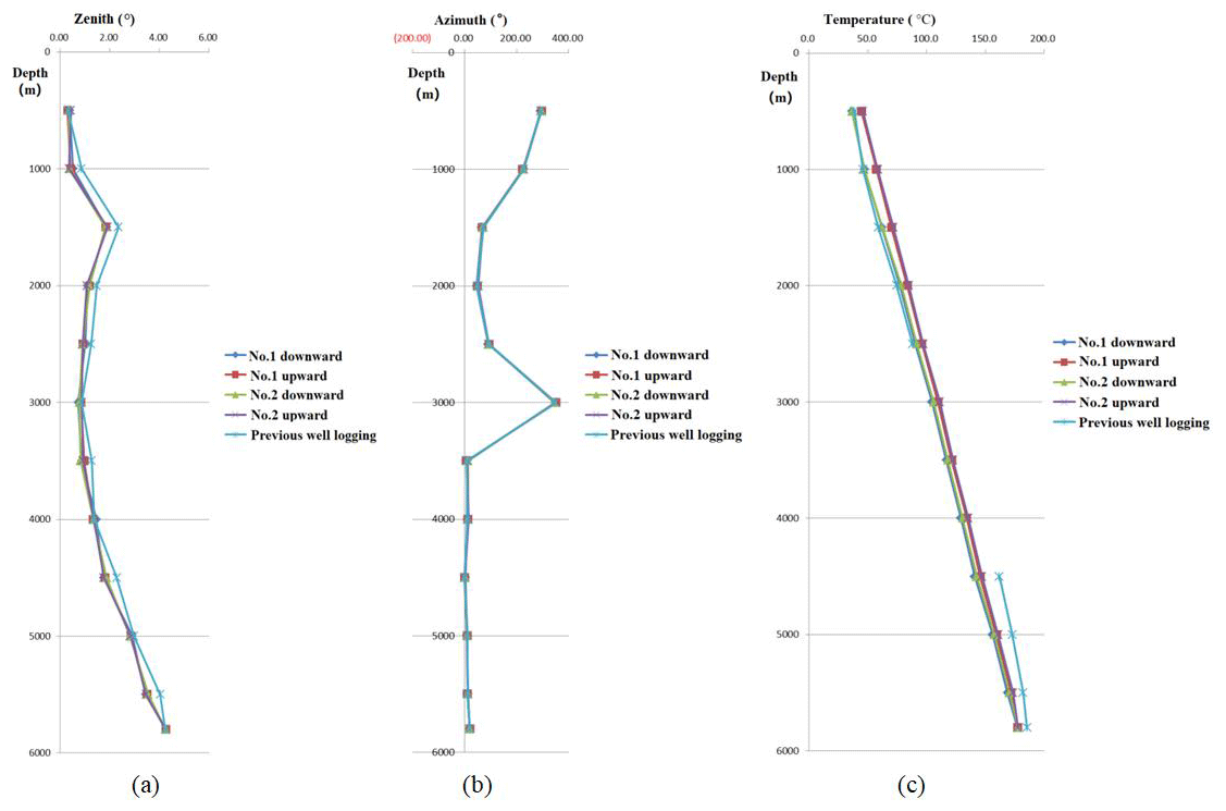
https://www.geosci-instrum-method-data-syst.net/9/79/2020/gi-9-79-2020-f23

Figure 23(a) Curve of measured zenith against borehole depth; (b) curve of measured azimuth against borehole depth; (c) curve of measured temperature against borehole depth.

Download

4.2 Engineering application in the geothermal well of Xingreguan-2, Beijing

4.2.1 Geothermal well of Xingreguan-2

The Xingreguan-2 well is a geothermal well within the dolomite formation of the Wuyishan Formation, in Jixian county. It is located in the Xingming Lake Resort in the Daxing district, Beijing. The well location coordinates are latitude 39^∘36^′48.09^′′ and longitude 116^∘25^′56.54^′′ (Zhao, 2011). The well is a geothermal well within the dolomite group of the Wuyishan Formation. It was drilled for the water intake section on 31 May 2016. The completion depth is 2505.18 m, the water output is 1549.67 m³ d⁻¹, and the wellhead outlet temperature is 46 ^∘C. The application time was from 14:00 to 17:00 UTC+8 on 14 November 2017, and one DTMI was used for this measurement. In order to ensure the safety of the instrument and avoid the measurement of bare holes, the depth of this measurement was only 1750 m; during decentralization and lifting of the instrument, measurements were made at the same depths of the well, with intervals of 200 m.

4.2.2 Data analysis

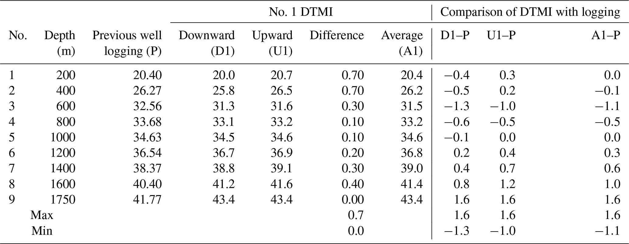
The maximum well depth for this measurement was 1750 m, and the highest temperature measured was 43.4 ^∘C. The detailed measured data of the zenith angle, azimuth angle, and temperature are shown in Tables 10, 11, and 12. The comparative analysis of the measured data gave the following results:

Table 10Measured zenith angle of the Xingreguan-2 well, Beijing.

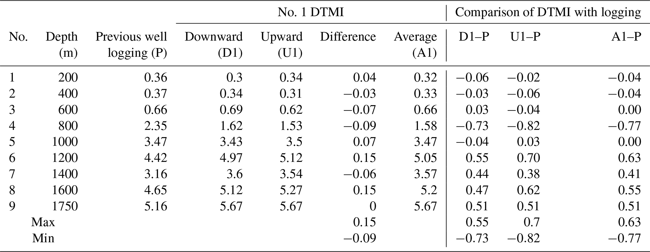
Download Print Version | Download XLSX

Table 11Measured azimuth angle of the Xingreguan-2 well, Beijing.

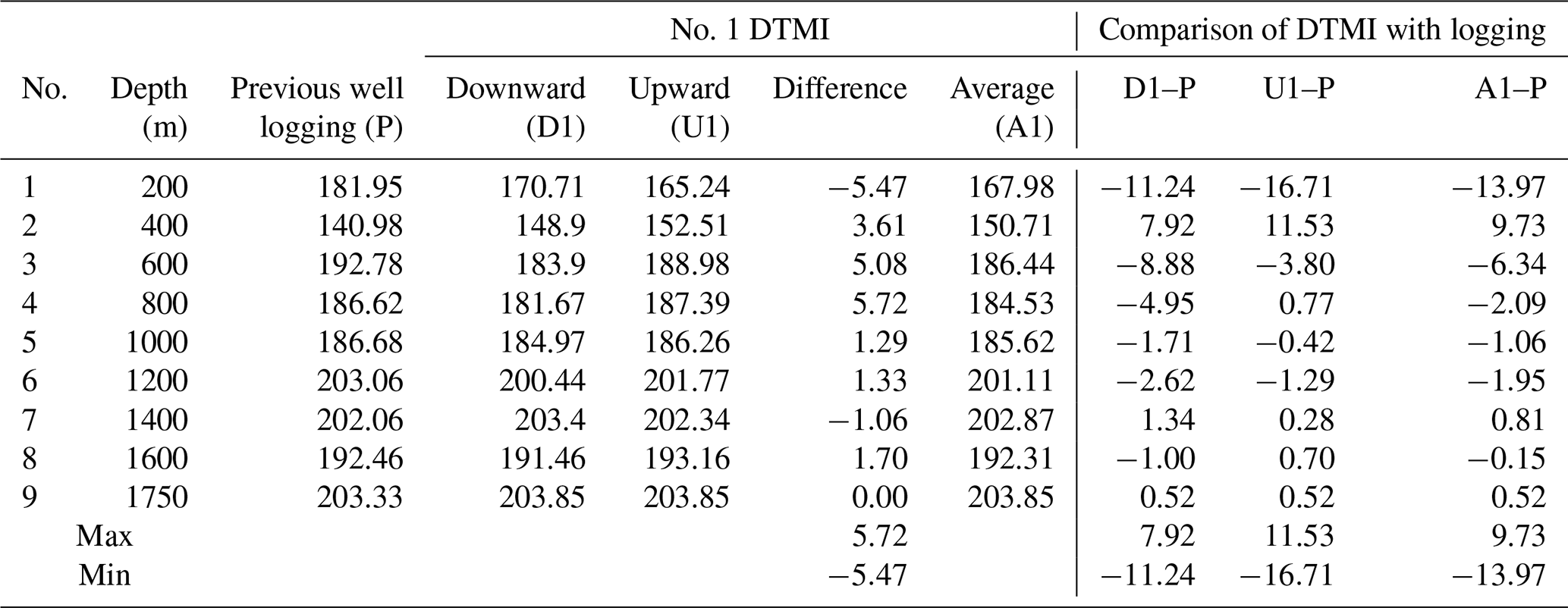
Download Print Version | Download XLSX

Table 12Measured temperature of the Xingreguan-2 well, Beijing.

Download Print Version | Download XLSX

The zenith angles between downward and upward measurements were in good agreement with each other, and the result showed good repeatability, with an error of less than 0.15^∘; when the zenith was less than 3^∘, the error of the azimuth data between the downward and upward measurements was relatively large and when the zenith was greater than 3^∘ (for the measuring points at 1000, 1200, 1400, 1600, and 1750 m depth), the error of the azimuth data between downward and upward measurements was less than 0.15^∘
In the process of downward and upward measurements, the temperature-measured data of the two sets of instruments were consistent with each other.
The DTMI-measured data for zenith and azimuth were compared with previous logging data. We found that the data were roughly consistent with each other, although there were certain deviations at individual points. The main reason for these deviations in the data may be that the previous logging data were measured in the open well and these measurements were done after the casing was placed in the well.

Figure 24a shows a curve of measured zenith against borehole depth, Fig. 24b shows a curve of measured azimuth against borehole depth, and Fig. 24c shows a curve of measured temperature against borehole depth.

https://www.geosci-instrum-method-data-syst.net/9/79/2020/gi-9-79-2020-f24

Figure 24(a) Curve of measured zenith against borehole depth; (b) curve of measured azimuth against borehole depth; (c) curve of measured temperature against borehole depth.

Download

5 Discussion

The FOG has the advantages of high measurement accuracy, small size, high sensitivity, and strong anti-interference ability. This is especially important for the magnetic material with the greatest influence on the trajectory measurement technology in geological exploration and external magnetic field interference. The DTMI, based on the FOG, can be used for borehole trajectory measurements in any formation conditions. The FOG, used in geological and oil drilling fields, generally requires a wide operating temperature range. However, the measurement accuracy of the FOG is very sensitive to changes in ambient temperature, especially in deep borehole testing. The high external temperature and high-pressure environment, along with internal self-heating, will have an impact on the performance of the FOG. This mostly manifests as noise and drift. The noise directly affects the working accuracy of the fiber-optic gyroscope, that is the minimum detectable phase shift, while the drift reflects the degree of change in the output signal. Therefore, the thermal non-reciprocal error (Shupe error) caused by the temperature field will seriously affect the performance of the FOG inclinometer. This is characterized by poor data repeatability, short working time, and low precision (Shupe, 1980; Kurbatov, 2013).

Due to the Shupe error caused by the temperature field of the FOG, it is difficult to carry out thermal simulation analysis of the whole structure and internal mechanism by a traditional thermal field analytical method. It is nearly impossible to determine the boundary range, control equation, and thermal characteristics of the main components (Yang et al., 2011). In this study, the finite element method was used to analyze the heat transfer characteristics of the borehole trajectory measuring instrument. In Sect. 3.3, the Shupe error of the fiber-optic gyroscope was calculated using the differential control equations for thermal conduction and the thermal boundary condition. The unified formula of the thermal error was derived. The external parameters that affect the Shupe error are mainly temperature change rate, the effective refractive index, and the angular velocity. Therefore, these formulas can be used as the basis for the temperature field model establishment and error compensation experimental scheme for the internal core measurement mechanism.

In order to reduce the influence of temperature changes on the output accuracy of the fiber-optic gyroscope, the FOG error compensation experiment was used to establish a temperature compensation model between the parameters (temperature change rate, the effective refractive index, and the angular velocity) and the FOG output value, and to explore the mathematical relationship between them. Coefficients of the model require the FOG measurement probe to be tested on a three-axis quadrature calibration bench with a high-temperature thermostat, thereby obtaining a series of experimental data (Liu et al., 2019); photos of the temperature compensation experiment are shown in Fig. 25.

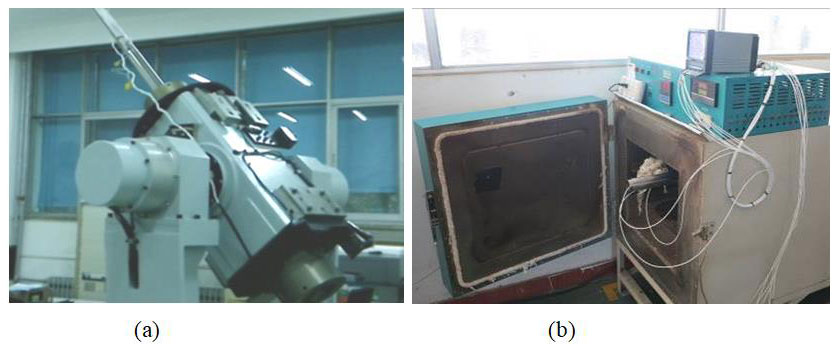
https://www.geosci-instrum-method-data-syst.net/9/79/2020/gi-9-79-2020-f25

Figure 25(a) Photo of the experiments on three-axis quadrature calibration bench; (b) photo of the experiments in high-temperature thermostat.

Download

Due to the higher temperature in boreholes, up to 250 ^∘C, a metal vacuum flask was used to ensure that the internal space did not exceed 125 ^∘C degrees (Liu et al., 2016). The temperature range of the measuring probe was set from 0 to 120 ^∘C in the experiments. There are four influence factors in the FOG error compensation experiments, namely experimental temperature range, temperature change rate, effective refractive index, and angular velocity. Therefore, a four-layer network structure was employed. The parameter values (number of levels) for each factor are shown in Table 13.

Table 13Table of experimental factors and their levels.

Download Print Version | Download XLSX

The thermal error compensation experiments usually employ a network structure of three to four layers (Meng et al., 2009). During these experiments, we found that both full-scale design methods and orthogonal design methods were time-consuming and low in efficiency for FOG error compensation. For example, in the full-scale design method, the number of experiments required is $6 \times 12 \times 4 \times 4 = 1152$ . If an experiment takes 10 min, it will take 192 h to complete the full-scale design method experiments. The time needed for these experiments was not available. Therefore, more advanced experimental protocols should be used to simplify the experimental process, such as the uniform design method, neural network method, and fuzzy mathematics method. As an experimental design for space filling, the uniform design method describes a test point spread evenly throughout the test range and thus has been proposed from the perspective of uniformity (Fang, 1994). In particular, the design enables the conduct of trials with many experimental factors and a large number of levels but with fewer trials required when compared to the orthogonal or comprehensive design methods (Deesuth et al., 2012). Therefore, future work will involve the use of the uniform design method for temperature compensation experiments, establish a neural network dynamic model to compensate its output, improve the FOG temperature compensation accuracy, and ensure the stability of the DTMI-measured data.

6 Conclusions

A drilling hole trajectory measuring instrument, based on interference FOG, is developed in this study. We examined the mechanical design and strength. We carried out pressure field simulation analysis for the pressure-bearing outer tube. The structural design of the metal thermos was examined, and we carried out temperature field simulation analysis, measuring with the FOG in the probe. The study of Shupe error compensation in the field of temperature field was carried out using finite element analysis, for 4 h, in an environment where the maximum temperature does not exceed 270 ^∘C and the pressure does not exceed 120 MPa. Engineering applications were carried out in the CCSD SK-2 east borehole and the geothermal well of Xingreguan-2. Data such as azimuth, apex angle, and temperature were obtained and compared with results from previous logging equipment. The engineering applications proved that DTMI had good measurement accuracy and repeatability, high stability, and reliable measurement methods.

Aimed at the difficult working conditions in boreholes of hot dry rock, deep geothermal investigation drilling, and ultra-deep geological drilling (up to 5000 m), this instrument is based on the principle of inertia and is not affected by external electrical and magnetic interference. This makes up for the working blind zone of existing technologies and instruments. Therefore, DTMI has great potential for the development and advances in geological drilling technology.

The main highlights of this paper are as follows:

A method for measuring the borehole trajectory based on a three-axis interference-type fiber-optic gyroscope is proposed. The two-axis orthogonal three-axis fiber gyroscope and three-axis accelerometer sensor are used to form the strapdown inertial navigation system. The three-axis displacement and the three-axis rotation angle can be calculated by the trajectory calculation model described in the text. The DTMI can be applied in strong magnetic interference mining areas and expands the scope of engineering applications. Compared with existing drilling trajectory measuring equipment using a fluxgate or single-axis and two-axis gyroscopes as sensitive devices, it is a step forward in novelty and innovation.
The DTMI pressure field–temperature field coupling analysis method is proposed to guide the optimal design of the DTMI. Using a finite element software platform, the DTMI thread parameters, the size and wall thickness of the confined probe, optimization of the material and structure of the metal vacuum flask was carried out, and the simulation analysis and optimization design of the pressure field–temperature field coupling effect for the whole instrument were carried out. Finally, the reliability and stability of the DTMI were verified by the engineering application in the CCSD SK-2 east borehole.

Data availability

The data used to support the findings of this study are available from the corresponding author upon request.

Author contributions

YL and GL designed and built the instrument with the help of CW and WJ. YL and CW prepared the paper with contributions from all authors.

Competing interests

The authors declare that they have no conflict of interest.

Acknowledgements

Ce Zhou and Wenjun Chen helped acquire the data of engineering application presented in this paper; Zhong Li processed the data in Tables 7–9, for which he is gratefully acknowledged.

Financial support

This research has been supported by the National Natural Science Foundation of China (grant no. 41804089); the National Key Scientific Instrument and Equipment Development Project of China (grant no. 2013YQ050791); and the China Postdoctoral Science Foundation (grant no. 2019M650782).

Review statement

This paper was edited by Luis Vazquez and reviewed by two anonymous referees.

References

Bernardo, C. and Shu, C.-W.: TVB Runge–Kutta Local Projection Discontinuous Galerkin Finite Element Method for Conservation Laws II: General Framework, Math. Comput., 52, 411–435, https://doi.org/10.2307/2008474, 1989.

Çelikel, O. and Sametoğlu, F.: Assessment of magneto-optic Faraday effect-based drift on interferometric single-mode fiber optic gyroscope (IFOG) as a function of variable degree of polarization, Meas. Sci. Technol., 23, 25104–25120, https://doi.org/10.1088/0957-0233/23/2/025104, 2012.

Chen, Z., Zheng, K., and Jiang, J.: Discussion on the development strategy of hot dry rock in China, Hydrogeol. Eng. Geol., 43, 161–166, https://doi.org/10.16030/j.cnki.issn.1000-3665.2015.03.26, 2015.

Deesuth, O., Laopaiboon, P., Jaisil P., and Laopaiboon, L.: Optimization of Nitrogen and Metal Ions Supplementation for Very High Gravity Bioethanol Fermentation from Sweet Sorghum Juice Using an Orthogonal Array Design, Energies, 5, 3178–3197, https://doi.org/10.3390/en5093178, 2012.

Fang, K.: Uniform design and uniform design table, Science Press, Beijing, China, 1994.

Fang, K.: Materials engineering handbook, Beijing Press, Beijng, China, 2002.

Gao, W., Kong, G. Pan, H. et al.: Geophysical logging in scientific drilling borehole and find deep Uranium anomaly in Luzong basin, Chinese J.. Geophys., 58, 4522–4533, https://doi.org/10.6038/cjg20151215, 2015 (in Chinese with English abstract).

Grewal, M. S., Weill, L. R., and Andrews A. P.: Global Positioning System, Inertial Navigation, and Integration, Wiley Int. Rev. Comput. Stat., 3, 383–384, https://doi.org/10.1002/wics.158, 2007.

Kielbassa, A. M., Fuentes, M. D., Goldstein, M., and Arnhart, C.: Randomized controlled trial comparing a variable-thread novel tapered and a standard tapered implant: Interim one-year results, J. Prosthet. Dent., 101, https://doi.org/10.1016/S0022-3913(09)60060-3, 293–305, 2009.

Kurbatov, A. M. and Kurbatov, R. A.: Temperature characteristics of fiber-optic gyroscope sensing coils, J. Commun. Technol. El., 58, 745–752, https://doi.org/10.1134/S1064226913060107, 2013.

Liu, Y.: Design of the Drilling Trajectory Measurement Device in Ultra-high Temperature based on FOG and Its Key Technologies Research, PhD thesis, Sichuan university, Chengdu, China, 2016.

Liu, Y., Wang, J., Ji, W., and Luo, G.: Temperature Field Finite Element Analysis of the Ultra-high Temperature Borehole Inclinometer based on FOG and Its Optimization Design, Chem. Eng. Trans., 51, 709–714, https://doi.org/10.3303/CET1651119, 2016.

Liu, Y., Wang, C. Wang, J., and Ji, W.: Optimization Research on Thermal Error Compensation of FOG in Deep Mining using Uniform Mixed-data Design Method, Math. Probl. Eng., 2019, 1–6, https://doi.org/10.1155/2019/4064652, 2019.

Maas, S. J. and Metzbower, D. R.: Optical accelerometer, optical inclinometer and seismic sensor system using such accelerometer and inclinometer: US Patent 7,222,534. 29 May 2007.

Malatip, A., Wansophark, N., and Dechaumphai, P.: Fractional four-step finite element method for analysis of thermally coupled fluid-solid interaction problems, Neuropharmacology, 33, 253–257, https://doi.org/10.1007/s10483-012-1536-9, 2012.

Meng, Y., Chen, Y., Li, S., Chen, C., Xu, K., Ma, F., and Dai X.: Research on the orthogonal experiment of numeric simulation of macromolecule-cleaning element for sugarcane harvester, Mater. Design, 30, 2250–2258, https://doi.org/10.1016/j.matdes.2008.08.020, 2009

Mohr, F.: Thermooptically Induced Bias Drift in Fiber Optical Sagnac Interferommeters, Lightwave Technol., 14, 27–41, https://doi.org/10.1109/50.476134, 1995.

Osipova, E. N., Ivanov, I. V., Smirnov, V. A., and Abramova, R. N.: Terrestrial heat flow and its role in petroleum geology, Earth Environ. Sci., 27, 12–15, https://doi.org/10.1088/1755-1315/27/1/012015, 2015.

Raab, M. and Quast, T.: Two-color Brillouin Ring Laser Gyro with Gyrocompassing Capability, Opt. Lett., 19, 1491–1496, https://doi.org/10.1364/OL.19.001492, 1994.

Savage, P. G.: Blazing Gyros: The Evolution of Strapdown Inertial Navigation Technology for Aircraft, J. Guid. Control Dynam., 36, 637–655, https://doi.org/10.2514/1.60211, 2013.

Sedlak, V.: Magnetic pulse method applied to borehole deviation measurements, Int. J. Rock Mech. Min., 39, 61–75, https://doi.org/10.1016/0148-9062(95)99588-O, 1994.

Shupe, D. M.: Thermally induced nonreciprocity in the fiber-optic interferometer, Appl. Optics, 19, 654–655, https://doi.org/10.1364/AO.19.000654, 1980.

Sokolov, A. V., Krasnov, A. A., Staroseltsev, L. P., and Dzyuba, A. N.: Development of a gyro stabilization system with fiber-optic gyroscopes for an air-sea gravimeter, Gyrosc. Navi., 6, 338–343, https://doi.org/10.1134/S2075108715040124, 2015.

Tavio, T. and Tata, A.: Predicting Nonlinear Behavior and Stress-Strain Relationship of Rectangular Confined Reinforced Concrete Columns with ANSYS, Civil Eng. Dim., 11, 123–129, 2009.

Titterton, D. and Weston, J.: Strapdown inertial navigation technology, Aerospace and Electronic Systems Magazine IEEE, 20, 33–34, https://doi.org/10.1049/PBRA017E, 2004.

Vasudevan, G., Kothandaraman, S., and Azhagarsamy, S.: Study on Non-Linear Flexural Behavior of Reinforced Concrete Beams Using ANSYS by Discrete Reinforcement Modeling, Strength Mater., 45, 231–241, https://doi.org/10.1007/s11223-013-9452-3, 2013.

Wang, C., Feng, Z., Zhang, L., Huang, Y., Cao, K., Wang, P., and Zhao, B.: Cretaceous paleogeography and paleoclimate and the setting of SKI borehole sites in Songliao Basin, northeast China, Palaeogeogr. Palaeocl., 385, 17–30, https://doi.org/10.1016/j.palaeo.2012.01.030, 2013.

Wang, P., Liu, H., Ren, Y., Wan, X., and Wang, S.: How to choose a right drilling site for the ICDP Cretaceous Continental Scientific Drilling in the Songliao Basin (SK2), Northeast China, Earth Sci. Front., 24, 216–228, https://doi.org/10.13745/j.esf.2017.01.014, 2017 (in Chinese with English abstract).

Wen, B. and Zhongkai, E: Mechanical design handbook, 2nd edn., China Machine Press, Beijng, China, 2010.

Xiao, S.: Borehole Deviation Measurement, 2nd edn., Geological Publishing House, Beijing, China, 1989.

Xu, Z.: Advanced Research of Chinese Continental Scientific Drilling, Metallurgical Industry Press, Beijing, China, 1996.

Xu, Z.: The scientific goals and investigation progresses of the Chinese continental scientific drilling project, Acta Petrol. Sin., 20, 1–8, 2004 (in Chinese with English abstract).

Yamaguchi, A., Okada, A., and Miyake, T.: Development of Curved Hole Drilling Method by EDM with Suspended Ball Electrode, J. Jpn. Soc. Prec. Eng., 81, 435–440, https://doi.org/10.2493/jjspe.81.1039, 2015.

Yang, C., Feng, Z., Liao, L., and Yang, H.: Temperature experiment and computer simulation analysis of fiber optical gyroscope, Av. Prec. Manuf. Technol., 47, 11–14, https://doi.org/10.3969/j.issn.1003-5451.2011.04.002, 2011 (in Chinese with English abstract).

Zhao, L.: Review and Prospect of Geothermal Power Generation in China, Nature, 33, 86–92, 2011.

Zhu, Y., Wang, W., Wu, X., Zhang, H., Xu, J., Yan, J., Cao, L., Ran, H., and Zhang, J.: Main technical innovations of Songke Well No.2 Drilling Project, China Geol., 1, 187–201, https://doi.org/10.31035/cg2018031, 2018.

Zou, C., Zhang, X., Niu, Y.-X., Niu, Y., Hou, J., and Peng, C.: General design of geophysical logging of the CCSD-SK-2 east borehole in the Songliao basin of Northeast China, Earth Sci. Front., 23, 279–287, https://doi.org/10.13745/j.esf.2016.03.031, 2016 (in Chinese with English abstract).

Zou, C., Zhang, X., Zhao, J., Peng, C., Zhang, S., Li, X., Niu, Y., Ding, Y., Qin, Y., and Lin, F.: Scientific Results of Geophysical Logging in the Upper Cretaceous Strata, CCSD SK-2 East Borehole in the Songliao Basin of Northeast China, Acta Geosci. Sin., 39, 679–690, https://doi.org/10.3975/cagsb.2018.101602, 2018.

Articles

Short summary

This paper developed a drilling trajectory measuring instrumentation (DTMI) based on the interference fiber-optic gyro (FOG), which can work continuously, for 4 h, in an environment where the ambient temperature does not exceed 270 °C and the pressure does not exceed 120 MPa in an ultra-deep borehole. The DTMI has the characteristic of anti-electromagnetic interference; therefore，this DTMI has great potential in the promotion and development of geological drilling technology.