Paleomagnetic Constraint of the Brunhes Age Sedimentary Record From Lake Junín, Peru

Introduction

To derive meaningful information about earth systems from marine and lacustrine sediment records relies on the development of a robust chronological framework. A number of chronological tools have been developed to address this need that include, but are not restricted to; radiometric dating (e.g., radiocarbon, U-Th, and Ar-Ar), paleomagnetism [e.g., reversal stratigraphy, paleosecular variation (PSV), relative paleointensity (RPI)], exposure dating (e.g., in situ cosmogenic nuclides (¹⁰Be, ²⁶Al), optically stimulated luminescence (OSL)], layer counting (e.g., varves, ice cores), and tuning of some physical or geochemical property [e.g., magnetic susceptibility, color reflectance, and X-Ray Fluorescence (XRF)] to well-dated reference records (e.g., δ¹⁸O, Earth’s orbital parameters). Each approach often has unique advantages or applications over other techniques, but all methods are constrained to a specific or optimal time window, have a set of underlying assumptions that need to be adhered to, and often require a specific set of environmental conditions to be met (e.g., sediment composition, lack of post depositional alteration). In an ideal setting, an abundance of available datable material is accompanied by steady-state environmental conditions, over a period of time that is contained within, and optimal for, that specific chronological application. In these situations, quasi-continuous application of a single method can lead to generation of a high-quality age-depth relationship that can be used to generate an age model. In practice, the environmental changes that are often the object of study frequently dictate that this idealized setting rarely occurs in the natural environment and compromises are often required.

These compromises most often take the form of relatively large spacing between datable horizons and can result in the sub-optimal application of specific techniques and/or unconstrained age-model projections that go beyond the window of application. As a result, variations in sedimentation rate and/or hiatuses can go unnoticed and large uncertainties can be introduced, or more importantly, can go unrecognized in the resulting age-depth model. Lacustrine settings are often more dynamic depositional settings than deep-sea marine environments, heightening the potential for environmental change and non-steady state conditions. Therefore, in these settings, chronologies are most secure when multiple lines of independent chronostratigraphic evidence are integrated and uncertainties are accurately characterized. This approach builds confidence in any resulting age model by increasing the viable number of datable horizons, optimizing chronometer application to specific lithofacies, and independent multi-method dating of the same intervals. However, application of this approach beyond the radiocarbon window (>50 kyrs) can be difficult, making the study of long lacustrine records such as those recovered on International Continental Scientific Drilling Program (ICDP) projects particularly problematic.

The majority of long lake-sediment age-models rely on the aggregation of discretely dated horizons using a variety of “one sample, one date” methods (e.g., radiocarbon, U-Th, OSL, and paleomagnetic reversals) with varying degrees of success and attempts to constrain measurement and geological uncertainty (Fritz et al., 2007; Melles et al., 2011; Scholz et al., 2011; Shanahan et al., 2013). In contrast, paleomagnetic techniques can provide quasi-continuous measurements of geomagnetic paleosecular variation (PSV; e.g., Turner and Thompson, 1981; Thouveny et al., 1990; Peng and King, 1992; Lund, 1996; Lougheed et al., 2012; Reilly et al., 2018) and relative paleointensity (RPI; Peck et al., 1996; Stoner et al., 1998, 2002, 2003; Williams et al., 1998; Channell et al., 2002, 2019) that can be correlated in a wider chronological context to well-dated reference templates. These approaches that exploit regional directional variability (PSV) or regional to global intensity changes (RPI) in the earth’s magnetic field have demonstrated the potential to generate accurate chronologies either as stand-alone techniques (Lougheed et al., 2012; Ólafsdóttir et al., 2013; Blake-Mizen et al., 2019) or in concert with other approaches to bridge gaps between dated horizons (Stott et al., 2002; Channell et al., 2014; Hatfield et al., 2016). However, these approaches are more frequently employed in marine settings than in sedimentologically complex lacustrine environments. Here, we make continuous u-channel based paleomagnetic measurements on sediments recovered during ICDP Drilling of Lake Junín, Peru to augment and refine the existing ¹⁴C and U-Th radiometric-based age model (Woods et al., 2019; Chen et al., 2020). We then integrate all new and existing age-depth constraints and use the age-depth modeling software “Undatable” (Lougheed and Obrochta, 2019) to provide estimates of uncertainty alongside the new higher-density age-model for the Lake Junín sediment record.

Background, Materials, and Methods

Proyecto Lago Junín (The Lake Junín Project)

Lake Junín (11.03° S, 76.11°W) is a large (300 km²), but shallow (<15 m water depth), semi-closed basin lake located 4,085 m above sea level in the Peruvian Andes (Seltzer et al., 2000; Rodbell et al., 2014) (Figure 1A). Regional moraine mapping and cosmogenic radionuclide dating indicate that paleoglaciers reached the lake edge, but have not overridden the lake in the last million years (Wright, 1983; Smith et al., 2005a, b). Previous shallow coring efforts revealed that Lake Junín is strongly sensitive to tropical hydroclimate and that δ¹⁸O records from Junin sediments are comparable to stable isotope records from regional ice cores and speleothems (Thompson et al., 1985, 2000; Seltzer et al., 2000; Kanner et al., 2012; Burns et al., 2019). A 2012 geophysical site survey revealed that the Lake Junín basin contained a thick (>125 m) sediment package that spanned several hundred thousand years if extrapolated using shallow coring sedimentation rates. The aim of the Lake Junín ICDP project was to develop continuous high-resolution records to study phenomena such as the El Nino-Southern Oscillation, the South America Summer Monsoon, and the Intertropical Convergence Zone, and their influence on tropical glaciation over multiple glacial-interglacial cycles. The first step of this, and of any paleo-study, is to establish a robust age model within which to seat the observed environmental changes.

Figure 1. (A) Location of the Lake Junín drainage basin and the position of the PLJ-1 ICDP drill site (yellow circle), and (B) existing Bacon-derived radiometric-based age-depth model (blue line) based on 79 radiocarbon dates and 18 U-Th age constraints for the Lake Junin splice (Woods et al., 2019; Chen et al., 2020) with 2-sigma uncertainty (blue shading) and calculated mean sedimentation rate (black line). The 79 radiocarbon and 6 U-Th age constraints from the last 50 kyrs are not shown on the age-depth plot for clarity. Marine Isotope Stages (MIS) are indicated with glaciations shaded gray and interglaciations shaded yellow as defined in LR04 (Lisiecki and Raymo, 2005).

Sediment Coring

Five holes were drilled in the deep central part of Lake Junín in 2015. The uppermost sediments were resampled with a Livingstone push corer that better preserves softer, less-consolidated materials, and a quasi-continuous stratigraphic splice (PLJ-1) was constructed for the upper ∼95 m composite depth (mcd) (Hatfield et al., 2020). Sediment composition alternates between the influx of detrital clastic sediments during glacial periods, accumulation of authigenic calcite during interstadial periods, and organic matter rich peat horizons during lake-level low stands that results in a heterogenous lithostratigraphy that reflects sensitivity to climatic and hydrological variations (Seltzer et al., 2000; Woods et al., 2019; Chen et al., 2020; Hatfield et al., 2020). Following completion of the field season all cores were shipped to the National Lacustrine Core Facility (LacCore) at the University of Minnesota for acquisition of physical property measurements, splitting, imaging, and long term curation. A color profile and color indexes (L^∗a^∗b^∗) were generated for the PJL-1 splice during this process by scanning the split cores at 0.5 cm intervals using a color spectrophotometer (absorption bands ranged between 360 and 740 nm at 10 nm spacing) mounted on a multi-sensor track.

Existing Age Models and Dating Strategy

The sediment splice from Lake Junín has been dated using 79 radiocarbon dates that tightly constrain the upper ∼17 mcd to the last ∼50 kyrs (Woods et al., 2019) and 18 U-Th age constraints located between 1 and 71 mcd that project a mean age of ∼671 ka at 88 mcd (Figure 1B). The 18 U-Th age constraints are error-weighted means of 55 U-Th dates from 18 unique samples. Six of the U-Th age constraints are within the radiocarbon window validating the upper 17 mcd of the U-Th age model (Chen et al., 2020), while the remaining 12 U-Th age constraints group around five carbonate-rich horizons with ages consistent with the Marine Isotope Stage (MIS) 4/5 and 7/6 boundaries, and MIS 9, 11, and 13–15 interglaciations (Figure 1B). Because the U-Th dates are largely limited to intervals with authigenic carbonate facies that formed during warmer, likely interglacial, periods, the resulting age-depth model is forced to bridge up to 140 kyrs between adjacent U-Th constraints (Chen et al., 2020; Figure 1B). The linear sedimentation rates implied by the U-Th constraints fails to capture glacial-interglacial changes in sediment accumulation observed in the radiocarbon interval (Woods et al., 2019) and might be expected in the earlier part of the record (Figure 1B).

In contrast to U-Th dating approaches, which perform best with carbonate samples that are free from detrital material (Edwards et al., 2003 and references therein), paleomagnetic records are often best resolved in sediments with high lithogenic content. Therefore, the occurrence of silt-rich detrital lithofacies between the carbonate-rich U-Th dated horizons in Lake Junín sediments presents an opportunity to use the paleomagnetic normalized intensity record in conjunction with reference RPI templates to examine the existing U-Th based chronology and to bridge the relatively large gaps between U-Th age constraints. The RPI reference records we use for comparison are PISO-1500 (Channell et al., 2009) and PADM-2M (Ziegler et al., 2011). PISO-1500 is a stack of 13 globally distributed RPI records, many with sedimentation rates of 10–15 cm/kyr which are similar to those of deeper Lake Junín record (Figure 1B). The PISO-1500 record was constructed by tuning paired RPI and δ¹⁸O records to the RPI and δ¹⁸O record of Integrated Ocean Drilling Program (IODP) Site U1308; the chronology of IODP Site U1308 results from the tuning of its benthic δ¹⁸O record to the LR04 benthic δ¹⁸O stack (Lisiecki and Raymo, 2005; Channell et al., 2008). PADM-2M is a lower resolution global paleointensity model developed using both relative and absolute paleointensity data constrained by more lower-latitude paleointensity data than used in the PISO-1500 stack. Each of the 76 RPI records remains on its own chronology in PADM-2M, but minor age recalibrations are applied to fix the Matuyama–Brunhes boundary at 780 ka, compared to 775 ka in PISO-1500. These two different approaches yield slight differences for apparently coeval geomagnetic features, for example, the RPI-low associated with the Iceland Basin excursion is given an age of 189 ka in PADM-2M and 194 ka in PISO-1500. Notwithstanding these slight offsets, through the integration of the radiometric and paleomagnetic chronologies, we can then generate a new, higher-density, age-depth model for the Lake Junín sediment record and, using age-depth modeling approaches, generate uncertainty estimates.

Laboratory Methods

The PLJ-1 splice was sampled continuously between 6.67 and 88 mcd using 109 u-channels (2 × 2 × 150 cm samples encased in plastic); the lowest part of the PLJ-1 splice (88–95 mcd) was not sampled as the splice at these depths is discontinuous and relies on recovery from a single hole (Hatfield et al., 2020). In addition, discrete 1–2 cc samples were taken from the end of every 1–2 u-channels (every 1.5–3 m) for the measurement of rock magnetic properties. Measurements of the Natural Remanent Magnetization (NRM) were made on each u-channel at 1 cm intervals on a 2G Enterprises superconducting rock magnetometer (SRM) optimized for the measurement of u-channel samples at Oregon State University (OSU). NRM directions (inclination and declination) and intensity were measured before and following stepwise alternating field (AF) demagnetization over a 10–80 mT range. The characteristic remanent magnetization (ChRM) directions were determined, and maximum angular deviation (MAD) values calculated, using principal component analysis (PCA) (Kirschvink, 1980) over a 20–60 mT range without anchoring to the origin. Cores were not oriented during drilling so declination for each core in the splice was rotated to a mean of 0°. Maximum angular deviation (MAD) values are used to monitor the stability of demagnetization and are converted to an alpha 95 confidence interval (Khokhlov and Hulot, 2016) to provide uncertainty estimates on the directional data.

Anhysteretic Remanent Magnetization (ARM) was imparted in a peak AF demagnetization of 100 mT and a 50 μT direct current (DC) bias field. ARM was measured at 1 cm intervals before and following stepwise (5–10 mT increments) AF demagnetization over a 10–100 mT range. U-channel magnetic susceptibility (MS) was measured at 1 cm interval spacing using a 38 mm Bartington MS2C loop sensor connected to a MS3 susceptometer mounted on a computer motion-controlled track at OSU. Each u-channel was measured three times and the average and standard deviation of the three runs calculated. Although MS, NRM, and ARM are measured every centimeter, the response functions of the SRM and MS2C integrate data over a larger window, smooth the data downcore, and introduce volumetric edge effects at the end of u-channels. The first and last three datapoints are removed from each u-channel dataset to reduce this effect. κarm/κ was calculated for the u-channel data by first normalizing the ARM for the DC bias field (κarm) and then by MS (κ) to generate a proxy for ferrimagnetic grain size (Banerjee et al., 1981; King et al., 1982). The median destructive field (MDF) of the ARM (MDF_ARM) provides an estimate of magnetic coercivity, which is sensitive to magnetic mineralogy and grain size variations, and is calculated as the AF field size at which the imparted ARM is demagnetized by 50% (Johnson et al., 1975; Dankers, 1981). The NRM intensity following 20 mT AF demagnetization was normalized by MS (NRM_20mT/MS) and the NRM intensity was also normalized by ARM using the slope method over the 20–60 mT demagnetization range (NRM/ARM_slope) (Tauxe et al., 1995; Channell et al., 2002). The linear correlation coefficient (r-value) of the NRM/ARM_slope normalization monitors the quality of the fit to the slope and can be used as an estimate of data quality and RPI reliability (Xuan and Channell, 2009).

Saturation magnetization (M_s), saturation remanence (M_rs), and coercivity (H_c) data were derived from hysteresis loops measured to a saturating field of 1,000 mT in 5 mT steps and are presented after correction of paramagnetic contributions using the high field slope above 800 mT unless otherwise stated. The coercivity of remanence (H_cr) was determined by demagnetization of the 1,000 mT Isothermal Remanent Magnetization (IRM) in 2.5 mT steps. All hysteresis measurements were made on a Princeton Measurements Corporation Micromag model 3900 vibrating sample magnetometer at Western Washington University. High temperature magnetic susceptibility (HTMS) was measured for 16 discrete samples on a Kappabridge KLY-3 at a frequency of 920 Hz in a 300 A/m field at the University of Florida. Samples were measured in air every 3–4°C on heating from room temperature to 700°C and during cooling to 50°C. Data are presented as normalized values using their initial room temperature MS value for normalization (κ(T)/κ₀). U-channel, hysteresis, and HTMS measurements are available in Supplementary Data Sheet S1.

Results

Sediment and Rock Magnetic Properties

Sediments in the Lake Junín PLJ-1 splice vary between intervals of authigenic carbonate, glacially derived clastic silts, and discrete horizons of organic-rich peats. This lithologic variability results in pronounced changes in sediment color and magnetic properties (Seltzer et al., 2000; Woods et al., 2019; Chen et al., 2020; Hatfield et al., 2020) (Figure 2). Carbonate dominated intervals (lithotypes 1 and 5 in Figure 2) have lower median MS [3.1 × 10^–6 SI; Inter-Quartile Range (IQR) = −2.9–23 × 10^–6 SI], NRM (0.5 × 10^–3 A/m; IQR = 0.1–2.7 × 10^–3 A/m), and ARM (4.1 × 10^–3 A/m; IQR = 0.8–19 × 10^–3 A/m) values than the median values of the other 5 lithofacies [MS = 66 (IQR = 45–92) × 10^–6 SI; NRM = 6.1 (IQR = 3.4–11) × 10^–3 A/m; ARM = 25 (IQR = 14–40) × 10^–3 A/m] suggesting that lithology drives magnetic concentration variations. This relationship is again illustrated when the magnetic datasets are compared to the color profile output from the spectrophotometer and the sediment b^∗ values that monitor yellow (+b^∗) and blue (−b^∗) sediment coloration (Figure 2). Creamy colored carbonates and browner colored organic rich sediments are associated with more positive b^∗ values and the lowest values of MS, NRM, and ARM whereas the grayer sediments that suggest higher detrital input have more negative b^∗ values, higher MS, NRM, and ARM values (Figure 2).

Figure 2. From left to right. Stratigraphic column of the Lake Junín splice from Chen et al. (2020). Downcore u-channel derived magnetic properties; magnetic susceptibility (black line), natural remanent magnetization (NRM) (purple line), anhysteretic remanent magnetization (ARM) (red line), median destructive field of the ARM (blue line), and κarm/κ (green line). Downcore physical properties; b* color index (orange line) and the synthetic color profile generated from the spectrophotometer. Discrete sample, paramagnetic slope corrected, M_s values [red (>1.5 × 10^{– 3} Am²/kg) and gray (<1.5 × 10^{– 3} Am²/kg) symbols] overlie the b* color index. Gaps in the κarm/κ record relate to negative κarm/κ values that cannot be plotted on the x-axis logarithmic scale, letter annotations on the M_s data are used as sample identifiers across Figures 3, 4. Note the prominent shifts across, and sensitivity of, all five magnetic property datasets associated with visible changes in sediment color and generalized lithology.

Bulk magnetic coercivity, as estimated by MDF_ARM, is also influenced by lithology with lithotypes 1 and 5 possessing lower median MDF_ARM values (17.4 mT) than those lithotypes with higher bulk magnetic concentration values (26.9 mT). Gray laminated carbonate silts (lithotype 3) have relatively high MS and ARM values and also possess the highest MDF_ARM values, often in excess of 40 mT (Figure 2). In addition, several discrete peat rich layers with low magnetic concentration values (e.g., at 20.5 and 23.5 mcd) also appear to have relatively high values of MDF_ARM (Figure 2) that indicates a similar fine-grained ferrimagnetic mineral assemblage. κarm/κ shows a similar strong dependence on lithology with highest κarm/κ values associated with creamy carbonate muds and silts (lithotypes 1 and 5) (Figure 2). For a uniform magnetic mineral assemblage dominated solely by magnetite, we would expect higher MDF_ARM values to correspond to higher κarm/κ values (Maher, 1988). The observed inverse relationship in the Lake Junín sediments, where low values of MDF_ARM are associated with high κarm/κ values, suggests a more heterogeneous magnetic mineralogy that varies with lithotype.

High temperature magnetic susceptibility (HTMS) values of cooling curves are consistently higher than heating curves suggesting alteration of the magnetic mineral assemblage at high temperature (Figure 3). Although some variability is observed between samples, no samples show strong evidence for a Curie temperature associated with either ferrimagnetic pyrrhotite (∼320°C; Dekkers, 1989) or greigite (∼350°C; Dekkers et al., 2000; Chang et al., 2008) on heating. The only sample that shows a significant decrease in MS on heating between 300 and 350°C (Figure 3G) is preceded by a large increase in MS between 225–260°C. This change is consistent with the lambda-transition (Schwarz, 1975) in hexagonal pyrrhotite (e.g., Fe₉S₁₀ or Fe₁₁S₁₂) as it alters into ferrimagnetic monoclinic pyrrhotite (Fe₇S₈), suggesting that at room temperature any sedimentary pyrrhotite exists in an antiferromagnetic form. A subset of samples (Figures 3A,C–E,K–M) show relatively weak MS on heating to ∼400°C, strong increases between ∼400 and 500°C, followed by strong decreases to zero values between ∼500 and 600°C. Slight increases in MS in some of these samples on heating between ∼300 and 400°C could be indicative ferrimagnetic greigite as it oxidizes to magnetite (Roberts and Turner, 1993; Roberts et al., 2011). However, the lack of minimum magnetizations in this temperature range suggests an admixture of magnetic minerals (Roberts et al., 2011) of which greigite is likely only a minor constituent. Large MS increases on cooling at ∼580°C is consistent with magnetite being the primary product of the high temperature alteration of paramagnetic and/or clay minerals in these samples. The remainder of the samples (Figures 3B,F,H–J,P) generally show decreasing MS values with increasing temperature and Curie temperatures consistent with titanomagnetite and magnetite. Cooling curves are also higher than heating curves, but MS increases are not as high as in the first subset of samples indicating a lower intensity of paramagnetic alteration. One weakly magnetic sample (χ = 0.023 × 10^–6 m³/kg; Figure 3N) from lithotype 5 shows more complex behavior associated with the carbonate rich sediment intervals.

Figure 3. High temperature magnetic susceptibility (HTMS) of 16 select discrete samples. MS was measured during heating from room temperature to 700°C (red curves) and on cooling to 50°C (blue curves). Data at each temperature [κ_(T)] are presented normalized to the MS value at the beginning of the experiment κ₀ and are shown alongside the sample depth, room temperature mass normalized MS (χ_lf) and the lithotype from which it was sampled (Figure 2). Where variations in the normalized MS data on heating between ∼25 and 400°C are obscured by higher values on cooling (A,C,D,K,L) the ∼25 – 400°C heating curve is provided as an inset. Panel letter identifiers are used consistently across Figures 2, 4 to aid comparison of samples. Note the general lack of Curie temperatures associated with ferrimagnetic pyrrhotite (∼320°C) and/or greigite (∼350°C) and the dominance of weakly paramagnetic mineral phases that alter above ∼400°C to produce ferrimagnetic magnetite.

Uncorrected hysteresis loops also reveal strong paramagnetic contributions, consistent with the HTMS data (Figure 4A). Samples with higher M_s values (red symbols in Figure 2) are associated with lower values of b^∗ and possess identifiable ferrimagnetic hysteresis behavior, while weaker samples that have higher b^∗ values and are more commonly dominated by paramagnetic contributions (Figures 2, 4A). For the samples with higher M_s values, saturation (following paramagnetic high field slope correction) is achieved in a field < 300 mT and when hysteresis and other magnetic and ratio data are compared with the data of Peters and Thompson (1998) (Figures 4C,D) the Lake Junín samples are consistent with ferrimagnetic mineralogies e.g., titanomagnetite, magnetite, maghemite, and/or greigite. Several Lake Junín samples span the (titano)magnetite – greigite space in Figure 4C and three of these samples showed alteration during heating to 400°C (Figure 3). While greigite can overprint the primary depositional remanent magnetization (DRM) with a secondary CRM, potentially complicating paleomagnetic interpretations (Roberts and Weaver, 2005; Rowan et al., 2009), it also may grow rapidly soon after deposition so that it would be considered equivalent to a DRM (Vasiliev et al., 2007; Chang et al., 2014). Examination of the demagnetization behavior of the NRM can assist in discriminating these contributions. When M_rs/M_s and H_cr/H_c values for these paramagnetic slope corrected samples are combined and viewed on a Day Plot (Day et al., 1977) they suggest a relatively fine average magnetic mineral assemblage which follows a magnetite trend that spans the mixing space from ultra-fine superparamagnetic (SP) grains through psuedo-single domain (PSD) space (Figure 4B) that generally have proven suitable for paleomagnetic reconstruction (King et al., 1983; Tauxe, 1993).

Figure 4. (A) Uncorrected hysteresis loops of discrete samples from the Lake Junín Splice. Red loops and blue loops (slope corrected M_s > 1.5 × 10^{– 3} Am²/kg) have an identifiable ferrimagnetic component in addition to paramagnetic behavior, gray loops (slope corrected M_s < 1.5 × 10^{– 3} Am²/kg) have weaker magnetizations and are dominated by paramagnetic behavior. The four blue loop samples have M_s values > 0.1 Am²/kg and are plotted on a separate y-axis with a different color for clarity purposes only. (B) Discrete samples following paramagnetic correction plotted within Day Plot space [H_cr/H_c 0–6; M_rs/M_s 0–0.6; (Day et al., 1977)]; magnetically weaker gray loop data are denoted as crosses. (C) H_cr vs. M_rs/χ biplot and (D) ARM intensity following 40 mT AF demagnetization normalized by the acquired ARM intensity prior to AF demagnetization (ARM_{40 mT}/ARM_{0 mT}) vs. M_rs/χ biplot. Data in (C,D) are compared to measured data from individual mineral species by Peters and Thompson (1998) and show that titanomagnetite and/or magnetite are important ferrimagnetic components of the Lake Junín sediments. Letter annotations for individual samples are consistent across Figures 2–4.

Because lithology has a strong influence on the down core variability in magnetic concentration, the magnetically weaker, non-ferrimagnetic intervals that are likely inferior for paleomagnetic reconstructions (e.g., Figure 3N) can be effectively filtered from the magnetic record using magnetic concentration parameters. Organic-rich layers that could potentially fuel early sediment diagenesis and alteration of the primary detrital magnetic signal (Roberts and Turner, 1993; Liu, 2004; Rowan et al., 2009) are also characterized by low magnetic concentration values and would also be filtered out via this process. From the hysteresis data, it appears that an approximate M_s value > 1.5 × 10^–3 Am²/kg appears suitable to discriminate the ferrimagnetic and paramagnetic dominated discrete samples (Figure 2). Although limited in number, these discrete data can be compared to the u-channel results to suggest equivalent filtering thresholds that can be applied to the MS (∼4 × 10^–5 SI), NRM intensity (∼1 × 10^–3 A/m), and/or ARM intensity (∼5 × 10^–3 A/m) values (Figure 2).

Paleomagnetic Record

Stepwise AF demagnetization progressively reduces the NRM intensity and reveals a soft viscous component to the magnetization that is removed following peak AF of 15–20 mT (Figure 5). Following demagnetization in a peak AF of 60 mT a median of ∼9% of the NRM remains, and after increasingly higher AF demagnetization NRM directions often become increasingly scattered, justifying our use of the 20–60 mT component demagnetization range for estimation of ChRM directions (Figure 5). Like the environmental magnetic record, NRM intensity and paleomagnetic data quality appears to be strongly influenced by sediment lithology. For sediments with NRM_{0 mT} intensity values > 1 × 10^–3 A/m the median MAD value is 1.7° (IQR = 1.0–2.7°) and ∼95% of MAD values are <5° (Figure 6). Relatively low MAD values indicate that the remanent vector is stable, well-defined, and possesses a single component that trends linearly toward the origin during AF demagnetization; criteria that are optimal for paleomagnetic reconstructions (Tauxe, 1993; Stoner and St-Onge, 2007). Low MAD values and single component, linearly demagnetizing vectors (Figure 5), also suggest that the magnetization is likely controlled by a (post)depositional remanent magnetization pDRM process, free of complications and overprints that would arise from a greigite induced gyroremanence and/or secondary CRM (e.g., Roberts et al., 2011). In contrast, sediments with NRM_{0 mT} intensity values < 1 × 10^–3 A/m have higher MAD values (median = 8°; IQR = 4.3–18.9°) that result in less well-defined remanent vectors (Figure 5) and greater uncertainty in ChRM directions (Figure 6) that should be treated with caution (Stoner and St-Onge, 2007). Building on the observations provided by rock magnetic parameters we adopt a NRM intensity value of 1 × 10^–3 A/m as a threshold to discriminate higher quality and higher intensity paleomagnetic data (H-NRMint), from lower quality and lower intensity (L-NRMint) paleomagnetic data.

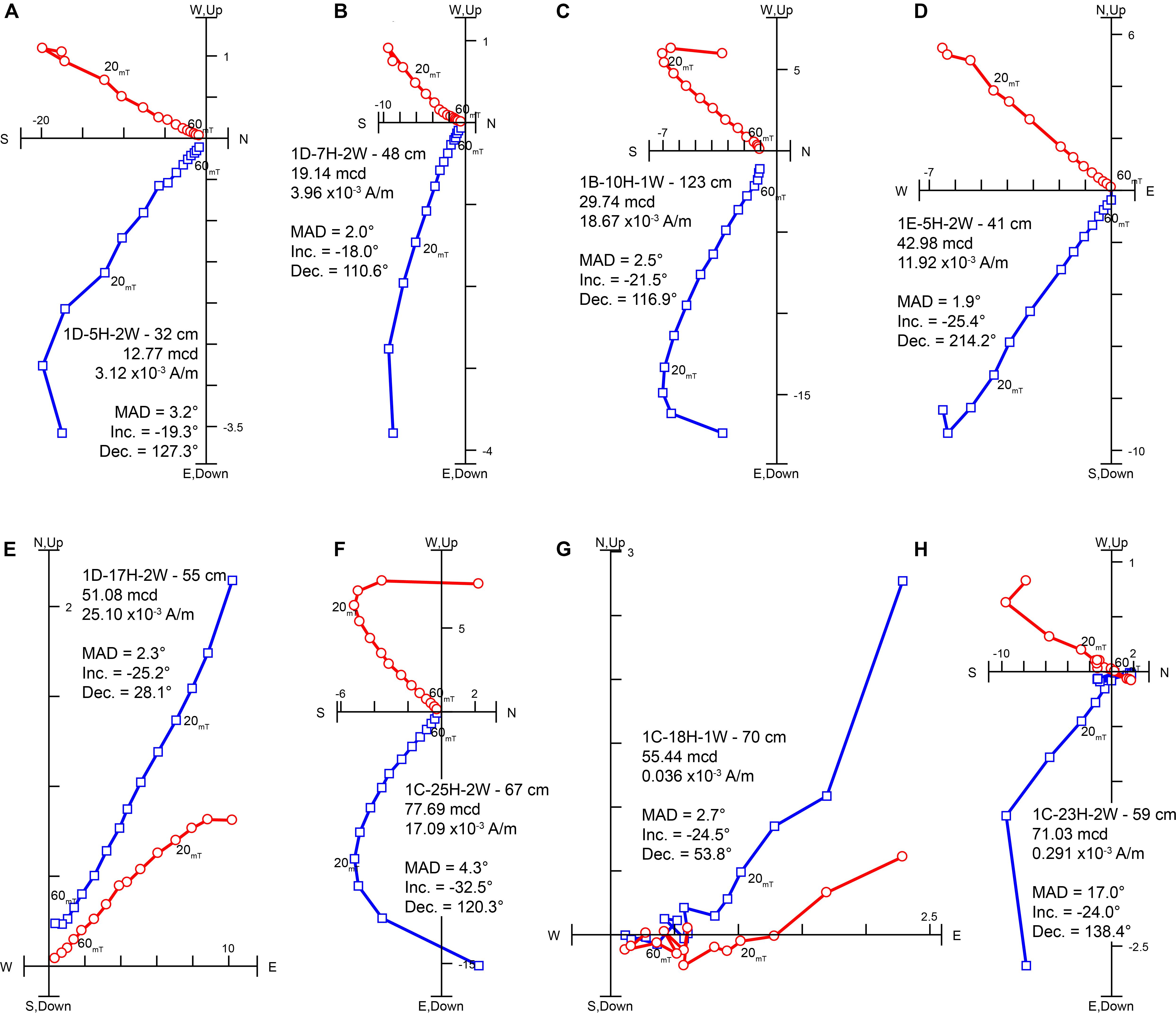
Figure 5. Examples of orthogonal projections of AF demagnetization from u-channel samples. Red data and blue data represent the vertical and horizontal components of the field, respectively. The core section depth, meters composite depth, NRM_{0 mT} intensity value, MAD value, ChRM inclination, and ChRM declination are given. Note the stable and well-defined AF demagnetization structure and relatively low MAD values of samples with NRM_{0 mT} intensity values > 1 × 10^{– 3} A/m (A–F) that contrasts with the more scattered AF demagnetization and higher MAD values of samples with NRM_{0 mT} intensity values < 1 × 10^{– 3} A/m (G,H).

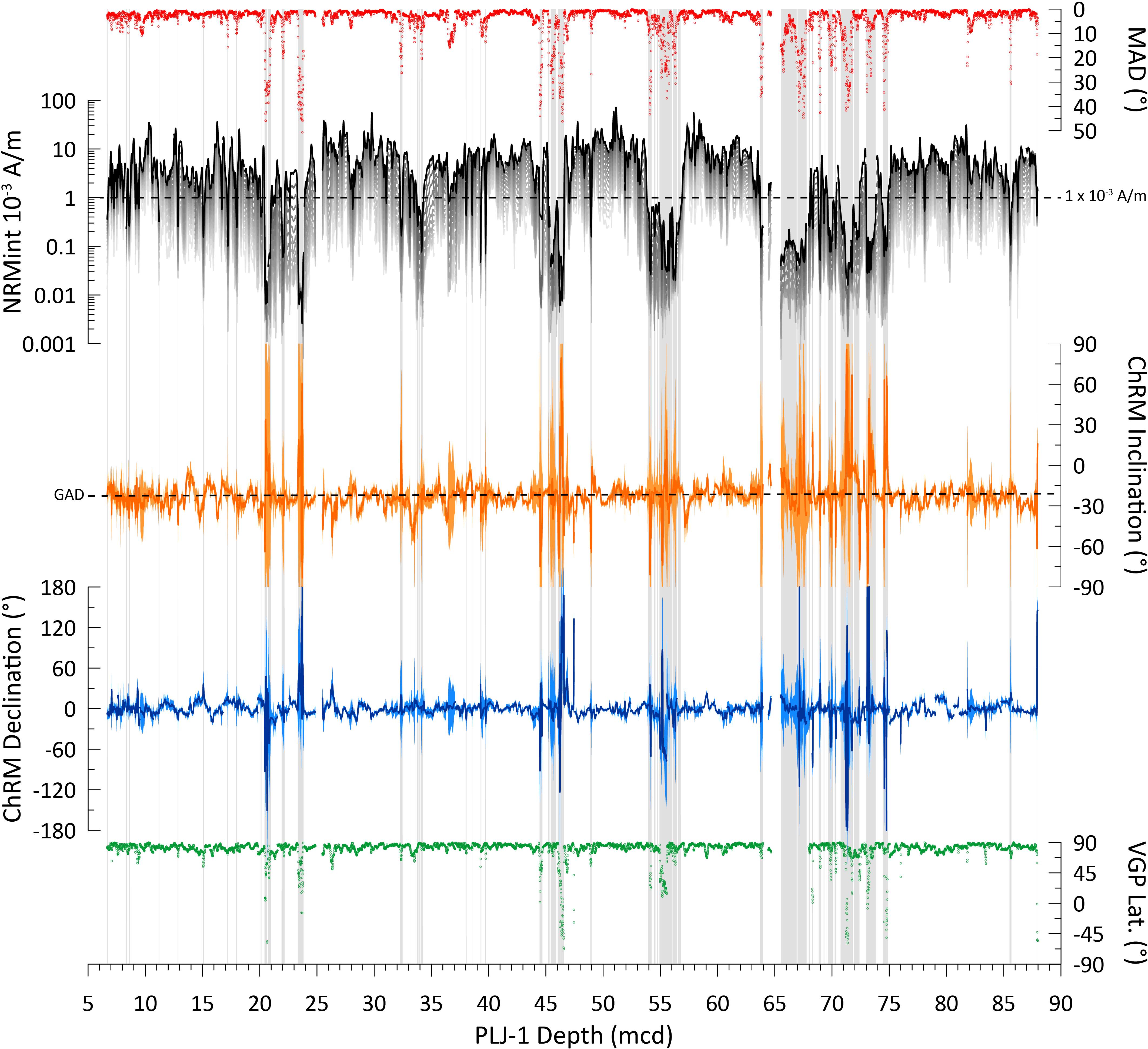
Figure 6. Maximum angular deviation (MAD) values (red points), NRM intensity before (black data) and through progressive AF demagnetization (gray data), component inclination (orange) compared against a predicted value assuming a GAD and corrected (rotated to core mean of zero) component declination (blue), and virtual geomagnetic pole latitude (green points). a95 directional uncertainties (colored shading around the inclination and declination values) are calculated from MAD values using the method of Khokhlov and Hulot (2016). Gray vertical shading denotes NRM_{0 mT} intensity values below a 1 × 10^{– 3} A/m threshold. Note the higher MAD values, greater directional variability, uncertainty, and VGP latitude scatter with lower than threshold NRM_{0 mT} intensity values.

Inclination values of the H-NRMint intervals cluster around the expected value of −21° (median = −23.8°; IQR = −20.1 – −27°) during periods of normal polarity for the site latitude assuming a Geocentric Axial Dipole (GAD) field. VGP latitude of the H-NRMint intervals cluster between +80° and +90° further suggesting that paleomagnetic directions reflect geomagnetic behavior and that the entire record was deposited during the Brunhes chron and is younger than ∼773 ka (Channell et al., 2010; Simon et al., 2019; Singer et al., 2019) (Figure 6), consistent with the U-Th age constraints by Chen et al. (2020). Variability in both inclination and declination of a few tens of degrees throughout the H-NRMint record is consistent with normal secular variation suggesting that the Junín sediments may also preserve non-axial dipole features of the field. During the L-NRMint intervals paleomagnetic directions deviate more widely from expected values (median inclination = −19.47°; IQR = −6.8 – −27.4°), with higher MAD values resulting in greater directional uncertainty. Filtering out the L-NRMint data effectively cleans the lowest quality directional data that are dominantly associated with carbonate rich lithologies, while still retaining 78% of the record. We should note that this threshold filtering process does not discriminate between low NRM intensity data associated with lithologic variations and low intensity data associated with true geomagnetic variability. Therefore, for examination of potential geomagnetic excursion candidates in this, or any other record that follows this approach, the original unfiltered dataset would need to be examined. For Lake Junín, if we exclude the extended L-NRMint interval between 64 and 75 mcd, then eight L-NRMint intervals have VGP latitude values shallower than 45° (Figure 6). However, detailed investigation of each of these intervals revealed that the L-NRMint values resulted from lithogenic and rock magnetic, rather than paleomagnetic, variability and therefore cannot be used as additional chronostratigraphic constraints.

Natural Remanent Magnetization intensity was normalized to generate a proxy for RPI using two methods. First, the NRM intensity following 20 mT AF demagnetization (NRM_{20 mT}) was normalized using MS (NRM_{20 mT}/MS) (Figure 7A). Second, NRM intensity was normalized by ARM intensity over the 20–60 mT AF demagnetization range using the slope method [NRM/ARM_slope)] with the fit of the two datasets monitored using the R-value (Figure 7A). L-NRMint intervals have lower NRM/ARM_slope values (median = 0.09; IQR = 0.06–0.14) and lower average R-values (r = 0.83) than the H-NRMint intervals (median = 0.23; IQR = 0.17 – 0.28; R-value > 0.99). A similar relationship is observed in the NRM_{20 mT}/MS dataset with many of the L-NRMint intervals possessing negative values of NRM_{20 mT}/MS that originate from the weakly negative MS values of the diamagnetic carbonate dominated sediments (Figure 7A). Distributions of normalized ratios reveal the bias that L-NRMint values have for lower ratio values, that lithological variation strongly affects the normalized NRM ratios and the quality of the normalization, and that these poorly defined values can be effectively filtered out by restricting our analysis to the H-NRMint dataset (Figures 7B,C). Neither filtered ratio dataset shows affinity to its normalizer suggesting little to no magnetic concentration influence on the H-NRMint normalized ratios (Figures 7D,E). Long period changes in the H-NRMint NRM/ARM_slope and H-NRMint NRM_{20 mT}/MS values largely track each other suggesting a common driver of variability, however, the NRM_{20 mT}/MS data appears more afflicted by higher frequency spike noise and negative values (Figure 7A). This increased variability likely relates to discrete intervals of lithologic variability that are likely inefficiently normalized using MS compared to ARM and NRM that are only sensitive to remanence carrying minerals and to the different response functions of the measurements. As a result we restrict the following discussion to the H-NRMint NRM/ARM_slope dataset, which coupled with R-values > 0.99, implies a well-defined and stable ratio.

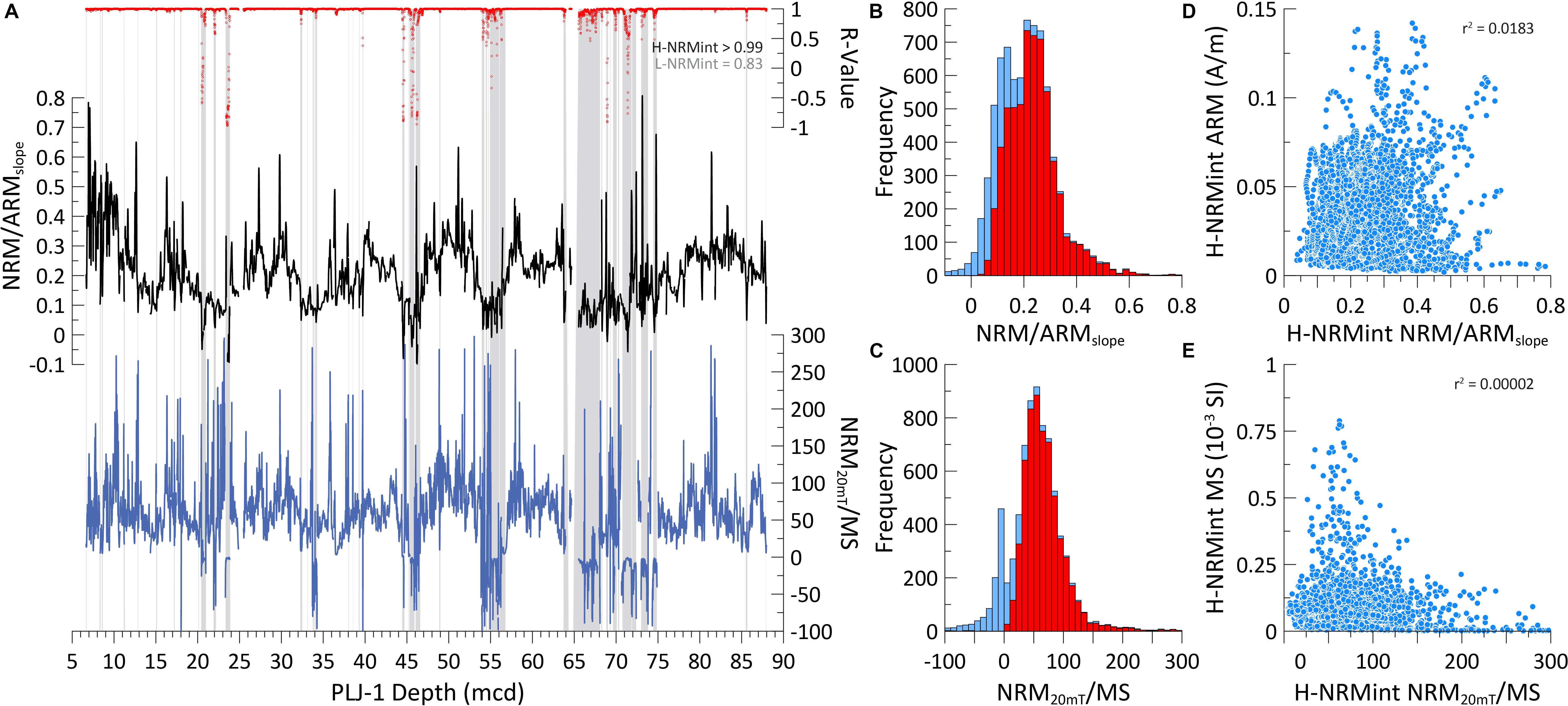
Figure 7. (A) Normalized remanence ratios NRM_{20 mT}/MS (blue) and NRM/ARM_slope (black) values and the associated R-value (red). Gray vertical shading highlights NRM_{0 mT} intensity values below a threshold of 1 × 10^{– 3} A/m as in Figure 6. Median R-values of data with NRM intensity higher than the threshold (H-NRMint) exceed 0.99 while R-values of data with NRM intensity lower than the threshold (L-NRMint) are much lower; median values of these two populations are annotated. (B) Distribution of all NRM/ARM_slope data (blue) and the H-NRMint NRM/ARM_slope data (red). (C) Distribution of all NRM_{20 mT}/MS data (blue) and the H-NRMint NRM_{20 mT}/MS data (red). Note the L-NRMint data are biased toward lower, and in the case of NRM_{20 mT}/MS negative, values. (D) NRM/ARM_slope values plotted against ARM intensity values for the H-NRMint dataset. (E) NRM_{20 mT}/MS values plotted against MS values for the H-NRMint dataset. Note the lack of correlation between the normalized ratio and its normalizer for the H-NRMint datasets suggesting little influence of bulk magnetic concentration parameters on the normalized ratios.

Together, the demagnetization behavior, coherent directions, and well-defined and behaved normalized remanence ratios yield attributes that often result in the generation of reliable paleomagnetic records. Tauxe (1993) proposed a set of criteria to evaluate the reliability of sediment paleomagnetic and paleointensity records which we briefly summarize here: (1) the NRM must be carried by stable magnetite with a single well-defined component to the magnetization; (2) the detrital remanence must exhibit no inclination error; (3) concentration variations of more than about an order of magnitude should be avoided; (4) normalization by multiple methods should yield consistent results; (5) normalized intensity records should not be coherent with bulk rock magnetic parameters and; (6) records from a given region should agree within limits of a common timescale. Rock magnetic and paleomagnetic properties showed that samples are dominated by ferrimagnetic mineralogies (e.g., magnetite, titanomagnetite, and/or maghemite), and that by filtering the L-NRMint values from the dataset preferentially removes intervals dominated by non-ferrimagnetic components (Figures 2–4). In turn, this retains the most well-defined single-component ChRM’s (Figure 5), reduces median MAD values to 1.7° and removes the more highly scattered directional variability (Figure 6), reduces the variance in MS and ARM values (90% of H-NRMint ARM intensity values are within one order of magnitude) (Figure 2), and results in normalized ratios that have little to no dependence on their normalizer (Figure 7D). As a result the H-NRMint dataset predominantly satisfies the first five criteria of Tauxe (1993) suggesting that the NRM/ARM_slope record is likely capable of recording and preserving variability in geomagnetic field intensity.

To determine if Lake Junín sediments preserve a record of geomagnetic field intensity changes, we would expect it to reproduce the variability in independently dated reference records (Tauxe, 1993; Stoner and St-Onge, 2007). The H-NRMint filtered NRM/ARM_slope record is shown on the Chen et al. (2020) age model alongside the PISO-1500 global relative paleointensity stack (Channell et al., 2009) and the PADM-2M (Ziegler et al., 2011) axial dipole moment model in Figure 8. Similar features are identifiable and appear to be correlatable across the records (Figure 8). Low NRM/ARM_slope values appear associated with the low geomagnetic intensity values associated with the Laschamp excursion (∼41 ka), but between ∼60 and ∼110 ka on the Chen et al. (2020) age model NRM/ARM_slope values are relatively low and invariant making it difficult to correlate to PISO-1500 or PADM-2M. This carbonate dominated interval (lithotype 1) between 20–24 mcd has some of the weakest H-NRMint values (Figure 2), possibly explaining the reduced quality of this interval. As the upper ∼50 ka is well constrained by radiocarbon and two U-Th age constraints exist around ∼70 ka we focus our paleomagnetic investigations on the record prior to 120 ka.

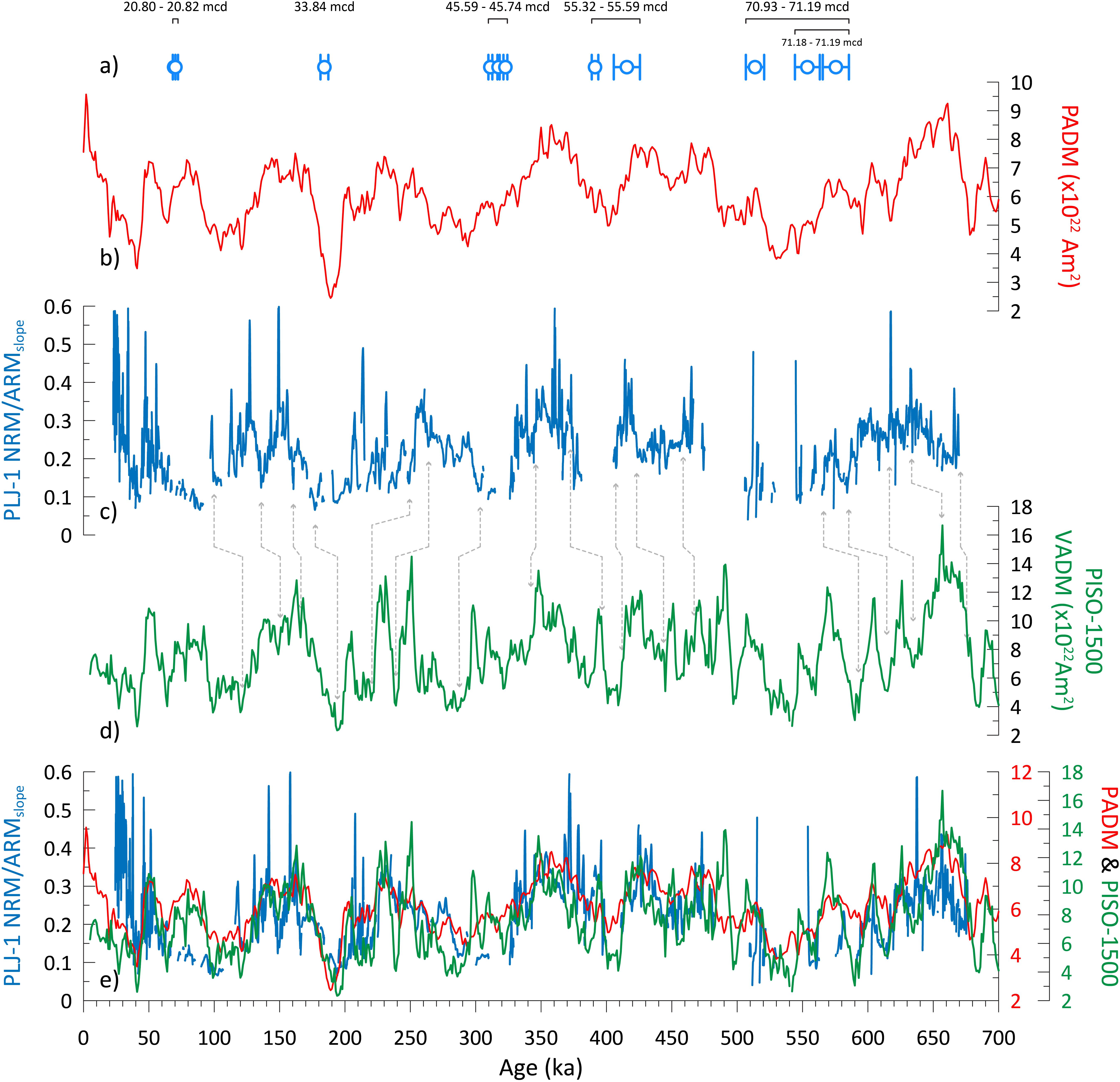
Figure 8. (a) The 12 U-Th age constraints and 1-sigma uncertainty from the five horizons used to construct the age-depth model of Chen et al. (2020); the depth ranges of the dated samples are also given. (b) PADM-2M (red) dipole moment model of Ziegler et al. (2011). (c) The filtered Lake Junín H-NRMint NRM/ARM_slope RPI estimate (blue) using the age model of Chen et al. (2020). (d) PISO-1500 (green) RPI stack of Channell et al. (2009). Gray dashed lines between the Junín record and the PISO-1500 RPI stack is used to improve the correlation between the two from r = 0.15 to r = 0.51. (e) Comparison of PADM-2M, PISO-1500, and Junín RPI estimate after age adjustment using the gray tie-points. Correlation is restricted to the period prior to 120 ka (see text for further details).

In detail, the similarity of the three records varies through time with variability in the Lake Junín NRM/ARM_slope record appearing to both lead and lag changes in the global intensity estimate reference records. Although magnetic acquisition may play a role, any lock-in depth effect would only be expected to cause hundreds to a few thousand years of delay given sedimentation rates in excess of 10 cm/kyr (Roberts and Winklhofer, 2004; Suganuma et al., 2011). Instead, it is more likely that these longer-period offsets result from variations in sedimentation rate linked to changes in the regional environment, including lake level and glacial extent. Clearly sediment lithology is not adequately captured in the underconstrained radiometric-based age-model. By adopting 17 tie points (Table 1) based on the visual correlations in Figure 8 the correlation coefficient (r) between the NRM/ARM_slope record from Lake Junín and PISO-1500 improves from 0.15 to 0.51 and 0.62 to PADM-2M (Figure 8e), approaching the r = 0.69 correlation between PISO-1500 and PADM-2M over the same time period. The improved correlation argues for viability of a paleointensity assisted chronology for the Lake Junín record.

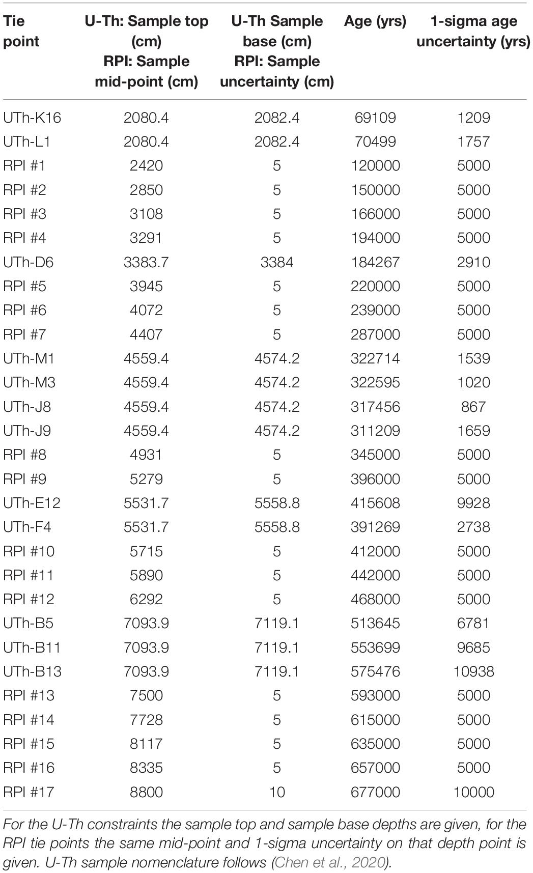
Table 1. Tie points, sample depths, age, and age uncertainty for the U-Th and RPI age-depth constraints used for the Undatable Lake Junín age model.

Discussion

Normalized remanence ratios such as NRM/ARM_slope are frequently generated to address two main questions: (1) to provide an estimation of geomagnetic relative paleointensity (RPI) that can be used to comment on some behavioral aspect of the geodynamo (e.g., reversals, excursions, and/or non-dipolar PSV behavior) (Stoner et al., 2002, 2013; Valet et al., 2005; Channell et al., 2009; Channell, 2017); and/or (2) to provide a continuous record of paleomagnetic field intensity variability that can be compared to well-dated stacks for the purpose of chronostratigraphy (Evans et al., 2007; Hatfield et al., 2016; Blake-Mizen et al., 2019; Channell et al., 2019). Although the differences between these two aims may seem subtle, the distinction can be important. RPI records used to define and study some aspect of the geodynamo should be of the utmost quality, ideally homogenous in composition, and be unambiguously clean of environmental influences or geochemical effects (Stoner and St-Onge, 2007). Natural variations in lithology can often complicate remanence normalization, but if these effects are not too severe, then RPI proxies (i.e., NRM/ARM_slope) can be adequately matched to RPI reference templates to provide chronological control (Stoner et al., 2000, 2003; Evans et al., 2007; Blake-Mizen et al., 2019; Channell et al., 2019). By these criteria, the sedimentological and rock magnetic variability outlined in Figures 2–4 precludes the use of the Lake Junín record for detailed study of geomagnetic variability. However, the filtering process outlined in Figure 7 to retain the highest quality data and the improved RPI correlations outlined in Figure 8 suggest that we can potentially use the NRM/ARM_slope values of the Lake Junín sediments to provide additional age model constraints to refine the existing chronology.

Age Model Construction

To integrate the paleomagnetic data with the existing age-depth points we use the MatLab-based age-depth modeling program Undatable (Lougheed and Obrochta, 2019). The advantage of using Undatable over other available age-depth modeling programs is that it allows for uncertainties in both age and depth, for a series of different types of age control points to be incorporated (e.g., absolute ages and tie-points), and for selective bootstrapping of the included ages (Lougheed and Obrochta, 2019). The age-depth tie points we use take three forms: (1) the 79 radiocarbon dates for the upper 17 mcd (Woods et al., 2019); (2) the 12 U-Th ages grouped around the 5 interglacial horizons (Chen et al., 2020); and (3) the 17 tie points made between the Junín NRM/ARM_slope record and PISO-1500 (Figure 8). The 29 combined U-Th and RPI tie points are listed in Table 1. For the radiocarbon dates, we assumed uniform depth uncertainty based on the sampling interval (often 2 cm). When running Undatable, radiocarbon calibration to calendar years using IntCal13 (Reimer et al., 2013) is automatically performed with MatCal (Lougheed and Obrochta, 2016), which uses highest posterior density to calculate the discrete one- and two-sigma ranges. Where U-Th age constraints occur within a few tens of centimeters of each other, we group the dated horizons within a uniform depth window using the maximum range for the grouped samples. This approach is used for the two U-Th age constraints at 20.80 and 20.82 mcd, the four constraints between 45.59 and 45.74 mcd, the two constraints at 55.32 and 55.58 mcd, and the three deepest constraints between 70.94 and 71.19 mcd (see Figure 8). By grouping the age constraints in this manner we combine their age probability density functions (PDFs) in Undatable and sample the entire interval using the information from the cumulative, multi-modal pdf’s over the grouped depth range [see Fujiwara et al. (2019) for an explanation and practical example]. Age uncertainties for the individual U-Th age constraints uses the 1-sigma age uncertainty reported by Chen et al. (2020) (Table 1). For the paleomagnetic tie points, we used a Gaussian depth uncertainty (in most cases the range used was ±5 cm) which is more appropriate than uniform uncertainty when aligning reference series using tie points in Undatable (Lougheed and Obrochta, 2019). We adopt a conservative 1-sigma age uncertainty of ±5,000 years for the majority of paleomagnetic tie-points to account for “fuzziness” in paleomagnetic acquisition processes between records (e.g., sediment lock-in), potential aliasing of the paleomagnetic signal, and age model differences in different reference curves; e.g., the age of the RPI-low associated with the Iceland basin excursion varies between PISO-1500 (194 ka), SINT-2000 (190 ka), HINAPIS (187.5 ka), and PADM-2M (189 ka) (Valet et al., 2005; Channell et al., 2009; Ziegler et al., 2011; Xuan et al., 2016). The tie-point uncertainties are much greater than the depth uncertainties, but are similar in duration to the 1-sigma uncertainties reported for the U-Th age constraints by Chen et al. (2020) and are of the same order of magnitude as age-model uncertainties for the same features in different RPI stacks. The lowermost age-depth constraint provides an end point for the age-depth simulation in Undatable, cannot be included in the bootstrapping routine, and therefore has greater weight in the resulting age model (Lougheed and Obrochta, 2019). As a result we adopt a larger depth uncertainty of ±10 cm and a 1-sigma age uncertainty of 10,000 years for the basal paleomagnetic tie point, to provide a less rigid constraint to facilitate more reliable uncertainty estimates.

Undatable was run using 100,000 simulations, an xfactor of 0.1, and a bootpc of 30. The xfactor controls the sediment accumulation rate assumptions between pairs of age-depth constraints with larger values leading to greater freedom and therefore greater “uncertainty bubbles” (Lougheed and Obrochta, 2019). Published age models using Undatable have typically adopted an xfactor value of 0.1 (Lougheed and Obrochta, 2019). Bootpc controls the percentage of age-depth constraints that are bootstrapped (i.e., randomly removed) during each simulation, with a higher bootpc value allowing the age-model to explore a larger number of routing possibilities that produces a smoother result with larger uncertainty (Lougheed and Obrochta, 2019). As the radiocarbon interval is well-defined (Woods et al., 2019) and the major focus of the age-model refinement is the period >120 ka we only bootstrap the U-Th and paleomagnetic tie-points to prevent their under-sampling in the bootstrapping routine if all available dates had been used. Experiments were run varying the xfactor (0.05, 0.1, and 0.2) and bootpc (10, 20, 30, 40, and 50%) values, but these had little impact on the mean age model which remained entirely within the 1-sigma error of the results of the xfactor = 0.1, bootpc = 30 derived age-depth model.

The resulting age-depth plot is shown in Figure 9B alongside the existing radiometric-only Bacon (Blaauw and Christen, 2011) derived age model of Chen et al. (2020) that was parameterized using; thickness = 50 cm, acc.mean = 80 yr/cm, acc.shape = 2.0, mem.strength = 15, and mem.mean = 0.8 (Figure 9A). In general terms the two age models possess a similar basal age, occurring during MIS 16, similar average sedimentation rates around 11 cm/kyr, and similar average uncertainties at the 95% confidence interval for sediments older then ∼120 ka; ∼39 ka for the U-Th based age model, ∼37 ka for the new integrated age model. However, the greater density of age-depth constraints prior to ∼120 ka in the new age model results in clear variations in sedimentation rate, age model structure, and age model uncertainty in Figure 9C.

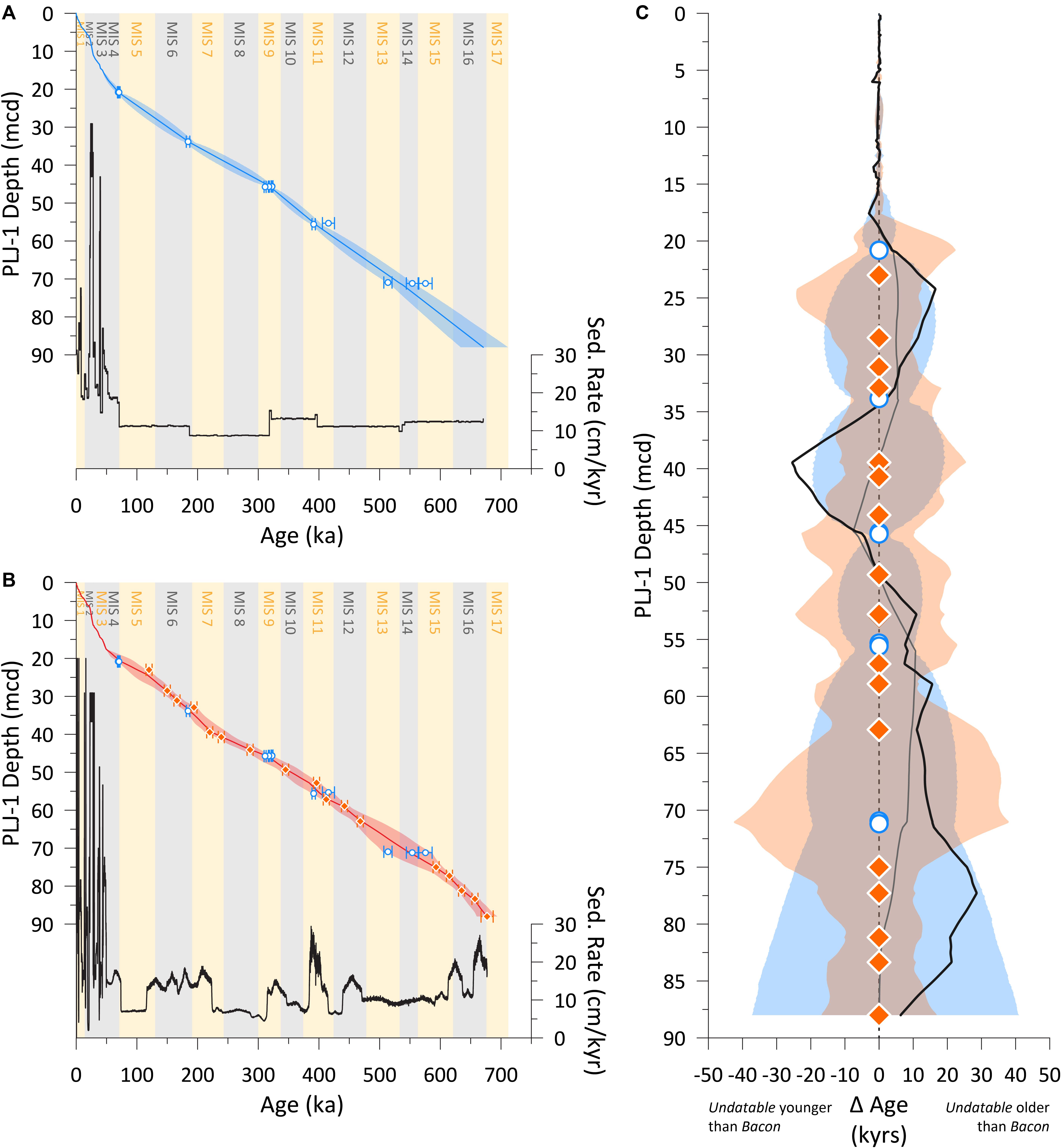
Figure 9. (A) The existing Bacon age model (blue line) of Chen et al. (2020) reproduced from Figure 1 for comparison. (B) The new Undatable derived age-depth model (red line) using 79 radiocarbon dates (not shown for clarity) from Woods et al. (2019), 18 U-Th age constraints for the Lake Junín splice [blue symbols as in A; (Chen et al., 2020)], and 17 paleomagnetic tie points (orange symbols) identified in Figure 8. The 2-sigma uncertainty (red shading) and calculated mean sedimentation rate (black line) is also shown. Marine Isotope Stages (MIS) are denoted by gray shading for glaciations and yellow shading interglaciations as defined in LR04 (Lisiecki and Raymo, 2005). (C) The Bacon age-depth mean-age model is subtracted from the Undatable age-depth mean-age model (black line) and the radiometric only Undatable age-depth mean-age model (thinner gray line, see text for details). Positive [negative] values imply an older [younger] age of the Undatable age-depth models compared to the Bacon age-depth model. The depth of U-Th age constraints (open blue circles) and paleomagnetic tie-points (orange diamonds) are shown alongside the uncertainty envelope of the existing Bacon age-depth model (blue) and new Undatable age-depth model (orange). Note that the offset of the two age models mostly falls within the uncertainty envelope of both age models.

In order to examine whether these differences result from the inclusion of the paleomagnetic data, or the use of different age-depth modeling software, we reran Undatable using only the radiometric-based ¹⁴C and U-Th ages. We adopted the same xfactor and bootpc parameters as before and constrained the basal age at 670.7 ka as projected by the mean Bacon age model. The differences between the Undatable and the Bacon radiometric-only results are shown as the thinner gray line in Figure 9C. In the interval 0–50 mcd, the average difference between the Bacon and Undatable mean results is 2.8 kyrs (maximum = 7.6 kyrs) (Figure 9C). These differences are an order of magnitude lower than the uncertainty structures of both age-models and imply relatively little difference between the two age-depth modeling approaches through these intervals. Between ∼50 and ∼88 mcd the radiometric-only Undatable age-model is generally older than the Bacon derived radiometric-only age-model with a maximum age-difference averaging around 10 kyrs between 55 and 71 mcd (Figure 9C). These differences likely arise from the way that the closely grouped data are input into Bacon and Undatable, respectively. While the Undatable age model is effectively sampling a cumulative and multi-modal PDF of the combined ages within a grouped interval, Bacon treats the individual ages as a spread of separate data points. For the U-Th age constraints clustered around 55 and 71 mcd the youngest age in each case has a lower uncertainty than the older ages from the same grouping (Figure 8). As the Bacon algorithm rewards samples with lower uncertainty (Blaauw and Christen, 2011), these younger ages are favored over the older and more uncertain ages in the close grouping. Indeed, the U-Th age constraints at 415.6 and 575.5 ka are effectively ignored by the Bacon algorithm, falling entirely outside the 2-sigma uncertainty structure of the resulting age model (Figure 9A). As a result the Bacon derived age-model is 9.7 and 8.2 kyrs younger than the Undatable age model at ∼55.5 and ∼71 mcd (the depths of the U-Th constraints) respectively (Figure 9C).

While the age-depth modeling approach used can account for a large part of the age-model difference between 55 and 71 mcd, significant deviations of the black and gray lines in Figure 9C reveals that the inclusion of paleomagnetic tie points also drives age-model variations. These deviations are greatest at ∼24.5, ∼40, and ∼77.5 mcd (Figure 9C). Between ∼34 and ∼50 mcd the Undatable age model is younger than the Bacon derived U-Th age model, while between ∼21 and ∼34 mcd and ∼50 and ∼88 mcd the Undatable age model is older than the Bacon age model. In general the uncertainty of the Undatable age model is greater than that of the Bacon age model, particularly around the deeper U-Th dated horizons (Figure 9C). We argue that this greater uncertainty and conservative approach is likely more appropriate as Chen et al. (2020) found no reason to reject the 415.6 and 575.5 ka U-Th ages that appear largely ignored by the Bacon age model. However, while the greater variability in age, sedimentation rate, and uncertainty structure in the Undatable age-model results from the inclusion of the paleomagnetic tie points, almost all of this age-model variability falls within the 2-sigma uncertainty of the original Bacon age model (Figure 9C).

Within the resolution of the Undatable age model (∼10⁴ yrs; Figure 9B), sedimentation rate changes appear to mostly coincide with glacial-interglacial cycles. For example, sedimentation rates appear to be higher during the four periods of largest Pleistocene global ice volume associated with MIS 16, MIS 12, MIS 6, and MIS 2. These intervals are also characterized by higher magnetic concentration and MDF_ARM values suggesting that increases in clastic flux that occurred during the last local glacial maximum (Woods et al., 2019) may be a consistent and reproducible feature of the Lake Junín record over multiple glacial cycles. In addition to increases in glacial sediment fluxes, increased sedimentation rates also appear associated with the MIS 11 and MIS 9 interglaciations and the peak interglacial substages of MIS 5e and MIS 7c-a Figure 9B. These increases suggest that in addition to increases in glacial-clastic flux, variations in the efficiency of the in-lake carbonate pump affects sediment accumulation rate within the lake Junín basin as observed in the Holocene (Woods et al., 2019). These variations were not able to be resolved by the radiometric-based Bacon age model. Thus, the addition of the paleomagnetic chronological constraints to the existing radiometric derived age-model improves the chronological framework for Lake Junín, and establishes an age model capable of addressing the larger goals of the Lake Junín project.

Conclusion

The time interval covered and varying lithology of the Lake Junín sediments dictate that no single chronometer is able to develop a chronology required to address the larger goals of the Lake Junín project. Only the upper ∼17 mcd are within the radiocarbon window and the older U-Th dated intervals are limited to authigenic carbonate-rich horizons that are largely deposited during interglaciations. As a result, beyond MIS 3, glacial-interglacial variations in sedimentation rate remained unconstrained. Paleomagnetic data acquired from the Lake Junín splice record are of variable quality. Higher lithogenic content associated with glacial advances results in higher quality paleomagnetic records capable of constraining sedimentation rates, whereas carbonate facies are generally poorer paleomagnetic recorders. Filtering of the paleomagnetic record based upon magnetic concentration effectively separated these components, while still preserving almost 80% of the normalized remanence record that pass criteria for relative paleointensity estimates. Comparison to global intensity estimate reference curves show significant similarities on independent timescales with correlations greatly improved through minor age adjustments within the uncertainties of U-Th chronology. These age adjustments during glacial periods that were previously unconstrained by U-Th dating provide a series of new tie-points that were integrated with the radiometric data in the age-depth modeling program Undatable to generate a new age-depth model for the Lake Junín splice and provide an estimate of uncertainty. The new age-depth model remains within the 2-sigma uncertainty structure of the existing radiometric-based age-model, but now produces glacial-interglacial variation in sedimentation rate that are similar to those found in the radiocarbon dated interval. By integrating the different chronometers, each with optimal temporal windows and/or lithologies of operation an improved orbital scale age model could be developed with realistic and transparent uncertainties that can facilitate the larger goals of the Lake Junín project.

Data Availability Statement

All datasets generated for this study are included in the article/Supplementary Material.

Author Contributions

JS, MA, DR, and DM conceived the Lake Junín project and acquired funding. RH and JS designed the paleomagnetic study of which this manuscript is the focus. RH, KS, and AM measured samples. RH and JS interpreted the data. All authors contributed to the writing, revision, and/or editing of the manuscript.

Funding

This research was carried out with support from the United States National Science Foundation awards EAR-1400903 (Stoner), EAR-1404113 (Abbott), EAR-1404414 (McGee), and EAR-1402076 (Rodbell) and from support by the ICDP, which in the United States is operated out of the Continental Scientific Drilling Coordination Office (CSDCO) at the University of Minnesota.

Conflict of Interest

The authors declare that the research was conducted in the absence of any commercial or financial relationships that could be construed as a potential conflict of interest.

Acknowledgments

The Lake Junín Project would not have been possible without the team of drillers from DOSECC Exploration Services (United States), GEOTEC (Peru), and the expertise of Doug Schnurrenberger, Kristina Brady Shannon, and Mark Shapley of CSDCO. Logistical assistance in the field was provided by Bryan Valencia, Angela Rozas-Davila, James Bartle, and Cecilia Oballe. RH would like to thank Cristina García-Lasanta and Bernie Housen at WWU for help measuring samples and Stephen Obrochta at Akita University for comments on using Undatable. We thank the three reviewers whose detailed and thoughtful comments improved this manuscript.

Supplementary Material

The Supplementary Material for this article can be found online at: https://www.frontiersin.org/articles/10.3389/feart.2020.00147/full#supplementary-material

DATA SHEET S1 | U-channel and color profile data on depth and age. Hysteresis and ARM ratio parameters on depth and age. HTMS data on heating (red) from 25-700 degrees Celsius and cooling (blue) from 700–50 degrees Celsius interpolated to the nearest degree.

References

Banerjee, S. K., King, J., and Marvin, J. (1981). A rapid method for magnetic granulometry with applications to environmental studies. Geophys. Res. Lett. 8, 333–336. doi: 10.1029/GL008i004p00333
Blaauw, M., and Christen, J. A. (2011). Flexible paleoclimate age-depth models using an autoregressive gamma process. Bayesian Anal. 6, 457–474. doi: 10.1214/11-BA618
Blake-Mizen, K., Hatfield, R. G., Stoner, J. S., Carlson, A. E., Xuan, C., Walczak, M., et al. (2019). Southern Greenland glaciation and Western Boundary Undercurrent evolution recorded on Eirik Drift during the late Pliocene intensification of Northern Hemisphere glaciation. Quat. Sci. Rev. 209, 40–51. doi: 10.1016/j.quascirev.2019.01.015
Burns, S. J., Welsh, L. K., Scroxton, N., Cheng, H., and Edwards, R. L. (2019). Millennial and orbital scale variability of the South American Monsoon during the penultimate glacial period. Sci. Rep. 9, 1–5. doi: 10.1038/s41598-018-37854-3
Chang, L., Roberts, A. P., Tang, Y., Rainford, B. D., Muxworthy, A. R., and Chen, Q. (2008). Fundamental magnetic parameters from pure synthetic greigite (Fe3S4). J. Geophys. Res. Solid Earth 113:B06104. doi: 10.1029/2007JB005502
Chang, L., Vasiliev, I., Van Baak, C., Krijgsman, W., Dekkers, M. J., Roberts, A. P., et al. (2014). Identification and environmental interpretation of diagenetic and biogenic greigite in sediments: a lesson from the Messinian Black Sea. Geochem. Geophys. Geosyst. 15, 3612–3627. doi: 10.1002/2014GC005411
Channell, J. E. T. (2017). Mid-Brunhes magnetic excursions in marine isotope stages 9, 13, 14, and 15 (286, 495, 540, and 590 ka) at North Atlantic IODP Sites U1302/3, U1305, and U1306. Geochem. Geophys. Geosyst. 18, 473–487. doi: 10.1002/2016GC006626
Channell, J. E. T., Hodell, D. A., Singer, B. S., and Xuan, C. (2010). Reconciling astrochronological and 40Ar/39Ar ages for the Matuyama-Brunhes boundary and late Matuyama Chron. Geochem. Geophys. Geosyst. 11:Q0AA12. doi: 10.1029/2010GC003203
Channell, J. E. T., Hodell, D. A., Xuan, C., Mazaud, A., and Stoner, J. S. (2008). Age calibrated relative paleointensity for the last 1.5 Myr at IODP Site U1308 (North Atlantic). Earth Planet. Sci. Lett. 274, 59–71. doi: 10.1016/j.epsl.2008.07.005
Channell, J. E. T., Mazaud, A., Sullivan, P., Turner, S., and Raymo, M. E. (2002). Geomagnetic excursions and paleointensities in the Matuyama Chron at Ocean Drilling Program Sites 983 and 984 (Iceland Basin). J. Geophys. Res 107, EM1–EM14. doi: 10.1029/2001jb000491
Channell, J. E. T., Wright, J. D., Mazaud, A., and Stoner, J. S. (2014). Age through tandem correlation of Quaternary relative paleointensity (RPI) and oxygen isotope data at IODP Site U1306 (Eirik Drift. SW Greenland). Quat. Sci. Rev. 88, 135–146. doi: 10.1016/j.quascirev.2014.01.022
Channell, J. E. T., Xuan, C., and Hodell, D. A. (2009). Stacking paleointensity and oxygen isotope data for the last 1.5 Myr (PISO-1500). Earth Planet. Sci. Lett. 283, 14–23. doi: 10.1016/j.epsl.2009.03.012
Channell, J. E. T., Xuan, C., Hodell, D. A., Crowhurst, S. J., and Larter, R. D. (2019). Relative paleointensity (RPI) and age control in Quaternary sediment drifts off the Antarctic Peninsula. Quat. Sci. Rev. 211, 17–33. doi: 10.1016/j.quascirev.2019.03.006
Chen, C. Y., McGee, D., Woods, A., Pérez, L., Hatfield, R. G., Edwards, R. L., et al. (2020). U-Th Dating of Lake Sediments: Lessons From the 700 kyr Sediment Record of Lake Junín, Peru. Available online at: https://doi.org/10.31223/osf.io/c765k (accessed May 4, 2020).
Dankers, P. (1981). Relationship between median destructive field and remanent coercive forces for dispersed natural magnetite, titanomagnetite and hematite. Geophys. J. R. Astron. Soc. 64, 447–461. doi: 10.1111/j.1365-246X.1981.tb02676.x
Day, R., Fuller, M., and Schmidt, V. A. (1977). Hysteresis properties of titanomagnetites: grain-size and compositional dependence. Phys. Earth Planet. Inter. 13, 260–267. doi: 10.1016/0031-9201(77)90108-X
Dekkers, M. J. (1989). Magnetic properties of natural pyrrhotite. II. High- and low-temperature behaviour of Jrs and TRM as function of grain size. Phys. Earth Planet. Inter. 57, 266–283. doi: 10.1016/0031-9201(89)90116-7
Dekkers, M. J., Passier, H. F., and Schoonen, M. A. A. (2000). Magnetic properties of hydrothermally synthesized greigite (Fe3S4)-II. High- and low-temperature characteristics. Geophys. J. Int. 141, 809–819. doi: 10.1046/j.1365-246X.2000.00129.x
Edwards, R. L., Gallup, C. D., and Cheng, H. (2003). Uranium-series dating of marine and lacustrine carbonates. Rev. Mineral. Geochem. 52, 363–405. doi: 10.2113/0520363
Evans, H. F., Channell, J. E. T., Stoner, J. S., Hillaire-Marcel, C., Wright, J. D., Neitzke, L. C., et al. (2007). Paleointensity-assisted chronostratigraphy of detrital layers on the Eirik Drift (North Atlantic) since marine isotope stage 11. Geochem. Geophys. Geosyst. 8, 1–23. doi: 10.1029/2007GC001720
Fritz, S. C., Baker, P. A., Seltzer, G. O., Ballantyne, A., Tapia, P., Cheng, H., et al. (2007). Quaternary glaciation and hydrologic variation in the South American tropics as reconstructed from the Lake Titicaca drilling project. Quat. Res. 68, 410–420. doi: 10.1016/j.yqres.2007.07.008
Fujiwara, O., Aoshima, A., Irizuki, T., Ono, E., Obrochta, S. P., Sampei, Y., et al. (2019). Tsunami deposits refine great earthquake rupture extent and recurrence over the past 1300 years along the Nankai and Tokai fault segments of the Nankai Trough, Japan. Quat. Sci. Rev 227:105999. doi: 10.1016/J.QUASCIREV.2019.105999
Hatfield, R. G., Reyes, A. V., Stoner, J. S., Carlson, A. E., Beard, B. L., Winsor, K., et al. (2016). Interglacial responses of the southern Greenland ice sheet over the last 430,000 years determined using particle-size specific magnetic and isotopic tracers. Earth Planet. Sci. Lett. 454, 225–236. doi: 10.1016/j.epsl.2016.09.014
Hatfield, R. G., Woods, A., Lehmann, S. B., Weidhaas, N. IV, Chen, C. Y., Abbott, M. B., et al. (2020). Stratigraphic correlation and splice generation for sediments recovered from a large lake drilling project: an example from Lake Junín, Peru. J. Paleolimnol. 63, 83–100. doi: 10.1007/s10933-019-00098-w
Johnson, H. P., Lowrie, W., and Kent, D. V. (1975). Stability of anhysteretic remanent magnetization in fine and coarse magnetite and maghemite particles. Geophys. J. R. Astron. Soc. 41, 1–10. doi: 10.1111/j.1365-246X.1975.tb05480.x
Kanner, L. C., Burns, S. J., Cheng, H., and Edwards, R. L. (2012). High-latitude forcing of the South American summer monsoon during the last glacial. Science 335, 570–573. doi: 10.1126/science.1213397
Khokhlov, A., and Hulot, G. (2016). Principal component analysis of palaeomagnetic directions: converting a maximum angular deviation (MAD) into an α95angle. Geophys. J. Int. 204, 274–291. doi: 10.1093/gji/ggv451
King, J., Banerjee, S. K., Marvin, J., and Özdemir, Ö (1982). A comparison of different magnetic methods for determining the relative grain size of magnetite in natural materials: some results from lake sediments. Earth Planet. Sci. Lett. 59, 404–419. doi: 10.1016/0012-821X(82)90142-X
King, J. W., Banerjee, S. K., and Marvin, J. (1983). A new rock-magnetic approach to selecting sediments for geomagnetic paleointensity studies: application to paleointensity for the last 4000 years. J. Geophys. Res. 88, 5911–5921. doi: 10.1029/JB088iB07p05911
Kirschvink, J. L. (1980). The least−squares line and plane and the analysis of palaeomagnetic data. Geophys. J. R. Astron. Soc. 62, 699–718. doi: 10.1111/j.1365-246X.1980.tb02601.x
Lisiecki, L. E., and Raymo, M. E. (2005). A pliocene-pleistocene stack of 57 globally distributed benthic δ 18O records. Paleoceanography 20, 1–17. doi: 10.1029/2004PA001071
Liu, J. (2004). High-resolution analysis of early diagenetic effects on magnetic minerals in post-middle-Holocene continental shelf sediments from the Korea Strait. J. Geophys. Res. 109:15. doi: 10.1029/2003JB002813
Lougheed, B. C., and Obrochta, S. P. (2016). MatCal: open source bayesian 14C age calibration in Matlab. J. Open Res. Softw. 4:e42. doi: 10.5334/jors.130
Lougheed, B. C., and Obrochta, S. P. (2019). A rapid, deterministic age-depth modeling routine for geological sequences with inherent depth uncertainty. Paleoceanogr. Paleoclimatol. 34, 122–133. doi: 10.1029/2018PA003457
Lougheed, B. C., Snowball, I., Moros, M., Kabel, K., Muscheler, R., Virtasalo, J. J., et al. (2012). Using an independent geochronology based on palaeomagnetic secular variation (PSV) and atmospheric Pb deposition to date Baltic Sea sediments and infer 14C reservoir age. Quat. Sci. Rev. 42, 43–58. doi: 10.1016/j.quascirev.2012.03.013
Lund, S. P. (1996). A comparison of Holocene paleomagnetic secular variation records from North America. J. Geophys. Res. Solid Earth 101, 8007–8024. doi: 10.1029/95jb00039
Maher, B. A. (1988). Magnetic properties of some synthetic sub−micron magnetites. Geophys. J. 94, 83–96. doi: 10.1111/j.1365-246X.1988.tb03429.x
Melles, M., Brigham-Grette, J., Minyuk, P., Koeberl, C., Andreev, A., Cook, T., et al. (2011). The lake El’gygytgyn scientific drilling project – conquering Arctic challenges through continental drilling. Sci. Drill. 11, 29–40. doi: 10.2204/iodp.sd.11.03.2011
Ólafsdóttir, S., Geirsdóttir, Á, Miller, G. H., Stoner, J. S., and Channell, J. E. T. (2013). Synchronizing holocene lacustrine and marine sediment records using paleomagnetic secular variation. Geology 41, 535–538. doi: 10.1130/G33946.1
Peck, J. A., King, J. W., Colman, S. M., and Kravchinsky, V. A. (1996). An 84-kyr paleomagnetic record from the sediments of Lake Baikal, Siberia. J. Geophys. Res. Solid Earth 101, 11365–11385. doi: 10.1029/96jb00328
Peng, L., and King, J. W. (1992). A late Quaternary geomagnetic secular variation record from Lake Waiau, Hawaii, and the question of the Pacific nondipole low. J. Geophys. Res. 97, 4407–4424. doi: 10.1029/91jb03074
Peters, C., and Thompson, R. (1998). Magnetic identification of selected natural iron oxides and sulphides. J. Magn. Magn. Mater. 183, 365–374. doi: 10.1016/s0304-8853(97)01097-4
Reilly, B. T., Stoner, J. S., Hatfield, R. G., Abbott, M. B., Marchetti, D. W., Larsen, D. J., et al. (2018). Regionally consistent Western North America paleomagnetic directions from 15 to 35 ka: assessing chronology and uncertainty with paleosecular variation (PSV) stratigraphy. Quat. Sci. Rev. 201, 186–205. doi: 10.1016/j.quascirev.2018.10.016
Reimer, P. J., Bard, E., Bayliss, A., Beck, J. W., Blackwell, P. G., Ramsey, C. B., et al. (2013). IntCal13 and Marine13 radiocarbon age calibration curves 0–50,000 years cal BP. Radiocarbon 55, 1869–1887. doi: 10.2458/azu_js_rc.55.16947
Roberts, A. P., Chang, L., Rowan, C. J., Horng, C. S., and Florindo, F. (2011). Magnetic properties of sedimentary greigite (Fe3S4): an update. Rev. Geophys 49:RG1002. doi: 10.1029/2010RG000336
Roberts, A. P., and Turner, G. M. (1993). Diagenetic formation of ferrimagnetic iron sulphide minerals in rapidly deposited marine sediments, South Island, New Zealand. Earth Planet. Sci. Lett. 115, 257–273. doi: 10.1016/0012-821x(93)90226-y
Roberts, A. P., and Weaver, R. (2005). Multiple mechanisms of remagnetization involving sedimentary greigite (Fe3S4). Earth Planet. Sci. Lett. 231, 263–277. doi: 10.1016/j.epsl.2004.11.024
Roberts, A. P., and Winklhofer, M. (2004). Why are geomagnetic excursions not always recorded in sediments? Constraints from post-depositional remanent magnetization lock-in modelling. Earth Planet. Sci. Lett. 227, 345–359. doi: 10.1016/j.epsl.2004.07.040
Rodbell, D. T., Delman, E. M., Abbott, M. B., Besonen, M. T., and Tapia, P. M. (2014). The heavy metal contamination of Lake Junín National Reserve, Peru: an unintended consequence of the juxtaposition of hydroelectricity and mining. GSA Today 24, 4–10. doi: 10.1130/GSATG200A.1
Rowan, C. J., Roberts, A. P., and Broadbent, T. (2009). Reductive diagenesis, magnetite dissolution, greigite growth and paleomagnetic smoothing in marine sediments: a new view. Earth Planet. Sci. Lett. 277, 223–235. doi: 10.1016/j.epsl.2008.10.016
Scholz, C. A., Cohen, A. S., Johnson, T. C., King, J., Talbot, M. R., and Brown, E. T. (2011). Scientific drilling in the Great Rift Valley: the 2005 Lake Malawi scientific drilling project – an overview of the past 145,000 years of climate variability in Southern Hemisphere East Africa. Palaeogeogr. Palaeoclimatol. Palaeoecol. 303, 3–19. doi: 10.1016/j.palaeo.2010.10.030
Schwarz, E. J. (1975). Magnetic Properties of Pyrrhotite and Their Use in Applied Geology and Geophysics. Ottawa, ON: Geological Survey of Canada.
Seltzer, G., Rodbell, D., and Burns, S. (2000). Isotopic evidence for late Quaternary climatic change in tropical South America. Geology 28, 35–38. doi: 10.1130/0091-7613200028<35:IEFLQC<2.0.CO;2
Shanahan, T. M., Peck, J. A., McKay, N., Heil, C. W., King, J., Forman, S. L., et al. (2013). Age models for long lacustrine sediment records using multiple dating approaches – an example from Lake Bosumtwi, Ghana. Quat. Geochronol. 15, 47–60. doi: 10.1016/j.quageo.2012.12.001
Simon, Q., Suganuma, Y., Okada, M., and Haneda, Y. (2019). High-resolution 10Be and paleomagnetic recording of the last polarity reversal in the Chiba composite section: age and dynamics of the Matuyama–Brunhes transition. Earth Planet. Sci. Lett. 519, 92–100. doi: 10.1016/j.epsl.2019.05.004
Singer, B. S., Jicha, B. R., Mochizuki, N., and Coe, R. S. (2019). Synchronizing volcanic, sedimentary, and ice core records of Earth’s last magnetic polarity reversal. Sci. Adv. 5:eaaw4621. doi: 10.1126/sciadv.aaw4621
Smith, J. A., Finkel, R. C., Farber, D. L., Rodbell, D. T., and Seltzer, G. O. (2005a). Moraine preservation and boulder erosion in the tropical Andes: interpreting old surface exposure ages in glaciated valleys. J. Quat. Sci. 20, 735–758. doi: 10.1002/jqs.981
Smith, J. A., Seltzer, G. O., Farber, D. L., Rodbell, D. T., and Finkel, R. C. (2005b). Climate change: early local last glacial maximum in the tropical Andes. Science 308, 678–681. doi: 10.1126/science.1107075
Stoner, J. S., Channell, J. E. T., and Hillaire-Marcel, C. (1998). A 200 ka geomagnetic chronostratigraphy for the Labrador Sea: indirect correlation of the sediment record to SPECMAP. Earth Planet. Sci. Lett. 159, 165–181. doi: 10.1016/S0012-821X(98)00069-7
Stoner, J. S., Channell, J. E. T., Hillaire-Marcel, C., and Kissel, C. (2000). Geomagnetic paleointensity and environmental record from Labrador Sea core MD95-2024: global marine sediment and ice core chronostratigraphy for the last 110 kyr. Earth Planet. Sci. Lett. 183, 161–177. doi: 10.1016/S0012-821X(00)00272-7
Stoner, J. S., Channell, J. E. T., Hodell, D. A., and Charles, C. D. (2003). A ∼580 kyr paleomagnetic record from the sub-Antarctic South Atlantic (Ocean Drilling Program Site 1089). J. Geophys. Res. Solid Earth 108: 2244. doi: 10.1029/2001JB001390
Stoner, J. S., Channell, J. E. T., Mazaud, A., Strano, S. E., and Xuan, C. (2013). The influence of high-latitude flux lobes on the Holocene paleomagnetic record of IODP Site U1305 and the northern North Atlantic. Geochem. Geophys. Geosyst. 14, 4623–4646. doi: 10.1002/ggge.20272
Stoner, J. S., Laj, C., Channell, J. E. T., and Kissel, C. (2002). South Atlantic and North Atlantic geomagnetic paleointensity stacks (0 –80 ka): implications for inter-hemispheric correlation. Quat. Sci. Rev. 21, 1141–1151. doi: 10.1016/s0277-3791(01)00136-6
Stoner, J. S., and St-Onge, G. (2007). Chapter three magnetic stratigraphy in paleoceanography: reversals, excursions, paleointensity, and secular variation. Dev. Mar. Geol. 1, 99–138. doi: 10.1016/S1572-5480(07)01008-1
Stott, L., Poulsen, C., Lund, S., and Thunell, R. (2002). Super ENSO and global climate oscillations at millennial time scales. Science 297, 222–226. doi: 10.1126/science.1071627
Suganuma, Y., Okuno, J., Heslop, D., Roberts, A. P., Yamazaki, T., and Yokoyama, Y. (2011). Post-depositional remanent magnetization lock-in for marine sediments deduced from 10Be and paleomagnetic records through the Matuyama-Brunhes boundary. Earth Planet. Sci. Lett. 311, 39–52. doi: 10.1016/j.epsl.2011.08.038
Tauxe, L. (1993). Sedimentary records of relative paleointensity of the geomagnetic field: theory and practice. Rev. Geophys. 31, 319–354. doi: 10.1029/93RG01771
Tauxe, L., Pick, T., and Kok, Y. S. (1995). Relative paleointensity in sediments: a pseudo−thellier approach. Geophys. Res. Lett. 22, 2885–2888. doi: 10.1029/95GL03166
Thompson, L. G., Mosley-Thompson, E., Bolzan, J. F., and Koci, B. R. (1985). A 1500-year record of tropical precipitation in ice cores from the Quelccaya Ice Cap, Peru. Science 229, 971–973. doi: 10.1126/science.229.4717.971
Thompson, L. G., Mosley-Thompson, E., and Henderson, K. A. (2000). Ice-core palaeoclimate records in tropical South America since the last glacial maximum. J. Quat. Sci 15, 377–394. doi: 10.1002/1099-1417(200005)15:4<377::AID-JQS542<3.0.CO;2-L
Thouveny, N., Creer, K. M., and Blunk, I. (1990). Extension of the Lac du Bouchet palaeomagnetic record over the last 120,000 years. Earth Planet. Sci. Lett. 97, 140–161. doi: 10.1016/0012-821X(90)90105-7
Turner, G. M., and Thompson, R. (1981). Lake sediment record of the geomagnetic secular variation in Britain during Holocene times. Geophys. J. R. Astron. Soc. 65, 703–725. doi: 10.1111/j.1365-246X.1981.tb04879.x
Valet, J. P., Meynadier, L., and Guyodo, Y. (2005). Geomagnetic dipole strength and reversal rate over the past two million years. Nature 435, 802–805. doi: 10.1038/nature03674
Vasiliev, I., Dekkers, M. J., Krijgsman, W., Franke, C., Langereis, C. G., and Mullender, T. A. T. (2007). Early diagenetic greigite as a recorder of the palaeomagnetic signal in Miocene-Pliocene sedimentary rocks of the Carpathian foredeep (Romania). Geophys. J. Int. 171, 613–629. doi: 10.1111/j.1365-246X.2007.03560.x
Williams, T., Thouveny, N., and Creer, K. M. (1998). A normalised intensity record from Lac du Bouchet: geomagnetic palaeointensity for the last 300 kyr? Earth Planet. Sci. Lett. 156, 33–46. doi: 10.1016/s0012-821x(98)00015-6
Woods, A., Rodbell, D., Abbott, M., Hatfield, R. G., Chen, C. Y., Lehmann, S., et al. (2019). Abrupt Arctic Warming Repeatedly Led to Prolonged Drought and Glacial Retreat in the Tropical Andes During the Last Glacial Cycle. Available online at: https://doi.org/10.31223/osf.io/7hd3a (accessed May 4, 2020).
Wright, H. E. (1983). Late-Pleistocene glaciation and climate around the Junin Plain, central Peruvian highlands. Geogr. Ann. Ser. A 65, 35–43. doi: 10.1080/04353676.1983.11880072
Xuan, C., and Channell, J. E. T. (2009). UPmag: MATLAB software for viewing and processing u channel or other pass-through paleomagnetic data. Geochem. Geophys. Geosyst. 10:Q10Y07. doi: 10.1029/2009GC002584
Xuan, C., Channell, J. E. T., and Hodell, D. A. (2016). Quaternary magnetic and oxygen isotope stratigraphy in diatom-rich sediments of the southern Gardar Drift (IODP Site U1304, North Atlantic). Quat. Sci. Rev. 142, 74–89. doi: 10.1016/j.quascirev.2016.04.010
Keywords: lake sediments, paleomagnetism, RPI, age models, stratigraphy, chronology
Citation: Hatfield RG, Stoner JS, Solada KE, Morey AE, Woods A, Chen CY, McGee D, Abbott MB and Rodbell DT (2020) Paleomagnetic Constraint of the Brunhes Age Sedimentary Record From Lake Junín, Peru. Front. Earth Sci. 8:147. doi: 10.3389/feart.2020.00147
Received: 23 January 2020; Accepted: 20 April 2020;
Published: 02 June 2020.
Edited by:
Luigi Jovane, University of São Paulo, BrazilReviewed by:
Quentin Simon, UMR7330 Centre de Recherche et d’Enseignement de Géosciences de l’Environnement (CEREGE), FranceChristian Ohneiser, University of Otago, New Zealand
Agathe Lise-Pronovost, The University of Melbourne, Australia
Copyright © 2020 Hatfield, Stoner, Solada, Morey, Woods, Chen, McGee, Abbott and Rodbell. This is an open-access article distributed under the terms of the Creative Commons Attribution License (CC BY). The use, distribution or reproduction in other forums is permitted, provided the original author(s) and the copyright owner(s) are credited and that the original publication in this journal is cited, in accordance with accepted academic practice. No use, distribution or reproduction is permitted which does not comply with these terms.
*Correspondence: Robert G. Hatfield, rhatfield1@ufl.edu